Abstract
Irrational transfer of carbon emissions in the supply chain refers to the phenomenon that after the transfer of carbon emissions occurs, the profits of any party in the supply chain are reduced compared to before the transfer. Identifying and optimizing irrational transfers of carbon emissions in supply chains under environmental regulation are the bases for establishing green supply chains. By constructing a manufacturer-led Steinberg model, we obtained identification intervals for such transfers, then analyzed the influences of the changes in various coefficients. Finally, we designed a carbon emission transfer cost-sharing contract to obtain optimized intervals for shifts from irrational to rational transfers and used a Nash bargaining model to obtain the optimal share rates within the intervals. The results indicated irrational transfer intervals existed in supply chains. When a supplier has a low ability to receive transfers, the range of the irrational transfer intervals increases as the supplier’s capacity coefficient for receiving carbon emission transfers, the transfer investment cost coefficient, the emission reduction investment cost coefficient, and the consumer’s low-carbon awareness intensity increase. Otherwise, the range decreases as these coefficients increase when the supplier’s ability to receive transfers has a large coefficient. In this range, a cost-sharing contract can effectively shift the transfers from irrational to rational and an optimal cost-sharing ratio can help the transfers reach the optimal level, which is beneficial in terms of constructing a green supply chain.
1. Introduction
An enterprise in a supply chain does not exist independently but interacts with other enterprises [1,2]. Changes in its emission reduction behavior not only affect the behaviors of the others but also the entire supply chain [3,4]. The enterprises have different competitive advantages in terms of production scale, information acquisition, product quality, etc. [5,6,7]. Under emission constraints, they often use their superior positions to transfer difficult emission reduction tasks to other companies upstream or downstream in the supply chain [8]. For example, Kraft Foods in the United States undertook carbon emissions in VMI [9], whereas companies such as Apple and Dell outsourced their emissions. Although these carbon emission transfers can help the transferrer achieve reduction goals to a certain extent, they may negatively affect the goals and profits of the receiver of the transfers, as well as those of the entire supply chain. Therefore, to eliminate the adverse effects, the identification and optimization of irrational transfers of carbon emissions in supply chains are particularly important.
Current research has focused on the macro-level aspects of carbon emission transfers in supply chains. Duan et al., Wang, Liu and Wang, Shi et al., Wang and Hu, and Wang, Wang and Tang concentrated on the connotations, quantitative measurements, directions of flows, and influencing factors of transfers in countries, regions, industries, etc. [10,11,12,13,14]. Systematic research at the micro-level has focused on issues related to reductions in supply chains. Wang et al., Shi, Han and Zeng, Ghalehkhondabi, and Maihami and Ahmadi believed that low-carbon technologies, as well as government-related environmental standards and measures, were important factors influencing the low-carbon behaviors of supply chain companies [15,16,17]. Peng, Pang and Cong, Yi and Li, Waltho, Elhedhli and Gzara, Li, Wang and Tan, and Bian and Zhao examined carbon taxes, emission allowances, macro-policies, such as rights trading, and the effects of environmental policies on the business decisions of supply chain companies [18,19,20,21,22]. Kaur and Singh designed a model to solve and optimize emission problems in procurement logistics [23]. Wang, Wan and Yu examined carbon emission factors and constructed a green supply chain network model [24]. Zu, Chen and Fan, Sherafati et al., and Valderrama et al. regarded environmental factors as the main ones affecting costs and established a decision-making model for supply chain systems [25,26,27].
Sterman and Dogan, Zaid, Jaaron and Bon, and Kumar et al. found that irrational behaviors had different effects on low-carbon development in supply chains [28,29,30]. Investigating the formation of irrational behaviors in low-carbon supply chains, Bendoly et al. analyzed decision-making subjects in supply chains from the perspectives of cognitive psychology and psychosociology [31]. They found that subjects with different cognitive and behavioral preferences exhibited different irrational behaviors in decision-making. Yang, Hao and Yang, Chan, Zhou and Wong, Wang et al., Zhou, and Govindan and Xie analyzed the formation of irrational behaviors in low-carbon supply chains in terms of equity concerns, altruistic preferences, risk aversion, loss aversion, and regret aversion, respectively [32,33,34,35]. For the effects of irrational behaviors in low-carbon supply chains, Wang et al. studied the low-carbon supply chain composed of emission reduction manufacturers and retailers and found that the altruistic preference of retailers can help improve the profitability and long-term sustainability of the supply chain system [36]. Fan, Lin and Zhu found that altruistic behaviors always benefited manufacturers but hurt retailers [37]. Zhang et al. showed that the fair concerns of the retailers affected wholesale and retail prices while more fairness for the retailers led to reductions in the manufacturers’ emissions [38,39]. Qin et al. found that manufacturers with a strong fairness preference will weaken retailers’ enthusiasm to participate in environmental cost sharing, which is not conducive to the improvement of supply chain performance [40]. Zhao and Zhu found that in the case of large market volatility, remanufacturing companies and retailers that consider risk aversion can obtain more profits than when they adopt profit maximization strategies [41]. Supplier overconfidence not only has a positive effect on suppliers’ green manufacturing capabilities but also increases the profits of the retailers and the entire supply chain [42]. He, Xiong and Lin found that consumer hitchhiking not only increased the manufacturers’ profits but also increased the supply chain’s overall carbon emissions [43]. Wu et al. found that companies’ stealth and leakage behavior in the carbon emission process, or dishonesty behavior in the carbon emission trading system also have the characteristics of irrational behavior, which will also affect the supply chain members’ behavior under normal conditions [44]. Investigating the optimization of irrational behaviors in low-carbon supply chains, Deng, Xie and Xiong improved loss-sharing contracts and optimized retailers’ aversion to loss [45]. Bai, Xu and Chauhan improved retailers’ risk aversion with a two-part tariff contract [46]. Rahimi, Ghezavati and Asadi applied quantity discount contracts to sustainable supply network optimization with risk aversion [47]. Fan et al. used option contracts to optimize and coordinate the supply chain where the supplier’s risk appetite was higher than that of the buyer [48]. Zhou et al. addressed the fairness of retailers by designing advertising and cost-sharing contracts to reduce emissions [49]. Jian et al. used profit-sharing contracts to coordinate the green closed-loop supply chain affected by manufacturers’ fairness concerns [50]. Sumit et al. optimized the supply chain under the unfair aversion of retailers by designing a sustainable wholesale price contract [51]. Qian et al. found that Nash and Rubenstein bargaining contracts not only optimized the retailers’ fair concerns but also enhanced the robustness of supply chains [52]. Zhai et al. applied the repurchase contract theory to optimize the supply chain under the influence of reciprocal altruism, and found that a certain degree of reciprocal altruism can significantly improve the performance of the supply chain [53].
Although many studies, such as those mentioned above, cover macro-level transfers and micro-level issues related to low-carbon supply-chains, only a few have considered related irrational transfer behaviors. The main contributions of this study are as follows. First, it describes the connotations of irrational carbon emission transfers in supply chains and proposes identification intervals. Second, it analyzes the change of irrational carbon emission transfer intervals in supply chains. Third, it optimizes irrational transfers by formulating a cost-sharing contract and applies a Nash bargaining model to determine the optimal shares of emissions.
2. Problem Description and Assumptions
2.1. Problem Description
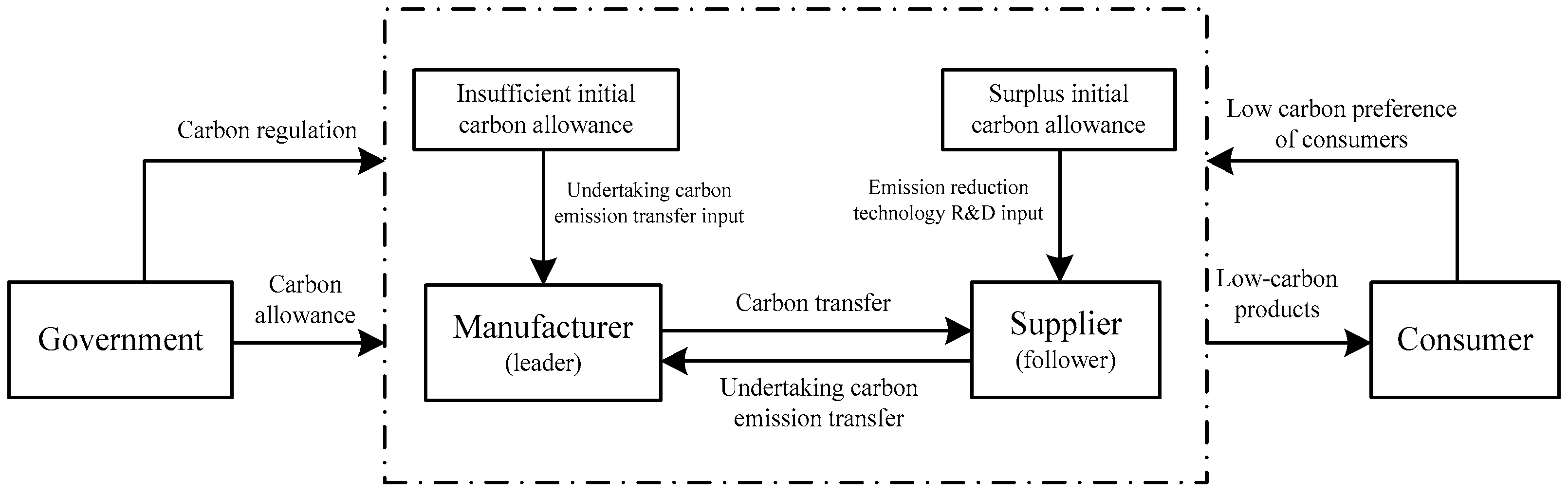
This paper considers a supply chain that consists of a single manufacturer and a single supplier. The former’s initial carbon quota is insufficient, whereas the latter’s initial carbon quota has a surplus. To maximize profit, the manufacturer uses its dominant position in the supply chain to transfer a portion of its carbon emissions that are difficult to reduce to the supplier. The supplier will fully receive carbon emission transfers from the manufacturer, as shown in Figure 1.
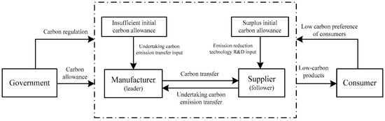
Figure 1.
Manufacturer-supplier carbon emission transfer process.
This paper compares the profit before and after the transfer of carbon emissions in the supply chain and distinguishes the rational and irrational transfer of carbon emissions in the supply chain from the perspective of the supply chain. If the profit of each member of the supply chain and the overall profit of the supply chain increases after the carbon emission transfer among supply chain enterprises, it indicates that the transfer is a rational transfer of carbon emissions in the supply chain. On the contrary, if there is a profit reduction for any member in the supply chain, the transfer is an irrational transfer of carbon emissions in the supply chain. Therefore, after a transfer, one of the three scenarios shown in Table 1 will be obtained.

Table 1.
Scenario analysis of carbon emission transfers in supply chains.
According to the above criteria for the irrational transfer of carbon emissions in the supply chain:
- (1)
- Scenario 1 is the rational transfer of supply chain carbon emissions. The transfer increases the profits of the manufacturer, supplier, and the entire supply chain.
- (2)
- Scenario 2 is the irrational transfer of supply chain carbon emissions. The profits of the manufacturer and the entire supply chain increase, but that of the supplier decreases after the transfer.
- (3)
- Scenario 3 also represents the irrational transfer of supply chain carbon emissions. Only the manufacturer’s profit increases, whereas those of the other two entities decrease.
This paper analyzes the irrational transfer of supply chain carbon emissions in Scenario 2 and Scenario 3.
2.2. Assumptions of the Model
This study constructed a Steinberg game model of the carbon emission transfers of a major manufacturer and their upstream suppliers. For the model, the following hypotheses were formulated:
- (1)
- Both the supplier and the manufacturer are rational decision-makers of risk neutrality, the information is completely symmetrical, and the manufacturer consumes one unit of raw material provided by the supplier for each unit of production.
- (2)
- Consumers prefer low-carbon products and suppliers can reduce emissions at a positive rate to promote the prices of low-carbon products [54,55,56]. In addition, the transfers of carbon emissions from suppliers to manufacturers is reflected in the reduction in carbon emissions per unit of the supplier’s product. Therefore, the market price of a low-carbon product is set to , where is the retail price when no factors are taken into account, represents the price of the demand-sensitive factor, and represents the intensity of the consumers’ low-carbon awareness. Qi, Wang and Bai, and Panda et al. have formulated similar hypotheses [57,58].
- (3)
- The supplier and manufacturer’s unit production costs are expressed as and , respectively. To ensure that the supply chain is profitable, .
- (4)
- According to Zhang, Wang and You, Zhou and Ye, and Yu et al., suppliers need to invest in the research and development (R&D) of emission reduction technologies [59,60,61]. Our study assumed that the R&D costs are , where indicates the investment level coefficient for emission reduction. The difficulty of reducing emissions increases with the number of emissions to be reduced. The required input increases sharply.
- (5)
- It is assumed that the processing cost after the supplier undertakes the carbon emission transfer is , where represents the cost coefficient after the supplier undertakes the carbon emission transfer, which mainly reflects the cost invested by suppliers to offset the transfer of carbon emissions from manufacturers. For example, companies such as Apple and Dell have transferred part of their carbon emissions to their suppliers in the process of manufacturing outsourcing. Suppliers need to use manpower, material resources, emission reduction technology, and other means to offset and deal with these carbon emissions. Therefore, suppliers need to invest funds to undertake the transfer of carbon emissions.
Symbolic descriptions of the parameters and variables are given in Table 2.
Table 2.
Symbolic descriptions of parameters and variables.
3. Identification of Irrational Transfers
From a comparative analysis of the changes in the profits of the manufacturers, suppliers and supply chains in two scenarios, one with and the other without transfers, the identification intervals of irrational transfers were extracted and the influence of each coefficient on the recognition interval was analyzed.
3.1. Ignoring Carbon Emission Transfers
The manufacturer plays the Steinberg game with the upstream supplier as the leader. The supplier’s and manufacturer’s respective profit functions are:
The manufacturer’s margin per unit is . The profit functions can be further expressed as:
The reverse induction method is used to obtain the optimal decisions of the manufacturer and supplier. (N signifies that the transfers have been ignored.)
When :
The profits are obtained by:
3.2. Acknowledging Carbon Emission Transfers
When there is a transfer , the profit functions are:
The optimal decisions of the manufacturer and supplier are as follows. (T signifies that the transfer has been acknowledged.)
When :
The profits are obtained by:
3.3. Identification Interval of Irrational Transfers
Table 1 implies that irrational transfers under Scenario 2 must meet the following conditions:
To identify the irrational transfer of supply chain carbon emissions under Scenario 3, the following conditions must be met:
The solutions to the above inequations require the value range of , i.e., the irrational interval of supply chain carbon emission transfer under Scenario 2 and Scenario 3. Thus, Conclusion 1 and Conclusion 2 can be formulated. The proofs of Conclusion 1 and 2 is given in the Appendix A.
Conclusion 1.
When , the irrational transfer interval under Scenario 2 is ; when , it is [].
Conclusion 1 shows that within the irrational transfer range of supply chain carbon emissions shown in Scenario 2, the manufacturer and supply chain increases in their profits, and the supplier’s profit decreases. After the manufacturer has transferred a portion of the emissions, the increase in the product’s market demand improves the supplier’s sales profit. However, the supplier’s investment in emission reduction research and development or received carbon emission transfer is too large, leading to a situation in which the supplier’s income situation still cannot be improved. However, the increase in the supply chain’s overall profit suggests room for improvement. Manufacturers can optimize and regulate irrational carbon emission transfers to encourage the initiation of rational carbon emission transfers.
Conclusion 2.
When , the irrational transfer interval under Scenario 3 is [].
Conclusion 2 shows that in the irrational transfer range of supply chain carbon emissions shown in Scenario 3, although the manufacturer’s profit increases, the supplier’s and the supply chain’s overall profit decrease. This shows that the transfer of carbon emissions has damaged the interests of other members of the supply chain and cannot make up for it. Supply chain members cannot increase the profits of supply chain members through profit redistribution and other methods. Suppliers realize that they accept the carbon emission transfer in this context, and even if they cooperate with the manufacturer, they will not be able to improve their own profitability, and will not accept the carbon emission transfer of the manufacturer. At this time, if the supplier is to actively accept the carbon emission transfer of the manufacturer, the government needs to intervene appropriately, increase the carbon emission quota to the manufacturer, or provide monetary subsidies so that the overall profit of the supply chain after the carbon emission transfer is not lower than the transfer. They may also impose penalties on companies that transfer carbon emissions, or even compulsorily close these companies.
Corollary 1.
When , the irrational transfer range of carbon emissions [] under Scenario 2 exists, but the irrational transfer range of carbon emissions under Scenario 3 does not exist.
Corollary 2.
When , there are both the irrational transfer interval of carbon emissions under Scenario 2 [] and the irrational transfer interval of carbon emissions under Scenario 3 [].
Corollaries 1 and 2 can be combined to obtain Conclusion 3.
Conclusion 3.
When , the irrational transfer range of carbon emissions in the supply chain is [].
The irrational transfer interval’s range is not static but changes with the supplier’s capacity coefficient to receive transfers and the related investment level coefficient, the investment level coefficient of reduction, and the intensity of the consumers’ low-carbon awareness. Corollaries 3 and 4 state how these coefficients affect the irrational transfer interval’s range. The proofs of Corollaries 3 and 4 is given in the Appendix A.
Corollary 3.
The supply chain carbon emission irrational transfer interval [] increases with the supplier’s capacity coefficient .
Corollary 3 shows that when the supplier’s ability to undertake carbon emissions transfer is greater, the supplier actually accepts more carbon emissions transfer. This is because the suppliers are restricted by the company’s production capacity or emission reduction technology, and cannot well detract from the manufacturer’s carbon emission transfer. At this time, if the supplier undertakes too much carbon emission transfer, the cost of undertaking carbon transfer will increase. In order to reduce the cost of undertaking carbon emission transfers, suppliers will reduce the amount of carbon emissions transferred. Therefore, as far as the supplier is concerned, as the supplier’s ability to undertake carbon emission transfer increases, the amount of carbon emissions transferred to increase its profits continues to decrease, and the range of carbon emission transfers that reduce its profits continues to increase; that is, carbon emissions increase. The range of the irrational transfer interval keeps increasing.
Corollary 4.
The supply chain carbon emission irrational transfer interval [] increases with the investment level coefficient for receiving transfers, the investment level coefficient of emission reduction , and the consumers’ low-carbon awareness intensity .
Corollary 4 shows the following to be the case: (1) When the investment cost coefficient of undertaking carbon emission transfer is larger, the cost for the supplier to undertake the unit product carbon emission transfer is higher. Accepting excessive carbon emission transfer from the manufacturer will directly cause it to undertake the carbon transfer. In order to reduce the cost of undertaking carbon emission transfer, suppliers will reduce the amount of carbon emission transfer. (2) In the same way, an increase in the emission reduction investment cost coefficient will result in a substantial increase in the supplier’s emission reduction cost, and the supplier will also reduce the amount of carbon emission transfer in order to reduce the cost. As a result, the price of the product drops, which in turn leads to lower supplier profits. Therefore, for suppliers, as these coefficients increase, the amount of carbon emissions transferred to increase their profits will continue to decrease, and the range of carbon emissions transferred to reduce their profits will continue to increase. That is, the range of the irrational shift of carbon emissions continues to increase. (3) The higher the intensity of the consumers’ low-carbon awareness, the higher are their requirements for low-carbon products. However, the manufacturers’ transfers would actually increase the suppliers’ burden for reduction and lead to a decrease in their emissions per unit product. Therefore, when consumers prefer more low-carbon products, manufacturers will transfer fewer emissions per unit product.
4. Optimization of Irrational Transfers
Under the current situation of increasingly standardized carbon regulation environment, carbon emission transfer, as a means of regulating carbon emission resources among enterprises in the supply chain, also needs to be reasonably guided and regulated to prevent the formation of irrational transfer and avoid the overall problems of enterprises and the supply chain. Irrational transfer and loss of benefits. Therefore, it is particularly important to optimize the irrational transfer of carbon emissions.
It can be seen from Section 3 that in the irrational transfer range of supply chain carbon emissions shown in Scenario 3, only the manufacturer’s profit increases, while the supplier’s and the supply chain’s overall profit decrease. The coordination of resources within the supply chain optimizes the irrational transfer. Therefore, this section only optimizes the irrational transfer of carbon emissions in the supply chain under Scenario 2.
In the irrational transfer range of supply chain carbon emissions shown in Scenario 2, the overall profits of manufacturers and the supply chain have increased, but the profits of suppliers have decreased. This shows that in this irrational transfer interval, there is room for optimizing the irrational transfer of carbon emissions in the supply chain by rationally designing contracts to coordinate the relationship between manufacturers and suppliers in the supply chain. At this time, in order to ensure that their profits will not decrease, the supplier will require the manufacturer to give himself some compensation. In order to alleviate the pressure of carbon emission reduction, the initiator and manufacturer of carbon emission transfer have the incentive to design an optimized strategy for the irrational transfer of carbon emissions in the supply chain. The strategy must have the following characteristics: Compared with the case of carbon-free transfer, it is ensured that the optimized profits of manufacturers, suppliers and the overall supply chain are not lower than the profit of the carbon-free transfer; that is, the rational transfer of supply chain carbon emissions is achieved. Therefore, when , the manufacturer can bear of the costs while the supplier bears the remainder (1 − . Therefore, this arrangement will lead to a cost-sharing contract to optimize irrational transfers under Scenario 2.
4.1. Interval Optimization of Irrational Transfers
When , irrational transfers occur. The manufacturer will bear , i.e., , of the costs. The manufacturer and retailer will implement a contract , where are obtained by Equations (12)–(14). This contract is designed to ensure that the profits of both parties increase. The superscript T in Equations (12)–(14) has been changed to D to represent the corresponding variables with a contract. The corresponding formulas are obtained:
To ensure the validity of the contract, the profits of the manufacturers and suppliers should not be less than those gained in the absence of transfers, i.e., satisfies the following inequations:
The solution to the above set of inequations permits the scoring of the value range of the share rate .
Conclusion 4.
When the manufacturer’s share rate satisfies , then the manufacturer-led contract can encourage the shift of transfers from irrational to rational:
The proofs of Conclusion 4 is given in the Appendix A.
When the manufacturer’s unit product carbon emission transfer amount is , as long as the manufacturer’s cost sharing rate for the supplier’s carbon emission transfer meets , compared with the scenario of no carbon emission transfer, the profits of both manufacturers and suppliers have increased, and the overall profits of the supply chain have increased. Therefore, the carbon emission transfer cost sharing contract led by the manufacturer can realize the transformation of supply chain carbon emission transfer from irrational to rational.
4.2. Point Optimization of Irrational Transfers
As mentioned in Section 4.1, a continuous transfer cost-share rate can optimize irrational transfers. However, to give a value range from which suppliers can choose is impossible in practice. Therefore, to ensure that the agreement between the manufacturer and supplier is fair and reasonable, a Nash bargaining model was used to determine the cost-share rate.
Suppose that the bargaining power of the manufacturer is and the bargaining power of the supplier is . The bargaining power here may include the economic and psychological characteristics, such as brand value or negotiation skills, of supply chain companies [62]. Let , which represents the relative bargaining power of the manufacturer, and , which represents that of the supplier. The point of conflict in the bargaining is , which means that when no agreement is reached, everyone accepts the original agreement, i.e., they proceed without a contract. The feasible domain of bargaining is:
where and have already been expressed by Equations (22) and (23), respectively. In the bargaining process, both the manufacturer and supplier want their and to be as large as possible. The Nash bargaining solution is the maximum value of the Nash product in the feasible range for bargaining [63]. The following formula expresses the Nash bargaining model for this problem:
Solving this problem gives:
Substituting and into Equations (28) and (29), we obtain:
Combining the last two equations, we obtain:
Let , which represents the relative bargaining power of the manufacturer, then , which represents the relative bargaining power of the supplier. We obtain: . The respective profits of the manufacturer and supplier are:
From the above descriptions, Conclusion 5 can be drawn.
Conclusion 5.
The bargaining power of the manufacturer to determine the share rate in the transfer cost-sharing contract is and the bargaining power of the supplier is , so: (1) the cost-share rate determined by the Nash bargaining model is given by Equation (33); (2) under a contract led by the manufacturer, the profits of both parties are given by Equations (34) and (35), respectively.
By adjusting the value of α, the share rate can be changed in the rational range, the free distribution of residual profits can be realized, and the irrational transfer can be optimized. The bargaining powers of the manufacturer and supplier directly affect how much profit they can earn. When the manufacturer’s core competitiveness and bargaining power are stronger, they will share in less of the supplier’s transfer costs, then the profit of the former will increase, whereas that of the latter will decrease.
So far, an optimization strategy for irrational carbon emission transfers in the supply chain has been found, i.e., a supply chain carbon emission transfer cost-sharing contract has been designed according to , , and Equation (33). Thus, the transformation from an irrational to a rational transfer is realized.
5. Numerical Analysis
To further verify the validity of the above conclusions, numerical calculations were conducted. According to data released by the World Bank in 2019 [64], the carbon price parameter . Considering that the front end of the supply chain is generally high-carbon emission enterprises, the initial carbon emissions of manufacturers and suppliers are set as and . In actual production and operation, the government will allocate the initial carbon allowance to the company based on the company’s total historical carbon emissions. Combined with related literature [65], set the manufacturer’s initial carbon allowance , and the supplier’s initial carbon allowance . In accordance with our hypotheses and those of related studies [66], the following basic parameters were set: , , , , , , and .
In the absence of carbon emission transfers, the supplier’s optimal emission reduction is , and the wholesale price gives the optimal profit . The manufacturer decides the best product. The order quantity is and the optimal profit is obtained. The total profit of the supply chain is .
5.1. Interval Identification of Irrational Transfers
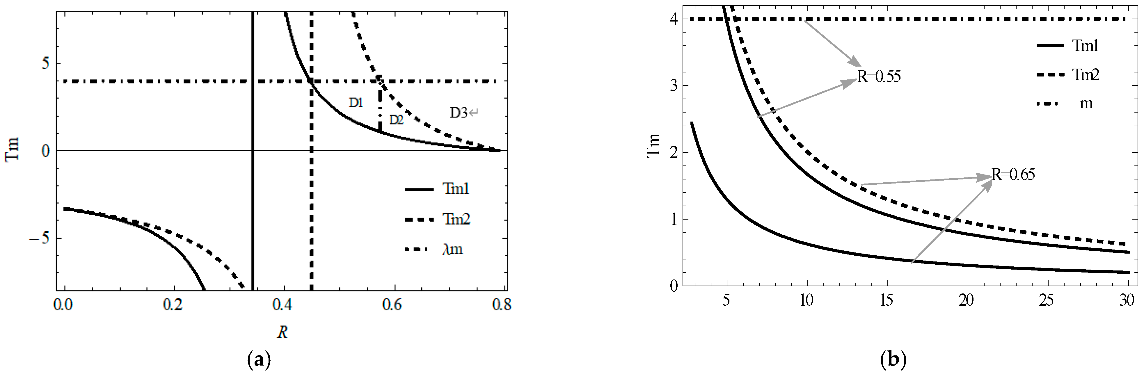
Figure 2a compares the manufacturer’s profits before and after a transfer. When , the latter profit is higher. Secondly, it analyzes the changes in the overall profits of suppliers and the supply chain before and after carbon emission transfer when . Figure 2b,c show that it is found that when , the irrational transfer range of supply chain carbon emissions under Scenario 2 is (. When , the supply chain carbon emission irrational transfer interval under Scenario 2 is (, and the irrational transfer range of supply chain carbon emissions under Scenario 3 is (.
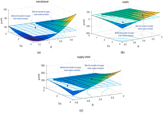
Figure 2.
(a) Manufacture’s profit before and after a transfer. (b) Supply’s profit before and after a transfer. (c) Supply chain’s profit before and after a transfer.
To verify Conclusion 1 further, the supplier’s capacity coefficient R to receive transfers is fixed. Figure 3a,b show the situation when and , respectively. Specifically: (1) as increases, the overall profit of the supplier and supply chain first increases but then decreases; (2) when , the irrational transfer interval under Scenario 2 is [0.52, 1.64]. The irrational transfer interval under Scenario 3 is . (3) When , the irrational transfer interval under Scenario 2 is [1.36, 4].
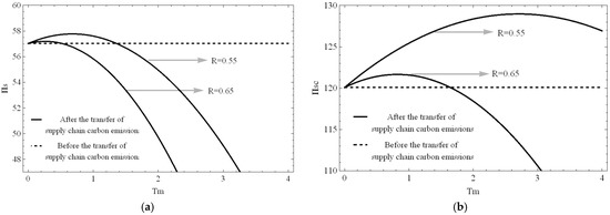
Figure 3.
(a) Supply’s profit before and after a transfer. (b) Supply chain’s profit before and after a transfer.
5.2. Influence Variables Analysis of Irrational Transfer Intervals
Figure 4a reflects the influence of the supplier’s ability to undertake carbon emission transfer on the irrational interval of carbon emission transfer in the supply chain. For the D3 area, that is, when , the figure enclosed by and . At this time, [] is the irrational transfer range under Scenario 3. This range will decrease as the supplier’s ability to undertake carbon emissions transfer increases. For the D1 area, namely , at this time , the supply chain carbon emission irrational transfer interval under Scenario 2 is []; affected by the upper limit, this interval will increase with the decreasing of . For the D2 area, namely , , the supply chain carbon emission irrational transfer interval under Scenario 2 is [], and the interval increases as decreases.
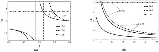
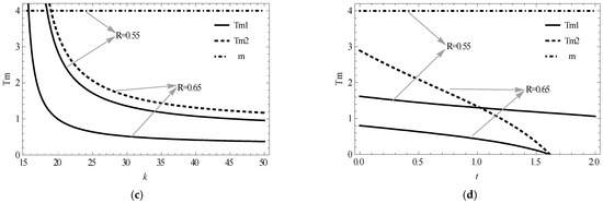
Figure 4.
(a) Influences of on irrational transfer interval. (b) Influences of on irrational transfer interval. (c) Influences of on irrational transfer interval. (d) Influences of on irrational transfer interval.
To eliminate the influence of on the other parameters, is set to 0.55 and 0.65. Figure 4b–d show that both and decrease as , , and increase. When and as the values of , , and decrease, so does the irrational transfer interval under Scenario 2 []. When and as the values of , , and decrease, the irrational transfer interval under Scenario 2 [] increases. However, the supply chain carbon emission irrational transfer interval under Scenario 3 [] will be smaller.
5.3. Optimization of Irrational Transfers
As mentioned in Section 5.1, when , the irrational transfer interval’s range is [0.52, 1.64]. When , the irrational transfer interval’s range is [1.36, 4]. For convenience, we verify Conclusions 4 and 5. When , , and when , .
First, we verify the effectiveness of interval optimization. When and , can be obtained. When and , can be obtained to verify Conclusion 4.
Second, we verify the effectiveness of point optimization and compare the incomes of the supply chain’s members with different relative bargaining powers. Table 3 shows the influence of on income distribution.
Table 3.
Incomes of supply chain members under different relative bargaining powers.
Table 3 shows that: (1) the stronger the relative bargaining power of the manufacturer, the lower are the share rates of the cost of the transfer received by the supplier and the cost shared by the manufacturer; (2) in the absence of a transfer, the manufacturer’s profit is 63.05, the supplier’s profit is 57.03, and the supply chain’s overall profit is 120.08, all of which are less than the profit obtained under a transfer cost-sharing contract. Hence, such a contract based on the bargaining model is an effective strategy for optimizing irrational transfers, and can realize the transformation to rational transfers.
6. Main Conclusions and Practical Implications
6.1. Main Conclusions
This study examined the implications of irrational transfers of carbon emission. A model of a Steinberg game was constructed to study the identification of irrational transfers of carbon emission led by manufacturers. Then, a supply chain carbon emission transfer cost-sharing contract with a bargaining model was designed to optimize the irrational transfers. The main conclusions of this study are as follows.
(1) When the supplier’s carbon emission transfer capacity coefficient is small, there is an irrational carbon emission transfer interval under Scenario 2, but there is no carbon emission irrational transfer interval under Scenario 3; when the supplier’s carbon emission transfer capacity coefficient is large, there is both an irrational transfer interval of carbon emissions in Scenario 2 and an irrational transfer interval of carbon emissions in Scenario 3.
(2) The scope of the supply chain carbon emission irrational interval is affected by the supplier’s ability to undertake carbon emission transfer. When the supplier’s carbon emission transfer capacity coefficient is small, the irrational range of the supply chain carbon emission transfer is larger and increases with the increasing of the coefficient; when the supplier’s carbon emission transfer capacity coefficient is large, the irrational range of the supply chain’s carbon emission transfer is relatively small and decreases with the increasing of the coefficient.
(3) When the supplier’s carbon emission transfer capacity coefficient is small, the increase in the supplier’s carbon emission transfer investment cost coefficient and emission reduction investment cost coefficient will cause the irrational transfer range of carbon emissions in the supply chain to gradually increase. Therefore, suppliers need to pay attention to their own investment costs for undertaking carbon emissions transfer as well as their emission reduction investment costs. When these two costs are high, the scope of the irrational range of carbon emission transfer in the supply chain will expand, and the transfer of carbon emissions will cause the loss of suppliers’ own profits.
(4) When the supplier’s ability to undertake carbon emissions transfer has a small coefficient, the range of irrational transfer of carbon emissions in the supply chain is directly proportional to the intensity of consumers’ low-carbon awareness. Therefore, when exploring the impact of irrational transfer of carbon emissions on the supply chain, it is necessary to consider the impact of consumers’ low-carbon awareness on the transfer of carbon emissions. The stronger the consumers’ low-carbon awareness and the more sensitive they are to low-carbon products, the greater the probability of irrational transfer of carbon emissions.
(5) When the manufacturer’s share of the supplier’s cost of transfers meets certain conditions, the supply chain’s members can optimize irrational transfers by establishing transfer cost-sharing contracts, for which a Nash bargaining model can be used to determine the value of the share rate.
6.2. Practical Implications
The practical implications of this study are mainly reflected in three aspects: one is the inspiration to the initiator of the carbon emission transfer in the supply chain; the second is the inspiration to the undertaker of the carbon emission transfer in the supply chain; and the third is the inspiration to the policy makers.
(1) For the initiators of carbon emission transfer in the supply chain, first, they can choose companies with strong carbon emission transfer capabilities to give priority to cooperation in order to, on the one hand, expand the rational range of carbon emission transfer in the supply chain, and reduce obstacles to cooperation between the two parties; on the other hand, they can reduce or even eliminate the irrational range of carbon emission transfer in the supply chain, and reduce the possibility of the transfer party being pressured by the government’s compulsory policy. Secondly, it is necessary to continue to pay attention to consumers’ low-carbon awareness, analyze consumers’ low-carbon purchase behavior preferences, and communicate feedback with the carbon transfer undertaker in a timely manner to reduce the profit loss caused by the carbon emission transfer to the undertaker and to reduce irrational transfer.
(2) For the undertaker of supply chain carbon emissions transfer, first of all, efforts to improve its ability to receive carbon emissions transfer can help them obtain long-term cooperation opportunities with the transferer, thereby gaining more benefits and improving their own and the overall supply chain’s efficiency and sustainability. Secondly, it is also necessary to reasonably control the investment cost of undertaking carbon emission transfer and emission reduction investment cost. Only by balancing the relationship between emission reduction investment and undertaking carbon transfer investment can the negative impact of irrational transfer on its own profits be reduced.
In short, if both parties in the supply chain want to implement carbon emission transfer more reasonably and reduce the adverse impact of irrational transfer on the supply chain, they need to fully utilize and integrate the carbon allowance resources within the supply chain, and cooperate to maximize the use of carbon allowance resources. In so doing, they can better respond to changes and risks in a carbon regulatory environment and enhance the stability and continuity of the supply chain.
(3) As the issuer and monitor of carbon regulatory policies, the government should pay attention to the irrational transfer phenomenon within the supply chain, and can formulate different policies for the different levels of carbon emission transfers of different companies. For companies with low carbon emissions transfer, under the guidance of market rules, a rational transfer of carbon emissions can be formed spontaneously without excessive government intervention. For companies with excessively high carbon emissions transfer, the market will tend towards “failure” in these cases. The government can appropriately increase the carbon allowances of the transfer initiators to ease excessive carbon regulatory pressure, or force them to implement emission reductions or even close them through tough policies. As for companies whose carbon emission transfer level is between the two, the government can also hand it over to the market. Therefore, as far as the government is concerned, it only needs to pay attention to companies that transfer excessively high carbon emissions, and leave other companies to the market.
6.3. Research Limitations and Future Work
There are still some limitations in this study, which need to be further explored and improved. (1) Scenario 3 shows the unregulated irrational transfer of carbon emissions in the supply chain. In the future, the government can be included in the supply chain system to study the optimization strategy for the irrational transfer of supply chain carbon emissions under this scenario based on the government’s dynamic quota. (2) This article considers the problem of identifying and optimizing the irrational transfer of carbon emissions between supply chain companies under complete information. If there is information asymmetry between supply chain companies, how will the irrational transfer of carbon emissions in the supply chain be identified and optimized? (3) This article only defines the irrational transfer of carbon emissions in the supply chain from a single dimension of corporate profits. If environmental dimensions such as carbon emissions are included in the identification criteria, the identification and optimization of irrational transfers of carbon emissions in the supply chain will be more important, complex and difficult. Therefore, the research will be further enriched and perfected from these three aspects in the future.
Author Contributions
Conceptualization, L.S.; methodology, L.S.; software, S.F.; validation, L.S. and S.F.; formal analysis, S.F.; investigation, L.S.; resources, L.S.; data curation, S.F.; writing—original draft preparation, S.F.; writing—review and editing, L.S.; visualization, S.F.; supervision, L.S.; project administration, L.S.; funding acquisition, L.S. All authors have read and agreed to the published version of the manuscript.
Funding
This study was supported by the National Natural Science Foundation of China (Nos.71874071 and 71473107), and the Ministry of Education in China Youth Fund Project of Humanities and Social Sciences (No.16YJCZH153).
Institutional Review Board Statement
Not applicable.
Informed Consent Statement
Not applicable
Data Availability Statement
The selection of carbon price parameters is determined according to the State and Trends of Carbon Pricing 2019 issued by the World Bank in 2019. This data can be found here: http://hdl.handle.net/10986/31755 (accessed on 1 January 2022).
Conflicts of Interest
The authors declare no conflict of interest.
Appendix A
Proof of Conclusion 1.
(1) When ,
is obtained.
(2) From ,
When , then .
(3) From ,
When , then .
Among this,
In addition, because ,. In summary, when , .
Furthermore, considering , from , when , then .
Among this,
Therefore, when , ; when , . □
Proof of Conclusion 2.
(1) When ,
is obtained.
(2) From ,
When , then .
(3) From ,
When , then .
In addition, because , is obtained. Furthermore, when , then .
Therefore, when , . □
Proof of Corollary 3–4.
Find the partial derivatives of with respect to , , , and to obtain:
(1) When , .
(2) When , .
(3) When , .
(4) When , . □
Proof of Conclusion 4.
Under the carbon transfer cost sharing contract, the profit functions of manufacturers and suppliers are:
In order to achieve the coordination of the supply chain, the profits of the manufacturers and suppliers at this time should be at least not less than the situation when carbon emission transfer is not considered; that is, γ satisfies the following inequality group:
Solving the above set of inequalities, the score burden γ satisfies the interval in Conclusion 4. □
References
- Guertler, B.; Spinier, S. When does operational risk cause supply chain enterprises to tip? A simulation of intra-organizational dynamics. Omega 2015, 57, 54–69. [Google Scholar] [CrossRef]
- Silva, M.E.; Figueiredo, M.D. Practicing sustainability for responsible business in supply chains. J. Clean. Prod. 2020, 251, 119621. [Google Scholar] [CrossRef]
- Cao, E.; Du, L.; Ruan, J. Financing preferences and performance for an emission-dependent supply chain: Supplier vs. Bank. Int. J. Prod. Econ. 2019, 208, 383–399. [Google Scholar] [CrossRef]
- Wang, L.; Hui, M. Research on joint emission reduction in supply chain based on carbon footprint of the product. J. Clean. Prod. 2020, 263, 121086. [Google Scholar] [CrossRef]
- Mokhtar, A.R.M.; Genovese, A.; Brint, A.; Kumar, N. Supply chain leadership: A systematic literature review and a research agenda. Int. J. Prod. Econ. 2019, 216, 255–273. [Google Scholar] [CrossRef]
- Zhang, S.; Wang, C.; Yu, C.; Ren, Y. Governmental cap regulation and manufacturer’s low carbon strategy in a supply chain with different power structures. Comput. Ind. Eng. 2019, 134, 27–36. [Google Scholar] [CrossRef]
- Wang, F.; Sun, J.; Liu, Y.S. Institutional pressure, ultimate ownership, and corporate carbon reduction engagement: Evidence from china. J. Bus. Res. 2019, 104, 14–26. [Google Scholar] [CrossRef]
- Sun, L.; Cao, X.; Alharthi, M.; Zhang, J.; Taghizadeh-Hesary, F.; Mohsin, M. Carbon emission transfer strategies in supply chain with lag time of emission reduction technologies and low-carbon preference of consumers. J. Clean. Prod. 2020, 264, 121664. [Google Scholar] [CrossRef]
- Bai, Q.; Gong, Y.; Jin, M.; Xu, X. Effects of carbon emission reduction on supply chain coordination with vendor-managed deteriorating product inventory. Int. J. Prod. Econ. 2019, 208, 83–99. [Google Scholar] [CrossRef]
- Duan, C.; Chen, B.; Feng, K.; Liu, Z.; Hayat, T.; Alsaedi, A.; Ahmad, B. Interregional carbon flows of china. Appl. Energy 2018, 227, 342–352. [Google Scholar] [CrossRef]
- Wang, Q.; Liu, Y.; Wang, H. Determinants of net carbon emissions embodied in sino-german trade. J. Clean. Prod. 2019, 235, 1216–1231. [Google Scholar] [CrossRef]
- Shi, J.; Li, H.; An, H.; Guan, J.; Arif, A. Tracing carbon emissions embodied in 2012 chinese supply chains. J. Clean. Prod. 2019, 226, 28–36. [Google Scholar] [CrossRef]
- Wang, W.; Hu, Y. The measurement and influencing factors of carbon transfers embodied in inter-provincial trade in china. J. Clean. Prod. 2020, 270, 122460. [Google Scholar] [CrossRef]
- Wang, S.; Wang, X.; Tang, Y. Drivers of carbon emission transfer in china—An analysis of international trade from 2004 to 2011. Sci. Total Environ. 2020, 709, 135924. [Google Scholar] [CrossRef]
- Wang, M.; Li, Y.; Li, M.; Shi, W.; Quan, S. Will carbon tax affect the strategy and performance of low-carbon technology sharing between enterprises? J. Clean. Prod. 2019, 210, 724–737. [Google Scholar] [CrossRef]
- Shi, Y.; Han, B.; Zeng, Y. Simulating policy interventions in the interfirm diffusion of low-carbon technologies: An agent-based evolutionary game model. J. Clean. Prod. 2020, 250, 119449. [Google Scholar] [CrossRef]
- Ghalehkhondabi, I.; Maihami, R.; Ahmadi, E. Optimal pricing and environmental improvement for a hazardous waste disposal supply chain with emission penalties. Util. Policy 2020, 62, 101001. [Google Scholar] [CrossRef]
- Peng, H.; Pang, T.; Cong, J. Coordination contracts for a supply chain with yield uncertainty and low-carbon preference. J. Clean. Prod. 2018, 205, 291–302. [Google Scholar] [CrossRef]
- Yuyin, Y.; Jinxi, L. The effect of governmental policies of carbon taxes and energy-saving subsidies on enterprise decisions in a two-echelon supply chain. J. Clean. Prod. 2018, 181, 675–691. [Google Scholar] [CrossRef]
- Waltho, C.; Elhedhli, S.; Gzara, F. Green supply chain network design: A review focused on policy adoption and emission quantification. Int. J. Prod. Econ. 2019, 208, 305–318. [Google Scholar] [CrossRef]
- Li, J.; Wang, L.; Tan, X. Sustainable design and optimization of coal supply chain network under different carbon emission policies. J. Clean. Prod. 2020, 250, 119548. [Google Scholar] [CrossRef]
- Bian, J.; Zhao, X. Tax or subsidy? An analysis of environmental policies in supply chains with retail competition. Eur. J. Oper. Res. 2020, 283, 901–914. [Google Scholar] [CrossRef]
- Kaur, H.; Singh, S.P. Modeling low carbon procurement and logistics in supply chain: A key towards sustainable production. Sustain. Prod. Consum. 2017, 11, 5–17. [Google Scholar] [CrossRef]
- Wang, J.; Wan, Q.; Yu, M. Green supply chain network design considering chain-to-chain competition on price and carbon emission. Comput. Ind. Eng. 2020, 145, 106503. [Google Scholar] [CrossRef]
- Zu, Y.; Chen, L.; Fan, Y. Research on low-carbon strategies in supply chain with environmental regulations based on differential game. J. Clean. Prod. 2018, 177, 527–546. [Google Scholar] [CrossRef]
- Sherafati, M.; Bashiri, M.; Tavakkoli-Moghaddam, R.; Pishvaee, M.S. Supply chain network design considering sustainable development paradigm: A case study in cable industry. J. Clean. Prod. 2019, 234, 366–380. [Google Scholar] [CrossRef]
- Valderrama, C.V.; Santibanez-González, E.; Pimentel, B.; Candia-Véjar, A.; Canales-Bustos, L. Designing an environmental supply chain network in the mining industry to reduce carbon emissions. J. Clean. Prod. 2020, 254, 119688. [Google Scholar] [CrossRef]
- Sterman, J.D.; Dogan, G. “I’m not hoarding, I’m just stocking up before the hoarders get here”: Behavioral causes of phantom ordering in supply chains. J. Oper. Manag. 2015, 39, 6–22. [Google Scholar] [CrossRef]
- Zaid, A.A.; Jaaron, A.A.M.; Talib Bon, A. The impact of green human resource management and green supply chain management practices on sustainable performance: An empirical study. J. Clean. Prod. 2018, 204, 965–979. [Google Scholar] [CrossRef]
- Kumar, A.; Moktadir, M.A.; Khan, S.A.R.; Garza-Reyes, J.A.; Tyagi, M.; Kazançoğlu, Y. Behavioral factors on the adoption of sustainable supply chain practices. Resour. Conserv. Recycl. 2020, 158, 104818. [Google Scholar] [CrossRef]
- Bendoly, E.; Croson, R.; Goncalves, P.; Schultz, K. Bodies of knowledge for research in behavioral operations. Prod. Oper. Manag. 2010, 19, 434–452. [Google Scholar] [CrossRef]
- Yang, L.; Hao, C.; Yang, X. Pricing and carbon emission reduction decisions considering fairness concern in the big data era. Procedia CIRP 2019, 83, 743–747. [Google Scholar] [CrossRef]
- Chan, C.K.; Zhou, Y.; Wong, K.H. An equilibrium model of the supply chain network under multi-attribute behaviors analysis. Eur. J. Oper. Res. 2018, 275, 514–535. [Google Scholar] [CrossRef]
- Wang, Y.; Fan, R.; Shen, L.; Miller, W. Recycling decisions of low-carbon e-commerce closed-loop supply chain under government subsidy mechanism and altruistic preference. J. Clean. Prod. 2020, 259, 120883. [Google Scholar] [CrossRef]
- Zhou, M.; Govindan, K.; Xie, X. How fairness perceptions, embeddedness, and knowledge sharing drive green innovation in sustainable supply chains: An equity theory and network perspective to achieve sustainable development goals. J. Clean. Prod. 2020, 260, 120950. [Google Scholar] [CrossRef]
- Wang, Y.; Yu, Z.; Jin, M.; Mao, J. Decisions and coordination of retailer-led low-carbon supply chain under altruistic preference. Eur. J. Oper. Res. 2021, 293, 910–925. [Google Scholar] [CrossRef]
- Fan, R.; Lin, J.; Zhu, K. Study of game models and the complex dynamics of a low-carbon supply chain with an altruistic retailer under consumers’ low-carbon preference. Phys. A Stat. Mech. Appl. 2019, 528, 121460. [Google Scholar] [CrossRef]
- Zhang, L.; Zhou, H.; Liu, Y.; Lu, R. Optimal environmental quality and price with consumer environmental awareness and retailer’s fairness concerns in supply chain. J. Clean. Prod. 2019, 213, 1063–1079. [Google Scholar] [CrossRef]
- Li, Q.; Xiao, T.; Qiu, Y. Price and carbon emission reduction decisions and revenue-sharing contract considering fairness concerns. J. Clean. Prod. 2018, 190, 303–314. [Google Scholar] [CrossRef]
- Qin, Q.; Jiang, M.; Xie, J.; He, Y. Game analysis of environmental cost allocation in green supply chain under fairness preference. Energy Rep. 2021, 7, 6014–6022. [Google Scholar] [CrossRef]
- Zhao, S.; Zhu, Q. A risk-averse marketing strategy and its effect on coordination activities in a remanufacturing supply chain under market fluctuation. J. Clean. Prod. 2018, 171, 1290–1299. [Google Scholar] [CrossRef]
- Lu, X.; Shang, J.; Wu, S.-Y.; Hegde, G.G.; Vargas, L.; Zhao, D. Impacts of supplier hubris on inventory decisions and green manufacturing endeavors. Eur. J. Oper. Res. 2015, 245, 121–132. [Google Scholar] [CrossRef]
- He, R.; Xiong, Y.; Lin, Z. Carbon emissions in a dual channel closed loop supply chain: The impact of consumer free riding behavior. J. Clean. Prod. 2016, 134, 384–394. [Google Scholar] [CrossRef] [Green Version]
- Wu, S.; Sun, X.; Yang, P. The game analysis of government carbon emission supervision under the dual governance system. China Popul. Resour. Environ. 2017, 27, 21–30. (In Chinese) [Google Scholar]
- Deng, X.; Xie, J.; Xiong, H. Manufacturer–retailer contracting with asymmetric information on retailer’s degree of loss aversion. Int. J. Prod. Econ. 2013, 142, 372–380. [Google Scholar] [CrossRef]
- Bai, Q.; Xu, J.; Chauhan, S.S. Effects of sustainability investment and risk aversion on a two-stage supply chain coordination under a carbon tax policy. Comput. Ind. Eng. 2020, 142, 106324. [Google Scholar] [CrossRef]
- Rahimi, M.; Ghezavati, V.; Asadi, F. A stochastic risk-averse sustainable supply chain network design problem with quantity discount considering multiple sources of uncertainty. Comput. Ind. Eng. 2019, 130, 430–449. [Google Scholar] [CrossRef]
- Fan, Y.; Feng, Y.; Shou, Y. A risk-averse and buyer-led supply chain under option contract: Cvar minimization and channel coordination. Int. J. Prod. Econ. 2020, 219, 66–81. [Google Scholar] [CrossRef]
- Zhou, Y.; Bao, M.; Chen, X.; Xu, X. Co-op advertising and emission reduction cost sharing contracts and coordination in low-carbon supply chain based on fairness concerns. J. Clean. Prod. 2016, 133, 402–413. [Google Scholar] [CrossRef]
- Jian, J.; Li, B.; Zhang, N.; Su, J. Decision-making and coordination of green closed-loop supply chain with fairness concern. J. Clean. Prod. 2021, 298, 126779. [Google Scholar] [CrossRef]
- Sarkar, S.; Bhala, S. Coordinating a closed loop supply chain with fairness concern by a constant wholesale price contract. Eur. J. Oper. Res. 2021, 295, 140–156. [Google Scholar] [CrossRef]
- Qian, X.; Chan, F.T.S.; Zhang, J.; Yin, M.; Zhang, Q. Channel coordination of a two-echelon sustainable supply chain with a fair-minded retailer under cap-and-trade regulation. J. Clean. Prod. 2020, 244, 118715. [Google Scholar] [CrossRef]
- Zhai, J.; Yu, H.; Wang, Y.; Xia, W. Supply chain robust coordination strategy under reciprocal altruistic preference. Syst. Eng. Theory Pract. 2019, 39, 2070–2079. (In Chinese) [Google Scholar]
- Emberger-Klein, A.; Menrad, K. The effect of information provision on supermarket consumers’ use of and preferences for carbon labels in germany. J. Clean. Prod. 2018, 172, 253–263. [Google Scholar] [CrossRef]
- Yenipazarli, A. Incentives for environmental research and development: Consumer preferences, competitive pressure and emissions taxation. Eur. J. Oper. Res. 2019, 276, 757–769. [Google Scholar] [CrossRef]
- Tong, W.; Mu, D.; Zhao, F.; Mendis, G.P.; Sutherland, J.W. The impact of cap-and-trade mechanism and consumers’ environmental preferences on a retailer-led supply chain. Resour. Conserv. Recycl. 2019, 142, 88–100. [Google Scholar] [CrossRef]
- Qi, Q.; Wang, J.; Bai, Q. Pricing decision of a two-echelon supply chain with one supplier and two retailers under a carbon cap regulation. J. Clean. Prod. 2017, 151, 286–302. [Google Scholar] [CrossRef]
- Panda, S.; Modak, N.M.; Cárdenas-Barrón, L.E. Coordinating a socially responsible closed-loop supply chain with product recycling. Int. J. Prod. Econ. 2017, 188, 11–21. [Google Scholar] [CrossRef]
- Zhang, L.; Wang, J.; You, J. Consumer environmental awareness and channel coordination with two substitutable products. Eur. J. Oper. Res. 2015, 241, 63–73. [Google Scholar] [CrossRef]
- Zhou, Y.; Ye, X. Differential game model of joint emission reduction strategies and contract design in a dual-channel supply chain. J. Clean. Prod. 2018, 190, 592–607. [Google Scholar] [CrossRef]
- Yu, B.; Wang, J.; Lu, X.; Yang, H. Collaboration in a low-carbon supply chain with reference emission and cost learning effects: Cost sharing versus revenue sharing strategies. J. Clean. Prod. 2020, 250, 119460. [Google Scholar] [CrossRef]
- Gupta, S.; Gallear, D.; Rudd, J.; Foroudi, P. The impact of brand value on brand competitiveness. J. Bus. Res. 2020, 112, 210–222. [Google Scholar] [CrossRef]
- Nash, J. Two-person cooperative games. Econometrica 1950, 21, 128–140. [Google Scholar] [CrossRef]
- Ramstein, C.; Dominioni, G.; Ettehad, S.; Lam, L.; Quant, M.; Zhang, J.; Mark, L.; Nierop, S.; Berg, T.; Leuschner, P.; et al. State and Trends of Carbon Pricing 2019; The World Bank: Washington, DC, USA, 2019. [Google Scholar]
- Kang, K.; Zhao, Y.; Zhang, J.; Qiang, C. Evolutionary game theoretic analysis on low-carbon strategy for supply chain enterprises. J. Clean. Prod. 2019, 230, 981–994. [Google Scholar] [CrossRef]
- Wang, W.; Zhou, C.; Li, X. Carbon reduction in a supply chain via dynamic carbon emission quotas. J. Clean. Prod. 2019, 240, 118244. [Google Scholar] [CrossRef]


Publisher’s Note: MDPI stays neutral with regard to jurisdictional claims in published maps and institutional affiliations. |
© 2022 by the authors. Licensee MDPI, Basel, Switzerland. This article is an open access article distributed under the terms and conditions of the Creative Commons Attribution (CC BY) license (https://creativecommons.org/licenses/by/4.0/).