Urbanization, Economic Development, and Ecological Environment: Evidence from Provincial Panel Data in China

Abstract

The relationship between urbanization and the ecological environment is not conclusive in the literature. We used the provincial data from China from 1998 to 2019 to empirically study the relationship between the urbanization ratio and ecological environment which is proxied by the NDVI (normalized difference vegetation index) from the remote sensing data. The results indicate that the coefficient of the interaction between urbanization and per capita GDP is statistically significant and negative (−0.0946), while the coefficient of urbanization itself is very trivial and not statistically significant. It implies that urbanization could reduce ecological quality, particularly for the high-income regions. The higher the urbanization ratio is, the larger the negative impact is. It implies that urban expansion does reduce the ecological environment. The effect of economic development level on the NDVI can be divided into three stages: the one where the NDVI improves with the increase of GDP per capita (urbanization rate of less than 77.59%), the one where the value of the NDVI is not affected by the level of GDP per capita (urbanization rate equal to 77.59%), and the one where the NDVI decreases with the increase of GDP per capita (urbanization rate of more than 77.59%).

1. Introduction

The impact of urbanization on the ecological environment is inconclusive in the literature. On the one hand, when people migrate to urban areas, the land resources in rural areas could be consolidated and more efficiently used, e.g., increasing farm size and reducing housing land size. On the other hand, urban expansion and urban problems, such as pollution and congestion, could reduce the regional ecological environment. The “National New-type Urbanization Plan”, issued by the State Council of the Central Committee of China, clearly states that urbanization is the necessary method to achieve modernization. The Plan, as a fundamental guideline for urbanization, emphasizes urbanization as a symbol of importance in the modernization of the country [1]. Urbanization in China has led to a large improvement in infrastructure and public service facilities in rural areas, and it is of great practical significance to attract young laborers to work in cities and increase farmers’ income by expanding domestic demand, so as to build a moderately prosperous society in all aspects [2,3]. Data show that China has simultaneously experienced rapid urbanization after the reform and opening up in 1978, which reintroduced market economic systems and welcomed investments from abroad.

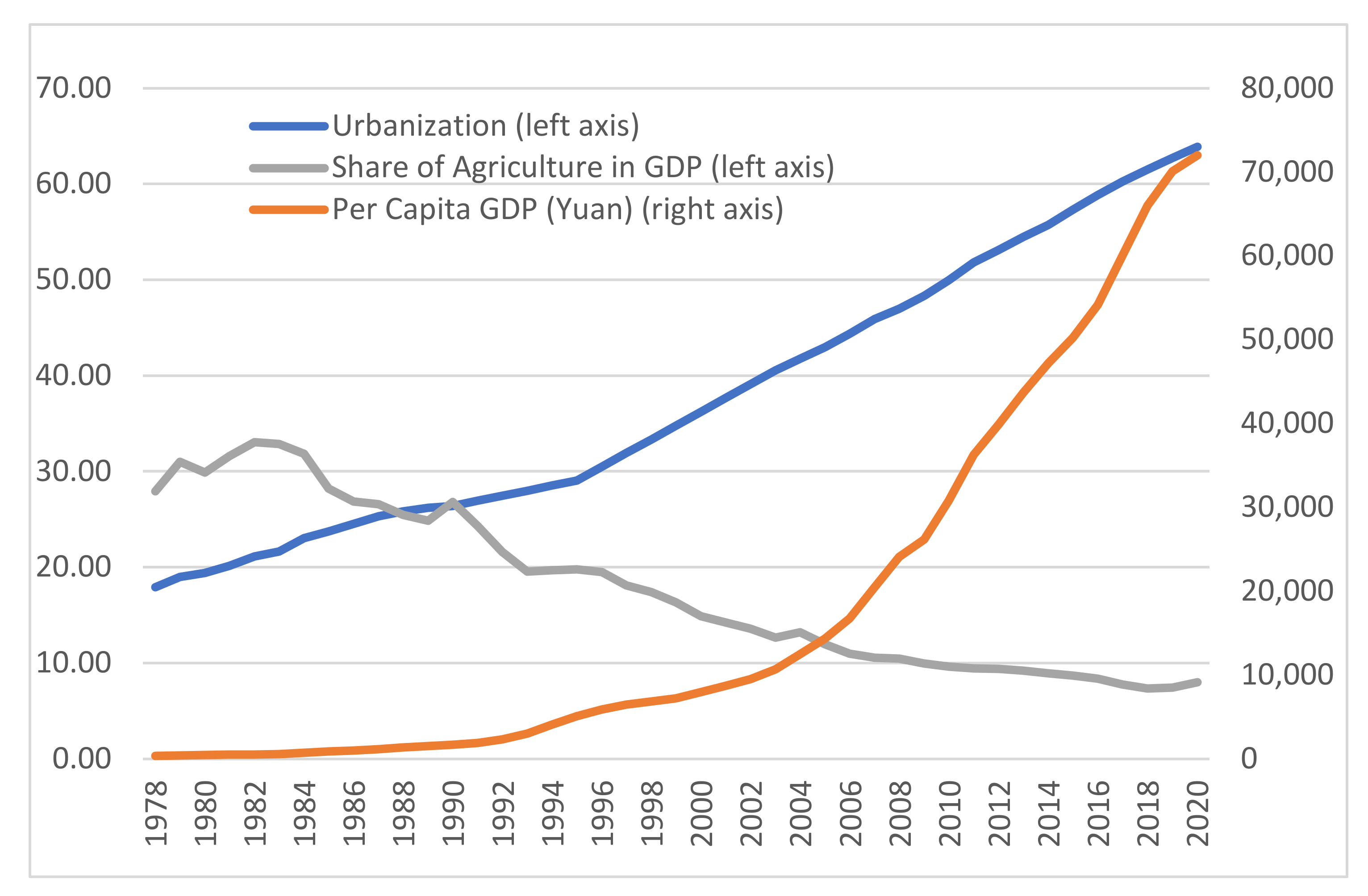
After decades of remarkable economic growth, the urbanization rate in China jumped from 17.92% in 1978 to 63.89% in 2020, with a rapidly expanding urban population (Figure 1). The share of the agricultural sector in total GDP keeps declining, from more than 30% at the beginning of the economic reform to about 7% in 2020. However, as urbanization progresses, there are increasingly worsening sustainability issues across China’s cities, and humans are becoming more involved in the transformation of the natural environment. Urbanization has a profound impact on the ecological environment. Zhou et al. [4] found that urban areas in China as a whole became less green, warmer, and had exacerbated PM2.5 pollution. However, environmental impacts differed in newly developed versus older areas of cities. Urbanization also changes the land use, such as conversion of arable land and grassland to urban construction projects [5,6]. Ecological environments, such as vegetation cover, are thus severely impacted by these human activities.

On the one hand, due to human myopia and ignorance, the idea of prioritizing urban construction has plundered natural resources to some extent and caused a series of short-term behaviors that have largely damaged the environment [7]. On the other hand, people’s desire for a better living environment has prompted active measures to restore ecosystems and promote urbanization rates while seriously taking environmental protection into account. In rural areas, the land could be consolidated and more efficiently used. As such, the net impact of urbanization and human activities on the ecological environment is difficult to deduce simply.

Our study will particularly examine the impact of urbanization upon vegetation cover, as a proxy for the ecological environment, in China, with consideration of both climatic and socio-economic factors. This paper is organized as follows: we will first review the literature in Section 2, then introduce conceptual methods, data, and an econometric model, respectively, in Section 3, Section 4 and Section 5. Section 6 discusses the estimation results, and Section 7 draws conclusions and discusses policy implications.

2. Literature Review

Zhou et al. [4] suggested that the impact of urbanization on the ecological environment is multi-scale and complicated, after using an EVI indicator, an index for canopy structural variations, to measure environmental quality. The literature already uses vegetation cover as a measure of environmental quality, and proposes different conclusions on this topic. In addition to human activities, as part of the natural process, the vegetation cover of a given region is largely limited and influenced by climatic conditions, mainly by temperature and rainfall. Geographically, China’s urbanization rate exhibits a clear ladder structure, decreasing from east to center to west. This is consistent with the geographical distribution of agricultural and rural development levels, which is higher in the east and lower in the west [3]. Interestingly, the natural ecosystems and vegetation in China also follow similar geographical spatial patterns. From east to west, not only does the terrain gradually becomes higher, and the annual precipitation gradually lower, but a transitionary trend from warm and wet to cold and dry is observed. From southeast to northwest, limited by the terrain structure and atmospheric circulation, the ecological sensitivity and vulnerability gradually increase [8].

Researchers have studied the effects of urbanization upon the environment, especially on vegetation cover, in terms of both natural and anthropogenic factors. Some researchers have examined the effects of urbanization on vegetation cover based on climatic conditions (e.g., temperature and precipitation) and social activities [9,10,11], despite economic factors. They argue that climate is the dominant factor for vegetation variation on the whole ecosystem and that social factors (including urbanization and agricultural development) only act on local vegetation cover [7,12]. However, Qu et al. (2020) found that an eco-restoration project, which is representative of social activities, largely promoted vegetation cover on the Loess Plateau. These studies might have ignored the impact of economic activities on vegetation cover, an important indicator for ecological environment.

The literature accounting for both natural factors and human economic activities comes to a more consistent conclusion: the impact of urbanization on vegetation cover still remains unclear, or has no significant effect [13]. Zhou et al. [4] found that urban areas in China as a whole became less green. However, the level of economic development plays a statistically significant role in vegetation cover. There are still significant differences between these studies: the choice of variables representing the urbanization rate differs slightly. Strictly speaking, urbanization refers to the ratio of urban population to total population, which can also be called population urbanization. Yet, the nighttime light from satellites is widely used in empirical studies as a representative variable of urbanization. In some sense, this is a measure for the rate of land urbanization. This inevitably leads to slight differences in results due to different measures. It should be noted that the level of urbanization estimated by the nighttime light data is land urbanization, not strictly the ratio of urban population to total population, while it is generally assumed that the land urbanization progresses faster than the population urbanization [14], which also accounts for the bias to some extent.

Meanwhile, in the studies where variables representing human economic activities are employed, the comprehensive GDP development level has a statistically significant impact on the variation of vegetation cover. Moreover, the estimation shows that the level of human economic development has a significantly positive role in the improvement of vegetation cover, although there are increasing fluctuations across years [15]. This is in line with the findings of official survey reports. According to a report published by National Development and Reform Commission in China, the domestic forest cover for the whole of China increased from 16.55% in 1998 to 21.66% in 2015, the comprehensive cover of grassland vegetation increased from 51% in 2011 to 55.7% in 2018, and deserted land reduces by 1717 square kilometers annually.

Currently, most literature examining the effects of urbanization on vegetation cover are focusing on several major ecologically vulnerable areas in China which are now well protected and under priority restoration construction, namely the Great Green Wall [6], Qinghai-Tibet Plateau [16], Loess Plateau [15], and Yangtze River Ecoregion [17], etc. Or, studies are confined to a particular province [18]. However, to the best of our knowledge, the impact of urbanization on vegetation cover across the whole of China lacks sufficient attention.

Beyond the direct impact of urbanization on vegetation coverage, urbanization also has profound impacts, such as those on agriculture and animal habitat. Wiegand et al. [19] used the NDVI index to measure the habitat quality of animals. Koemle et al. [20] studied the impact of highway construction, which is also related to urbanization, on animal habitat in Austria. Li et al. [3] and Koemle et al. [21] also looked at the linkage between agriculture production, urbanization, and environmental protection.

The rest of the paper will specifically scrutinize the impact of urbanization on vegetation cover, measured by NDVI, in China, while controlling for some economic and climate variables.

3. Conceptual Methodology

The method used in our analysis for estimating the impact of urbanization upon vegetation cover with the NDVI (normalized difference vegetation index) indicator is exhibited in Figure 2. NDVI has been widely used in the literature for measuring vegetation coverage and ecological environment [19,22,23]. We first have an overview of definitions and measurements for urbanization rate, economic development, and NDVI nationwide. Then the marginal effects of urbanization and economic development are evaluated separately by econometric models. Finally, the optimal econometric model is selected by comparing the results of multiple models. Figure 2 shows the main variables, model structure, and logic framework for this research.

3.1. NDVI Indicator

The NDVI indicator [19,22,23,24] is particularly indicative for the greenness of biological communities. Computed with the formula NDVI = (${\rho }_{nir}$− ${\rho }_{red}$)/(${\rho }_{nir}$+${\rho }_{red}$), where ${\rho }_{nir}$ is reflectance in the NIR spectral band, and ${\rho }_{NIR}$ is the red waveband, it is a proxy to evaluate vegetation cover because of the different reflectance between healthy plants and land. In both rural and urban areas, vegetation plays an important role as a regulator in the ecosystem, especially in maintaining terrestrial carbon balance, improving climate conditions, and increasing net primary productivity, which is a direct indicator of ecological environment. Although NDVI is not a physical property of vegetation cover, it can effectively detect plant growth status and cover at large spatial and temporal scales, and has a high positive correlation with vegetation cover density (high NDVI values correspond to high vegetation cover). Thus, at present NDVI is widely used in monitoring and evaluating vegetation cover. As for the NDVI representing vegetation cover in the study, specific values were needed, which required the extraction of NDVI values for each province from the provided NDVI images according to the corresponding geographical location of each province in China from 1998 to 2019.

3.2. Marginal Effect with Interaction

To eliminate the individual heterogeneity effect of each sample on regression results, a fixed effects model was used in our study. An equation of estimating vegetation variation by fixed model can be written as follows:

$$y=ax+bz+cxz+u$$

(1)

where x and z are variables denoting the levels of urbanization and economic development, respectively, while $u$ is a random error term. a, b, and c are related coefficients. According to Equation (1), the marginal effect of urbanization level is:

$$\frac{\partial y}{\partial x}=a+cz$$

(2)

where z is included in Equation (2), that is, the marginal effect of x depends on the value of z. z determines whether the marginal effect is greater than 0 or not. Similarly, we can derive the marginal effect of economic development level:

$$\frac{\partial y}{\partial z}=b+cx$$

(3)

where b, combined with c and x, determines the magnitude of its marginal effect. Equation (3) indicates that the marginal effects of economic development level vary with different stages of urbanization, as does Equation (2).

4. Data and Descriptive Statistics

A large body of literature suggests that the combination of natural and social-economic factors, in some sense, is the main reason for the ever-increasing NDVI and drives the large spatial variation in NDVI dramatically [25]. Natural factors, such as those mentioned in much of the literature, can be generally represented by temperature and precipitation variables, while for social-economic factors, in addition to the level of urbanization, which is closely linked to vegetation, GDP per capita can be used as an essential decisive variable.

Changes in vegetation cover are not only influenced by natural factors, but also depend on human activities. Whether to include the level of urbanization and economic development in addition to natural factors has already been explored in the preceding part. A large body of literature evidences that variations in vegetation cover seem a synergistic impact of climate change and social-economic activities. Therefore, we chose urbanization rate and GDP per capita as representative variables to empirically study the impact of human activities on vegetation cover from 1998 to 2019 which is the key period of rapid urbanization. A total of 22 years of urbanization rates, GDP, population, and CPI indices were collected from 31 provinces, autonomous regions, and municipalities in China to examine the impact of human activities on vegetation cover more accurately and comprehensively. These data come from the China Statistical Yearbook, and the data for 2019 are the latest published by the National Bureau of Statistics to date.

The explanations and descriptive statistics of each variable are reported in

Table 1. Key variables and descriptive statistics.

Symbol	Variable Definition	Obs.	Max	Min	Mean	SD
Dependent variable
NDVI	Normalized difference vegetation index	682	0.916	0.166	0.662	0.169
Independent variables
UB	Urbanization rate	648	0.896	0.174	0.491	0.159
PGDP	GDP per capita (10,000 yuan)	682	10.748	0.235	2.436	1.849
Control variables
temp	Average annual air temperature (°C)	670	25.80	3.50	14.41	5.07
rain	Accumulated annual precipitation (mm)	670	9364	74.90	919.60	624.55

Data source: Authors’ calculation based on the China Statistical Yearbook (1998–2019) and CLGS.

.

4.1. Urbanization

Human activities are mainly reflected in social and economic aspects. The urbanization rate is used to reflect human social activity. In the development stage, rapid growth of urbanization in some regions is accompanied by increased demand for urban construction land and destruction of vegetation under the tension of human–land conflict [4,5,7,20]. However, it is difficult to draw a unified conclusion on the effect of urbanization on vegetation cover because of the complex relationship between them [3]. Based on the preceding analysis, this paper uses population urbanization rate as the indicator representing overall urbanization progress.

4.2. GDP Per Capita

GDP per capita is applied to objectively reflect the level of local economic development and economic activities. Due to the differences in size and population between provinces and cities, GDP per capita is a superior indicator for actual economic development level, or the wealth level for a region.

Because the data have a span of 22 years, the real GDP of each province is obtained by dividing the nominal GDP of each province by the GDP deflator of the year in which it is located, where the CPI of each year is used as an approximation of the GDP deflator. In particular, the logarithm of real GDP per capita (lnPGDP) is used to measure the economic development of each province.

The trends of GDP per capita and urbanization rate are depicted in Figure 1. Both of them behave in increasing trends throughout the sample period. Specifically, there is an obvious surge in GDP per capita after 2002 nationwide. An important reason could be that China entered the WTO in 2001, and was further integrated into the global market.

4.3. NDVI

The data for the NDVI comes from the website of Copernicus Global Land Service (CGLS) (Sources:Copernicus Global Land Service. https://land.copernicus.eu/global/products/ndvi (accessed on 26 November 2021)), which provides geophysical products on land surface conditions and evolution under the European flagship program on Earth Observation at the global scale over long periods of time.

CGLS provides global NDVI data at multiple spatial and temporal scales, updated every 10 days, with the earliest NDVI data starting in 1998, when our sample data begins.

Furthermore, based on the characteristics of China’s climatic conditions and surface plant growth cycle, we selected the NDVI data from August 1 to 10 each year, which is almost the most vigorous period of plant growth, to represent the annual vegetation cover. Specifically, a collection of NDVI 1km is used in our study, and all NDVI data in the whole period are consistent in the same scale and dimension.

The NDVI provided by CGLS, however, is not presented as a number, and thus the average value of each province needs to be extracted separately for different provinces. This step is repeated continuously to collect panel data of 31 administrative units in China from 1998 to 2019 along with other variables. Considering the close relationship between NDVI and vegetation cover, this study employs the logarithm form of NDVI (lnNDVI) to estimate the vegetation cover in each province over time.

Figure 3a–f depicts the overall NDVI trend images for 31 administrative regions of China every four years from 1998 to 2019. According to the trend of urbanization and GDP per capita in Figure 1 and NDVI in Figure 3a–f, the following straightforward conclusions can be drawn. First, NDVI changes occur in a complicated manner rather than following a stable trend. Granted, China’s urbanization rate and GDP per capita show a yearly upward trend, but the change in NDVI is not linear. Although nationally vegetation cover performed much better in 2019 than in 1998, we can observe some fluctuations in between.

Clearly, the urbanization process is often accompanied by rapid economic growth, as the rural laborers move to urban areas to earn higher income. It implies that there is an interaction effect between them.

4.4. Other Control Variables

Temperature and precipitation are used as control variables to control for the effect of natural factors (climate change) on vegetation cover. Climatic factors are among the most significant factors in determining the adequate growth of local surface plants, for both general plants and agricultural crops [26,27,28,29]. Especially in certain areas with inclement climate (e.g., Loess Plateau), the vegetation growth level is greatly limited by the natural environment. Generally speaking, the more suitable the local climatic conditions are, the better the biomes grow and the more it is conducive to the increase of vegetation cover. Thus, this study empirically uses the logarithm form of the average annual local temperature (lntemp), and the logarithm form of the average annual rainfall depth (lnrain) to control for the potential heterogeneity of local climatic conditions in multiple provinces. Common sense suggests that high temperatures and droughts are very detrimental to vegetation growth and therefore have the potential to cause negative changes in NDVI. Wang et al. (2015) even found the adverse impacts of drought have offset the benefits of ecological restoration to some extent [29].

5. Econometric Model

In general, the impact of social activities upon ecological environment depends on the attitude of human beings towards nature—for instance, the degree of environmental concern varies among provinces—and this is reflected in the extent to which the natural environment is damaged. In order to control for the provincial heterogeneities, we used a fixed effects model for the panel data. Since the impact of changes in urbanization on NDVI depends on the level of GDP per capita while ensuring that GDP per capita remains constant, for example, provinces with higher GDP per capita may be more aware of environmental protection than the provinces with lower GDP per capita: an interaction term between the two is consequently necessary in the model. This is consistent with the information reflected in Figure 1 and Figure 3a–f.

Taking all these into account, a fixed effects econometric model incorporating the urbanization, GDP per capita, interaction term, and the climate variables, is specified as follows:

$$y_{it}={\beta }_0+{\beta }_1{U}_{it}+{\beta }_2{G}_{it}+{\beta }_3{U}_{it}\times G_{it}+\gamma X_{it}+\delta Z_i+{\epsilon }_{it}$$

(4)

where $y_{it}$ is the NDVI taken as the natural logarithm (lnNDVI), and is the dependent variable to measure ecological environment for province i in year t; $U_{it}$ is the urbanization rate of province i in year t ($UB$) (we did not take the natural logarithm for U_it, because in this original form, we can better explain the coefficient for $U_{it}$, as the impact of the direct improvement of urbanization ratio on ecological environment (NDVI), rather than of the growth rate of urbanization ratio); $G_{it}$ is the natural logarithm of the level of GDP per capita in province i in year t (lnPGDP); the interaction term $U_{it}\times G_{it}$ is used to capture the interaction effect between urbanization and economic development level; $X_{it}$ is a vector of control variables containing the natural logarithm form of temperature and precipitation for province i in year t (lnrain and lntemp); $Z_i$ represents provincial effects; and ${\epsilon }_{it}$ is the error term. ${\beta }_0$, ${\beta }_1$, ${\beta }_2, {\beta }_3, \gamma$, and $\delta$ are corresponding coefficients.

Furthermore, it is worth noting that the signs of the coefficients of the interaction terms represent different relationships between GDP per capita and urbanization rate, respectively. If the coefficient of the interaction term between the two is negative, it indicates a substitution effect between GDP per capita and urbanization rate, whereas when the coefficient of the interaction term between the two is positive, it represents a complementary effect between GDP per capita and urbanization rate.

Random effects models are similar to fixed effects models but they are more efficient. A premise for the use of the random effects model is that the individual effect $Z_i$ is neither correlated with the error term ${\epsilon }_{it}$ nor with any other variable in Equation (1). The fixed effects regression results can be compared with those from the random effects model to test the robustness of the model using the Hausman test (all the estimations were performed byR 4.0) [30].

The literature shows that the effect of urbanization on NDVI is unclear [31]. Again, with our consideration of the presence of interaction term, we regressed all of the variables of Equation (4), and also regressed some of these variables separately, to check the robustness of the results; the FE regression results are summarized in

Table 2. Estimation results of the fixed effects model for NDVI.

Variables	FE (1)		FE (2)		FE (3)		FE (4)		FE (5)
	Coeff.	t-Ratio	Coeff.	t-Ratio	Coeff.	t-Ratio	Coeff.	t-Ratio	Coeff.	t-Ratio
UB	0.1456 ***	4.53	0.1372 ***	4.27	0.0049	0.10	0.0062	0.12
lnPGDP					0.0237 ***	3.28	0.0728 ***	4.58	0.0734 ***	4.94
UB*lnPGDP							−0.0946 ***	−3.46	−0.0946 ***	−3.46
lntemp			−0.1001 **	−2.29	−0.0954 **	−2.18	−0.0899 **	−2.07	−0.0897 **	−2.07
lnrain			0.0348 ***	2.99	0.0333 ***	2.87	0.0385 ***	3.33	0.0386 ***	3.34
Individual effect	No		Yes		Yes		Yes		Yes
R2	−0.0164		0.0034		0.0192		0.0315		0.0383
F-test	20.5449 ***		11.7176 ***		11.6119 ***		11.1372 ***		14.841 **
Observations	682		682		682		682		682

Note(s): *** and ** denote 1% and 5% statistical significance, respectively.

. Each column in Table 2 reports a corresponding form of regression.

6. Results

6.1. Estimation Results

Three salient conclusions can be inferred from Table 2. According to the regression results of FE (1) and FE (2), neither control variables nor other variables are included in FE (1), and an inclusion of control variables (log temperature and log rainfall) causes the coefficient on UB in FE (2) to drop from 0.1456 to 0.1372, but this remains statistically significant at the 1% level.

Second, statistical significance of urbanization (UB) disappears after including lnPGDP. It is clear evidence of an interaction effect between economic development and urbanization as they are highly correlated. FE (3) is the regression result of the equation after adding the logarithm form of the PGDP variable to FE (2), and the coefficient changes dramatically, dropping from 0.1372 to 0.0049, which is close to 0. In particular, the coefficient on UB is no longer statistically significant. In other words, the regression results indicate that urbanization is neither statistically significant nor economically important in this setting. In contrast, the newly added variable (lnPGDP) becomes statistically significant at the 1% level, which suggests that the logarithm form of PGDP explains a large portion of urbanization in the equation, and economic development level and urbanization are correlated.

When the interaction term between GDP per capita and urbanization rate are considered, the results in FE (4) are given in Table 2. As expected, the UB coefficient changes slightly but in neither FE (3) nor FE (4) is the coefficient significant even at the 10% level, and the term UB should be consequently dropped. The interaction term is statistically significant at the 1% level with a negative coefficient in the estimates of FE (4), which implies an offsetting effect between UB and lnPGDP. Additionally, an F test further rejected the null hypothesis of a zero coefficient on the interaction term at the 1% significant level with p-value of less than 0.001.

The coefficient for InPGDP indicates the same significant level as FE (3) though the coefficient increases a little bit. The inclusion of the interaction term makes the marginal effect of lnPGDP depend not only on itself but also on the value of UB, which proves that regions with identical PGDP are different for various levels of urbanization rates.

To sum up, dropping UB and including all other remaining variables was seen to be the optimal regression function because NDVI is not sensitive to the urbanization rate itself. Thus, the regression of FE (5) is modified based on regressions FE (1) through FE (4), and the estimates reported in the column labeled FE (5) are very similar to the ones in FE (4). This justifies the composition of variables in the regression function. Therefore, Equation (4) is modified as follows:

$$y_{it}={\beta }_0+{\beta }_2{G}_{it}+{\beta }_3{U}_{it}\times G_{it}+\gamma X_{it}+\delta Z_i+{\epsilon }_{it}$$

(5)

Estimates of vegetation cover by stepwise inclusion of the variables UB, lnPGDP, UB $\times$ lnPGDP, and control variables are presented in Table 2, and column FE (5) gives the estimation results of the optimal model of Equation (5) with all variables having significant impact on vegetation cover.

6.2. Robustness Check

Equation (5) can be estimated either by a random effects model, a fixed effects model, or a pooled regression model, because Equation (5) is based on a set of panel data. By regressing Equation (5) based upon these three different models we can make a straightforward comparison between regression results, as presented in

Table 3. Estimation results of the different regression models for NDVI.

Variables	FE		RE		Pooled
	Coeff.	t-Ratio	Coeff.	t-Ratio	Coeff.	t-Ratio
lnPGDP	0.0734 ***	4.9373	0.0740 ***	4.9312	0.0505	1.212
UB*lnPGDP	−0.0946 ***	−3.4639	−0.0956 ***	−3.4708	−0.0094	−0.145
lntemp	−0.0897 **	−2.0722	−0.0364	−0.8817	0.1438 ***	3.949
lnrain	0.0386 ***	3.3365	0.0456 ***	3.9349	0.2616 ***	11.161
Control variables	Yes		Yes		Yes
R2	0.0383		0.0785		0.387
F-test/Chi2	14.841 **		58.773 ***		101.2 ***
Observations	682		682		682

Note(s): *** and ** denote 1% and 5% statistical significance, respectively.

. Entries in columns labeled FE and RE represent regression results of the fixed effects model and the random effects model, respectively, but they are very similar in terms of numerical magnitude and statistical significance levels. This also provides some evidence for robustness of our results. However, further validation should come from the results of an F-test and Hausman test.

The choice of model will be subject to the test results. These tests are used to make sure that individual effects are significant, that is, that heterogeneity is significant. If the heterogeneity is very significant, then the fixed effects model is preferred, rather than the pooled regression model, and vice versa [32]. If there is no evidence indicating a systematic difference in samples, a random effects model would be employed, because it has a characteristic of efficiency superior to a fixed effects model, which is always consistent but is not efficient. Otherwise, a fixed effects model is preferred, because it is always consistent. Specifically, an F-test can be used to examine the systematic differences among provinces between pooled regression and a fixed effects model, while a Hausman test could be used to test significant heterogeneity between a random effects model and a fixed effects model. The test results are summarized in

Table 4. Estimation results of F-test for individual effects.

F Value	p-Value	Result
289.8	0	Significant effects

and

Table 5. Estimation results of Hausman test.

Chi2	p-Value	Result
15.827	0.0033	One model is inconsistent

.

This shows a significant result (at a 1% statistically significant level) from the F-test between the pooled regression and the fixed effects model, indicating that the fixed effects model is preferred, since there are obvious systematic differences among provinces. Similarly, Table 5 also presents the result for the same level of significance, suggesting a fixed effects model is superior to a random effects model because the Hausman test rejected the null hypothesis of no systematic difference between the FE and RE models. Therefore, overall, among these test results, the fixed effects model outperforms both the pooled regression model and the random effects model, and thus it is reasonable to employ the fixed effects model in Equation (5), and the estimation results in Table 2 is consequently robust.

7. Discussions

• Urbanization effect

This is contrary to our initial assumption: urbanization has a significantly negative impact upon vegetation cover. The higher the urbanization ratio is, the larger the negative impact is. It implies that urban expansion does reduce ecological environment. However, the magnitude of marginal effect depends on the income level. The higher the income is, the larger the marginal effect is in terms of absolute values.

• Income effect

We now take a look at the income effect measured by the per capita GDP. In particular, according to the last column, the marginal effect of lnPGDP, 0.0734–0.0946$\times$UB varies with the value of UB. For UB < 77.59%, Equation (2) is an increasing function of lnPGDP, thus the value of lnNDVI increases as GDP per capita grows in this range, and thus the positive changes in PGDP are accompanied by wider vegetation cover. For UB = 77.59%, whatever changes in PGDP will have no impact on NDVI. For UB > 77.59%, positive changes in GDP per capita will decrease vegetation cover.

$$\mathrm{Marginal} \mathrm{Effect} \mathrm{of} \mathrm{l}\mathrm{n}PGDP: \{\begin{array}{c}> 0,UB < 77.59\%\\ = 0,UB = 77.59\%\\ < 0,UB > 77.59\%\end{array}$$

This suggests that raising the level of GDP per capita in areas with low urbanization rates will help a lot to promote vegetation cover, but it will decrease the NDVI beyond the threshold (if UB ≥ 77.59%). There are probably two reasons for this result. First, in the initial stage of urbanization, part of the increase in GDP per capita came from farmers moving to the cities to work, with their farmland being thus consolidated or abandoned and entering the natural ecosystem, becoming part of the rewilding process [20,21,33]. The other is that in this primary stage, the increase in GDP per capita raises the awareness of environmental protection in local areas, and the marginal effect is greater at this stage when the overall economic improvement and regional development make it possible to invest more in an increase in greening areas and active afforestation activities.

The result is consistent with Shi et al. (2020) [34], who found, by using a machine-learning method, that the vast majority of the increase of NDVI could result from human activities, in some regions the contribution effect being more than 100%, with the rest being highly associated with climatic factors. Moreover, according to official reports, China has carried out a series of ecological projects and invests a lot of human and material resources in order to strengthen the construction of ecological civilization, and the ecological quality has continuously improved in vital areas [6]. For instance, Sanjiangyuan, which is known as the Chinese water tower, has received more than 17 billion yuan of investment for its restoration project since 2005, and the second phase of the project amounts to 10 billion yuan. After more than ten years of restoration and improvement, the vegetation cover of the local grassland has reached 74%, and the vegetation cover of the deserted land has increased from 33.36 to nearly 40%. Apparently, large scale economic inputs have extraordinarily contributed to vegetation cover restoration (Sources: Chinese central government. http://www.gov.cn/xinwen/2018-06/20/content_5299871.htm (accessed on 12 December 2021)).

For areas with a high urbanization rate, the expansion of urban scale is prone to the phenomenon of crowding out rural vegetation cover owing to the prominent contradiction between humans and land, and to the fact that the demand for land for urban development and construction is difficult to satisfy in cities. For instance, in the Yangtze River Delta region, which has a high urbanization rate, the intensity of land development is close to the maximum [5,15].

Meanwhile, noteworthy is the interaction term between GDP per capita and urbanization on NDVI, whose impact is negative, which is not only statistically significant but also of much practical importance, indicating that a high level of average economic development in provinces with low urbanization rates leads to increased vegetation cover. By contrast, a highly developed economy in a more urbanized province results in decreased NDVI. That is, the positive marginal impact of GDP per capita on vegetation cover will decay with the increase of urbanization rate. In other words, there is a counteracting effect between lnPGDP and UB, as mentioned before.

Nevertheless, 77.59% is a very high level of urbanization rate, representing 77.59% of the total population in urban areas. The current (2020) urbanization rates of several countries are 63.89% in China, 82.66% in the United States, 91.78% in Japan, 81.41% in Korea, and 77.45% in Germany (Data source:https://www.statista.com/search/?q=urbanization&Search=&qKat=search&language=0&p=2 (accessed on 25 December 2021)). It seems that the developed countries worldwide are marked by a high rate of urbanization, and it will take some time for China to become a country with a more than 77.59% urbanization rate. Some developed countries, such as Germany, had an urbanization rate of over 70% by the middle of the last century. China, as a developing country, which is at a medium level of urbanization, aims for an urbanization rate of 70% by 2030.

Although China’s current urbanization level does not reach 77.59%, it presents a significantly higher level of urbanization in the eastern coastal provinces than in the western and central regions due to its highly uneven development among domestic areas. The data for 2020 show an urbanization rate of 89.3% in Shanghai and 74.15% in Guangdong, compared with 35.73% for Tibet and 50.05% for Yunnan. Furthermore, in the 1980s, some highly polluting industrial enterprises entered the rural areas, thus their industrial waste and urban garbage seriously damaged the rural environment. Meanwhile, the mushrooming of township enterprises improved the income level of farmers, but also intensified the destruction of the rural ecological environment.

Although several national environmental protection policies were introduced in the late 1990s, it was not until the early 21st century that the central government spared no effort to combat pollution through multiple means [35]. Peng et al. (2011) also point out that NDVI varies with seasons and ecosystems [36], and northern China is more affected by temperature and drought compared with southern China, thus NDVI shows a decreasing trend. As such, it is reasonable that Figure 3a–f show inconsistent NDVI trends for different periods in different provinces, which have high correlation with each province’s own urbanization rate and attitude towards pollution, and the strength of policy implementation at different times.

The overall urbanization rate in China is currently well below the turning point of 77.59%. Adherence to the current development path in most provinces could maintain vegetation cover without degradation.

However, an increase in vegetation cover or NDVI does not merely mean that the environment is well protected, nor does it mean that humans’ activities are in harmony with the natural landscape. The massive influx of rural people into cities has brought about the consolidation of agricultural land, abandonment of large areas of farmland, and decrease in economic activities in environmentally vulnerable areas. Gradually, the abandoned farmland has merged into the local natural landscape and become part of the vegetation cover, but the villages are also decaying as a result. This corresponds to the first reason why economic growth in low-urbanized areas is accompanied by an increase in vegetation cover, as analyzed in the preceding part.

8. Conclusions and Policy Implications

The relationship between urbanization and ecological environment is not conclusive in the literature. We used the provincial data from China between 1998 and 2019 to empirically study the relationship between urbanization ratio and ecological environment which is proxied by NDVI from the remote sensing data. It is widely known that economic development is highly correlated with urbanization: high urbanization implies a high level of economic development. In an econometric model, we have to include the interaction between economic development level and urbanization. First, the coefficient of the interaction between urbanization and per capita GDP is statistically significant and negative, while the coefficient of urbanization itself is very small and not statistically significant. It implies that urbanization could reduce ecological quality, particularly for high-income regions. The higher the urbanization ratio is, the larger the negative impact is. It implies that urban expansion does reduce the ecological environment.

The effect of GDP per capita on NDVI can be divided into three stages: the one where the NDVI improves with the increase of GDP per capita (an urbanization rate of less than 77.59%), the one where the value of the NDVI is not affected by the level of GDP per capita (an urbanization rate equal to 77.59%), and the one where the NDVI decreases with the increase of GDP per capita (an urbanization rate of more than 77.59%).

Currently, the urbanization rate in the vast majority of provinces of China is well below 77.59%, the high degree of urbanization commonly found in developed countries worldwide. In this scenario, most provinces in China are in the first stage: an increase in local GDP per capita is accompanied by an improvement in the NDVI. Notably, this does not mean that economic development can march at the expense of the natural environment. This can be explained by the national awareness of environmental protection, enhanced with the improvement of the economic development on the one hand, and part of the arable land becoming consolidated or merged into rewilding places as a result of farmers moving into the city for work on the other hand.

In addition, Chinese governments have stepped up efforts to protect the environment and have increased dedicated funds for environmental protection since the beginning of the 21st century, which has achieved the intended results to some extent. With a series of powerful policies in place, China has shifted the focus from solving pollution problems in a single area to coordinating the balanced development of the whole society and started to put an emphasis on a sustainable development model. This could greatly contribute to vegetation cover increase and comprehensive environment improvement. Hence, this can be seen as an experience practiced by developing countries (e.g., India and most African countries) in the stage of low urbanization rate to achieve the positive effect of economic growth on vegetation cover.

Although economic growth in most provinces has contributed to the increase in vegetation cover, attention should also be paid to regions at the opposite stage, where economic development has a negative impact upon vegetation cover. The conflict between humans and land is more prominent in highly urbanized areas with more limited urban construction land, which might do harm to vegetation cover. As such, balancing the opposite effects of economic development on vegetation cover in different geographical regions in the same country requires more effort and attention.