Abstract
Intensity-duration-frequency (IDF) curves representing the variation of the magnitude of extreme rainfall events with a return period and storm duration are widely used in hydrologic infrastructure design, flood risk management projects, and climate change impact studies. However, in many locations worldwide, short-duration rainfall-observing sites with long records do not exist. This paper introduces a new methodological framework for extracting IDF curves at ungauged sites transferring information from gauged ones with a relatively homogeneous extreme rainfall climate. This methodology is grounded on a simple scaling concept based on the multifractal behaviour of rainfall. A nonstationary Generalized Extreme Value (GEV) distribution fitted to annual rainfall monthly maxima at the ungauged site using a moving-time window approach is also applied to consider effects of a changing climate on IDF curve construction. An application is presented at the study site of Fourni, Crete, to derive IDF curves under changing climate conditions and present implications of the proposed methodology in the design of a sustainable stormwater network. The methodology introduced in this work results in increased rainfall extremes up to 20.5%, while the newly designed stormwater network is characterised by increased diameters of its primary conduits, compared to the ones resulting under fully stationary conditions.
1. Introduction
Extreme rainfall events can cause damaging floods around the globe and therefore constitute an important problem in hydrologic risk analysis and design or management of critical infrastructure. Estimation of extreme rainfall for a given duration and a selected return period is therefore necessary for the planning and design or management of many hydraulic structures (i.e., dams, reservoirs, detention ponds, bridges, roads, storm sewers, pumping stations and culverts), as well as for inundation risk mitigation. The general inception of a changing climate with extreme meteorological events of higher intensity and frequency increases vulnerability and exposure of human societies to flooding and of stormwater and urban drainage systems to failure risks. Neglecting such effects in the design of stormwater networks can significantly increase flooding risks and have devastating effects on all flood risk receptors.
Intensity-Duration-Frequency (IDF) curves summarise the relationship between rainfall intensity, duration, and probability of exceedance expressed by the return period of the event. Such curves are currently utilised for hydrological infrastructure design and management applications, flood risk management for assets and infrastructure, or flood mitigation projects [1,2,3,4,5,6,7,8]. IDF curves are constructed for different return periods representing the variation of rainfall intensity with duration. They are usually constructed by fitting theoretical probability distribution functions to annual maximum rainfall intensities of durations ranging from shorter ones, that is, sub-hourly to daily, or even larger duration rainfall events.
Extreme value analysis methods are currently used worldwide to estimate IDF curves with reasonable accuracy for sites possessing long records of short-duration rainfall [5,8]. However, in many parts of the world, there exist many partially gauged or ungauged sites, where construction of IDF curves is necessary for different engineering or management applications. For such partially gauged or ungauged sites, regional frequency analysis (RFA) is currently used to construct IDF curves in most studies [9,10,11]. RFA uses information from gauged sites in a region considered homogeneous in terms of its extreme rainfall climate and transfers this information to ungauged sites [9,10,11]. El-Sayed [12] used iso-pluvial maps to derive regional IDF curves in a selected area in Egypt. Liew et al. [13] used bias-corrected records from nearby meteorological stations to derive IDF curves at ungauged sites in Malaysia. Major concerns in RFA studies constitute the delineation of homogeneous regions [14,15], as well as the transferring of information from a defined homogeneous region to the ungauged site [16,17,18,19]. For the latter, two quantile estimation methodologies are most used, namely, the index-flood or index-storm approach, and the at-site regression approach [9,16,18]. In the latter, an ordinary least-square (OLS) regression model with physiographic and climatic predictors is used within a delineated region to estimate the at-site quantiles. To overcome the main deficiencies of the OLS regression model, which summarise the unreliable estimates of at-site quantiles at locations without short-duration rainfall measurements, linear and nonlinear quantile regression models which directly link physiographic and climatic predictors to extreme values of rainfall in a homogeneous region have been proposed [20,21]. Ouali and Cannon [22] proposed a regional framework based on quantile regression to estimate IDF curves at ungauged sites, also investigating the added value of nonlinear methods for modelling RFA relationships.
IDF curves are currently designed under the assumption of stationarity [23,24,25], namely the hypothesis that the occurrence probability of precipitation events will remain unaltered or will not exhibit significant changes in time. However, the fact is that such hydro-meteorological signals, especially at their extreme levels, exhibit phenomena of nonstationarity [26]. Natural climatic variability, human interventions in the hydrologic cycle of different catchments areas, and climate change are some of the prominent causes of such nonstationarities [27]. To incorporate nonstationarity in modelling extreme values of a process, different approaches have been considered in the literature. Such statistical approaches consider probability distribution functions, including parametric trend components, non-parametric models incorporating covariates varying with time, stochastic models with shifting patterns, and probability distributions with mixed components. Kharin and Zwiers [28] used parametric extreme value models with time-dependent parameters to estimate extremes in transient climate change simulations. El Adlouni et al. [29] incorporated a climate covariate, namely, the Southern Oscillation Index (SOI) in the analysis of extreme precipitation by means of a parametric nonstationary extreme value model. Cooley [30] reviewed some extreme value analysis techniques used to assess the impacts of climate change on hydro-meteorological extremes and analysed extreme temperatures in central England, using parametric nonstationary extreme value models. Towler et al. [31] utilised the nonstationary generalized extreme value (GEV) distribution with its parameters varying as parametric functions of climate covariates to analyse hydrologic and water quality extremes in a changing climate. Cheng et al. [32] introduced a framework for modelling nonstationary extremes using Bayesian inference and constructed a software package (NEVA) to perform their analysis. Cheng and AghaKouchak [5] utilised the aforementioned methods and tools to estimate nonstationary IDF curves. Ganguli and Coulibaly [26] examined trends and nonstationarity in short-term precipitation extremes and evaluated the potential of nonstationary IDF curves in Southern Ontario, Canada. Sarhadi and Soulis [33] presented a fully time varying framework based on Bayesian inference to incorporate climate change effects on the occurrence of extreme precipitation in the Great Lakes area. Agilan and Umamahesh [34] used multi-objective genetic algorithms to model nonlinear trends in parameters of extreme value models for rainfall and utilised them in the construction of nonstationary IDF curves. Ouarda et al. [35] developed nonstationary IDF curves in Canada expressing their parameters using climate oscillation indices and time covariates. Silva et al. [36] assessed future nonstationary IDF curves in Canada using equidistance quantile matching methods. Yan et al. [37] updated current IDF curves using nonstationary modelling of extreme precipitation including physically-based covariates and downscaling methods for projection purposes.
Rainfall time-series of fine temporal scales are essential for the construction of IDF curves, as well as for studying climate change effects, especially on medium or small-scale catchments. However, the lack of short-duration rainfall measurements at many sites worldwide (ungauged or partially gauged sites), as well as rainfall resulting from climate models, complicate the modelling of both the precipitation and the sewer processes. Temporal downscaling and temporal disaggregation are used to overcome such difficulty [11,38,39,40,41,42,43,44,45,46]. Temporal downscaling usually refers to the generation of data of high temporal resolution by means of statistical techniques, most commonly, scaling techniques or stochastic models calibrated using information on the statistics of data from lower resolution temporal scales [38,39,40,41,42,43]. Scaling approaches currently used for rainfall include simple scaling [38,39,40], as well as multiscaling [42,43] techniques. Bara et al. [44] estimated IDF curves in Slovakia using a simple scaling approach within a regional analysis framework. Ghanmi et al. [45] combined simple scaling invariance of annual maximum rainfall intensities with the Gumbel distribution function to develop a regionalisation formula and estimate IDF curves for northern Tunisia. Yeo et al. [46] compared three fitting methods for scaling the GEV distribution function in terms of their ability to temporally downscale daily annual maximum precipitation to be used in the design of IDF curves in two distinct climate regions in Canada and South Korea.
Small temporal and spatial scales of hydrological processes in urban areas hinder the different studies of climate change impacts on such catchments. However, such studies are extremely important, especially nowadays, because of the increasing frequency and intensity of urban storms due to climate change and of their significant consequences to human life and health, the society, the economy, and the environment. It should also be noted that climate change effects on hydrological processes of urban catchments can be significantly affected by land use changes, and especially by the increasing number of impervious surfaces in such areas. Willems et al. [47] presented the state-of-the-art methods for assessing the impacts of climate change on precipitation at an urban basin, suggesting an upgrading of the pipe systems with insufficient capacity over the next few years. Arnsbjerg-Nielsen et al. [48] highlighted the importance of studying climate change effects on rainfall extremes and urban drainage infrastructure, focusing especially on the design and optimisation of urban drainage systems. Langeveld et al. [49] studied the effects of climate change on urban wastewater infrastructure, revealing weak parts of the system under future conditions and limited knowledge on sewer processes. Willems [50] revised the urban drainage design rules in Belgium taking into account the precipitation extreme trends until the end of the century. The urban drainage storage facility was modelled by a continuous reservoir simulation approach and the impacts were studied for a range of throughflow rates, concluding that an increase in storage capacity is necessary in order to keep the overflow frequency to the current level. Moore et al. [51] developed several climate change scenarios and used the SWMM (US EPA Stormwater Management Model) model to predict flooding in selected urban areas, ending up with examining adaptation options to enhance the resilience of stormwater systems. Kumar et al. [52] evaluated climate change impacts on urban flooding using future precipitation from Regional Climate Models (RCMs) and the SWMM hydrodynamic model, resulting in a future increase of flooding risk in the study areas with respect to present conditions. Huq and Abdul-Aziz [53] developed a large-scale stormwater model for southeast Florida in SWMM to investigate changes in runoff due to simultaneous climatic and land cover changes, detecting an increase in flood risk in urban centers. Kourtis et al. [54] presented a comprehensive review of adaptation options of urban drainage networks to climate change, identifying the main scientific approaches, assessing costs and benefits, and defining a novel approach for the assessment of urban drainage network adaptation to climate change.
IDF curves summarising the relationship between rainfall dynamics, namely intensity, duration, and frequency (return period), are very useful tools for classifying climate regimes, modelling different hydrologic processes, designing urban drainage systems, analysing and managing flood risk in flood prone areas, and assessing impacts of extreme rainfall on catchments. Current IDF curves are based on the concept of stationarity, neglecting the nonstationary characteristics of the climate. However, the evidence of a changing climate, expected to have significant effects on the intensity, the duration, the spatial distribution, and the probability (frequency) of occurrence of extreme precipitation events, emphasises the need for a nonstationary analysis of such events to produce more reliable and robust estimates for the most extreme part of the rainfall distribution. The fact that there exist many sites worldwide where there are no dense networks of short-duration rainfall observations, significantly complicates the construction of IDF curves, and therefore hinders design, analysis, and management of different infrastructure systems. The present work aims at presenting an advanced but rather simple methodology for constructing IDF curves at sites with no short-duration rainfall observations under the assumption of a changing climate. The proposed methodology uses information on the rainfall dynamics from a site with relatively homogeneous extreme rainfall climate with the study site, and produces inference based on the hypothesis of scale invariance of annual maximum rainfall intensities. Rainfall scaling is applied in this work using coarse resolution annual maximum rainfall data at the study site. A nonstationary extreme value distribution is applied to the data available at the study site to account for effects of nonstationarity in the climate system, while the scaling approach is implemented for an appropriately defined time interval of the past climate. Such an approach can significantly affect results of hydrologic and hydraulic design, altering the diameters of stormwater network pipes and therefore modifying the hydraulic bearing capacity of the network.
This work also attempts to introduce nonstationarity inherent in the current climate in the hydraulic design of urban drainage sewer infrastructure. Urban drainage infrastructure is unlikely to be adequate in the future at many sites worldwide because its design relies upon considering stationarity of the past rainfall climate, ignoring climatic variability. However, the assumption of a stationary climate should be abandoned today, highly prioritizing the need for climate variability to be considered. It combines modern and accessible statistical techniques with a well-known and easy to use stormwater hydraulic model, that can be implemented at different urban areas leading to more sustainable designs of the stormwater networks. The methodology presented can contribute to the estimation of IDF curves at sites with no short-duration rainfall observations and therefore to the design or management of critical infrastructure at such locations. The proposed approach can raise the safety level of newly designed urban drainage sewer systems under future climatic conditions, considering that there is increasing evidence nowadays of climate change associated with destructive extreme events of higher intensity and frequency, compared to past conditions. The latter, combined with the rapid deterioration process of the stormwater networks and urbanisation, will result in an increase in the number of people and properties affected by the harmful effects of urban stormwater, imposing the use of innovative and more holistic methodologies in the design process of such systems.
The methodological approach followed in this work is presented in Figure 1.
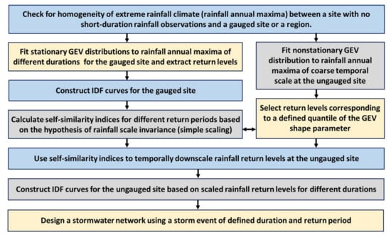
Figure 1.
Methodological approach of the present research.
2. Methodology of the Research
2.1. The Nonstationary GEV Distribution Function
Extreme value theory (EVT) is a robust framework for analysing the tail behaviour of extreme rainfall. Models for block maxima, such as the Generalized Extreme Value (GEV) distribution and for exceedances over appropriately defined thresholds, known as peak over threshold (POT) models, are included within the univariate extreme value family framework. The cumulative distribution function (CDF) of the GEV distribution is given by [55]:
with μ, σ and ξ corresponding to the location, the scale, and the shape parameter of the distribution function. The mean value of the distribution is represented by the GEV location parameter, μ, shifting the distribution left or right. The scale parameter, σ, compresses or stretches the entire distribution and depicts its standard deviation. The GEV shape parameter, ξ, being a measure of the skewness inherent in the data, changes the shape of the distribution. The Gumbel distribution originates from the GEV distribution for ξ = 0. The GEV distribution function unifies the Gumbel, the Fréchet and the Weibull distribution functions into a single family where inference on the shape parameter, ξ, determines the most appropriate type of tail behaviour. A period of one year is usually selected to determine the block size of maxima, and therefore block maxima correspond to annual maxima [55].
Climate change is expected to introduce nonstationarity in variation of extreme rainfall events. Ignoring the nonstationary behaviour of rainfall process can introduce bias in quantile estimates, whereas relatively unbiased quantiles can result from models incorporating covariate effects. Within the extreme value modelling framework, the parameters of the GEV can be expressed as functions of covariates. Consequently, covariates can be used to simulate the extremal behaviour of the studied variable including information on that of another or of several other variables. Considering nonstationarity, the subspace of possible covariates can include the time or any other time-varying variable having some form of impact on the studied phenomenon [56]. To incorporate nonstationarity in Equation (1), the three parameters of the GEV distribution are assumed to vary as functions of time [55]:
Estimates of extreme quantiles exceeded by a probability p can be therefore expressed as:
For the Gumbel distribution function, extreme quantiles can be expressed as:
GEV parameters are estimated using the method of maximum likelihood, most commonly utilised because of its simplicity, its consistency, and its efficiency, especially when the sample size is sufficiently large. Maximisation of the likelihood function with respect to the GEV parameters is numerically straightforward, while maximum likelihood estimators have approximate normal distributions that can be easily used to generate confidence intervals for the GEV parameters [55]. The numerous advantages of the maximum likelihood estimation procedure are seldom subsumed by the fact that due to the numerical structure of the estimator; maximum likelihood estimates can be sensitive to starting values or be biased for small sample sizes whenever numerical stability cannot be attained. For this reason, the L-moments approach [57] is also applied in this work to inspect and verify extracted results of the maximum likelihood estimation procedure. L-moments are usually less influenced by outliers present in the data, while the bias of their small sample estimates has been proven to remain relatively small [58].
In the present work the nonstationary model of Equation (2) has been fitted using a 30-year moving time window shifted by one year each time [59,60]. Therefore, nonstationary GEV (or Gumbel) parameters for the annual maximum rainfall can be assessed for each one of these windows. The length of the moving window is assumed equal to 30 years to obtain a short enough period for the assumption of stationarity to be satisfied and to also obtain an interval of adequate length to fit the extreme value distributions. The derived GEV (or Gumbel) parameter estimates correspond to the last year of each 30-years period and are assessed using the method of maximum likelihood.
Linear and nonlinear parametric trends are then fitted to the extracted GEV (or Gumbel) parameter estimates. The Akaike Information Criterion (AIC) and the Bayesian Information Criterion (BIC) [60], as well as tests for statistical significance of the coefficients of the fitted trends, are utilised here to select parametric trends representing the GEV parameters’ variability in the best possible way. Nonlinear trends include polynomials of order lower than or equal to five. Statistically significant linear trends are judged using the Mann-Kendall test, while F- or t-tests are deployed here for polynomial trends.
2.2. Scaling of Rainfall Intensities
Rainfall features of different temporal and spatial scales can be linked using scaling models relying on the hypothesis of scale invariance [61,62]. Such models are mainly based on the multifractal behaviour of rainfall [24]. Based on the hypothesis of scale invariance, annual maximum rainfall intensities, Id and Iλd, corresponding to durations d and λd, can be related by the following equation [35,44,63], the equality corresponding to similarity of probability distributions:
where λ is the ratio of scale invariance between the known duration, d, and the duration to be assessed, D, and β, is the scale exponent known as the self-similarity index of the process. Strict sense simple scaling is used to describe this behaviour [42,45,61], implying that Iλd and Id are characterised by the same distribution function if finite moments of order q exist for both. The qth moments of rainfall intensity are obtained from Equation (5) after performing the following transformations: (i) raising both sides to an exponent q (order of moment) and (ii) taking averages of both parts [44]:
where β(q) represents the scale exponent of order q, being linear if the relationship between scale exponents and order of moments is linear (wide-sense simple scaling or simple scaling in the broad sense). To estimate β(q), Equation (6) is log-transformed:
The scale exponent β for wide-sense simple scaling can be regarded as the slope of the linear relationship between the log-transformed values of the moments and scale factors for various orders of rainfall intensity moments and therefore be assessed by linear regression. The abovementioned scaling behaviour can also be detected in quantiles of rainfall intensities corresponding to durations d and λd, considering that their CDF has a standardised form independent of the rainfall duration. The CDF of the GEV distribution function, used to model annual maximum rainfall intensities of different time scales, can be expressed in the standardised form:
where F is independent of the rainfall duration, d. This is attributed to the fact that the location and scale parameters, μ and σ, of the GEV distribution depend on d, while the shape parameter, ξ, can be assumed to not vary significantly (assumed almost constant) with rainfall duration [23,38,64].
Simplicity accompanying the application of simple scaling approaches renders them really attractive to be widely used in the construction of IDF curves [38,39,40]. However, for complex physical processes simple scaling seems to deviate from reproducing the probabilistic properties of maximum rainfall intensities. Multiscaling approaches, which involve more than one multiplicative factor in Equation (5) [42,43] seem to better describe the characteristics of such processes. However, in the present work, simple scaling, which rescales maximum rainfall intensity by a constant multiplicative factor, is assumed to adequately describe the scale change of the process. IDF curves at an ungauged site, namely at a site with no short-duration rainfall measurements available (measurements are however available for longer durations), are approximated by the respective curves at another site belonging to a homogeneous region with the one under study with respect to their extreme rainfall climate, using the property of scale invariance of annual maximum rainfall intensity. Simple scaling is implemented in this work, mainly due to the small number of parameters involved in the estimation process (as opposed to multiscaling models), and the hypothesis of scale invariance is applied, considering that annual maximum rainfall return levels for return periods of 2, 5, 10, 20, 50, 100, and 200 years will satisfy the scaling relationship of Equation (7). Self-similarity indices, β, are therefore estimated for each one of the aforementioned return periods, as the slope of the linear regression relationship between the log-transformed values of the quantiles and the scale factors.
2.3. Rainfall IDF Curves
Exploring the relationships that exist between the intensity, duration, and frequency (return period) of precipitation is of particular significance and practicality in hydrologic analysis of urban, semi-urban and rural areas. Rainfall IDF curves are common tools used in water resources management, urban flood risk studies, design of stormwater networks and sewer systems, and management of water supply. Such curves represent links between annual maximum rainfall intensity (or annual maximum rainfall depth) with the return period, T, of a storm event and its duration, d. The general IDF relationship considers that dependence in d and T can be modelled separately [23]:
Such a condition is, however, questioned by Veneziano et al. [62] by processing multifractal rainfall models with theoretically known IDF curves. They proposed marginal distribution and hybrid methods instead, that can model interactions between d and T. However, for simplicity purposes, in the present work, Equation (9) is used to represent the IDF relationship, considering that the main focus is to present a general methodological framework for designing stormwater networks in a changing climate for ungauged sites. The nominator of Equation (9), α(Τ), is given in the literature [65,66,67,68] by the following alternative equations:
where h, c, K are coefficients to be determined by the available data. Equation (11) is the oldest and the most common one, being dictated by its simplicity and computational convenience. Chen [69] applied more theoretical analysis to obtain similar equations. Koutsoyiannis [70] has proven empirically that the parameters K and c of Equation (11) are not stable and depend on the return period T, if maximum rainfall intensity is simulated by a Gumbel distribution function.
The denominator of Equation (9) is determined as [45]:
with θ ≥ 0 and 0 ≤ η ≤ 1. The parameter θ of Equation (12) is, in fact, a corrective parameter in time units controlling the skedasticity of points around the IDF curve. The abovementioned parameter is the first to be estimated in IDF analysis, while it can be ignored when the scattering of points around the IDF curves is quite limited.
Considering that θ = 0 for the sake of simplicity and log-transforming Equation (9) with α(T) and b(T) given by Equations (11) and (12), respectively, the IDF curves can be expressed by:
To estimate the parameters of Equation (9), the least squares method is first used to assess the intercept, AT, and slope, η, for each return period T. Based on the already assessed pairs of (AT, logT), the parameters K and c are then assessed through the least squares approach using the linear relationship:
2.4. Stormwater Network Modelling and Management
Hydrologic and hydraulic simulations of the present work are performed using the EPA Storm Water Management Model (SWMM) [71]. SWMM was developed by the United States Environmental Protection Agency (US-EPA) and has been widely used in different applications in different areas of the globe, including planning, analysis, design, upgrading, flood control and management of stormwater networks. It is a dynamic rainfall-runoff simulation model used for single-event or long-term simulation of runoff. Different hydrologic processes, such as rainfall–runoff, evaporation, infiltration, and groundwater interflow can be simulated within the computational environment of SWMM. Hydrologic performance of stormwater control measures, including grey and green infrastructure, can also be simulated within SWMM, providing continuous simulations of hydrologic variables under the effect of such infrastructures [72]. SWMM also performs hydraulic simulations by solving the hydraulic equations of a network by using different algorithms such as steady flow, kinematic wave, and dynamic wave [71].
Hydrologic and hydraulic computations using SWMM are performed to obtain estimates of flow rate, water depth and velocity of any conduit segment of the designed stormwater network. An idealized rectangular basin with uniform slope, characterised by overland flow occurring parallel to one of its axes, is used to represent hydrologic processes in each subcatchment of the studied basin. The one-dimensional Saint-Venant equations are used to describe flow routing in conduits of the stormwater system. More details on governing equations of the model can be found in Rossman [72,73]. Processes considered in a SWMM model include external forcing data, that is, precipitation, temperature and evaporation, a land surface runoff component, a subsurface groundwater component, a system of conduits, channels and storage units, components for water quality and transport of contaminants and low-impact development controls. However, the majority of SWMM applications include just precipitation data, surface runoff and conveyance system hydraulics [74].
Considering external forcing data, both single-event and long-term precipitation series can be used within SWMM. Storm events in the study area are simulated by single rainfall events used as driving forces of the hydrologic and hydraulic computations. Subcatchment areas resulting from delineation of the studied basin/catchment, receive the driving force of precipitation and generate runoff. Each subcatchment defined in SWMM is considered as a nonlinear reservoir, to attain water balance. The difference between precipitation and the sum of evaporation, infiltration, and runoff flow losses represents depth change in overland flow [74]. Each subcatchment includes a pervious and two impervious areas. The latter are defined with and without depression storage. SWMM uses the methods of Horton, Green-Ampt or an incremental form of the curve number method to estimate infiltration [72]. The conveyance system component of SWMM uses steady flow, kinematic wave, and dynamic wave routing. In the kinematic wave routing method, the term of the continuity equation referring to friction slope along a conduit is assumed equal to the bottom slope. In the dynamic wave routing method, the full St. Venant equations for conservation of mass and momentum are solved.
Greek standards used in the design of stormwater networks necessitate the separation of sewerage and drainage systems and the avoidance of combined sewer systems. To design a stormwater network, several constraints should also be met. For preventing deposition of suspended soils on the bottom of the system’s conduits, a minimum velocity should be retained (minimum velocity of 0.3 m/s based on Greek standards). To satisfy the constraint of minimum flow velocity, a minimum slope of conduits equal to 1 m/km is also preserved in the designed system. On the other hand, preventing erosion of conduits due to high flow velocities is satisfied by preserving a maximum velocity of the stormwater flow (maximum velocity of 6 m/s based on Greek standards). A minimum diameter of conduits equal to 400 mm and a maximum ratio of flow depth to the diameter of the conduit (considered 70% in the majority of studies) are also used in the design process to avoid pressurized flow in stormwater pipes. When the constraints on maximum ratio of flow depth are violated in the design process, the maximum flow rate is used in Manning’s equation to estimate the conduit’s diameter, retaining the conduit’s slope unchanged. In case the velocity constraint (minimum velocity is subceeded or maximum velocity is exceeded) is violated, minimum or maximum flow velocity is used in Manning’s equation to estimate the conduit’s slope, retaining the conduit’s diameter unchanged [75].
3. Study Area and Available Data
The study area of the present work, the village of Fourni (Figure 2), is located in the northeastern part of the island of Crete in Greece. Fourni belongs to the municipality of Agios Nikolaos in Crete and is listed as a traditional settlement and municipal village. It is built at an altitude of about 320 m, covers a total area of approximately 0.20 km2, and is located 65 km from Heraklion, 7 km from Neapoli and 22 km from Agios Nikolaos. It is a well-known touristic settlement in Crete, characterised by the large number of churches in the wider area, as well as by the production of a large number of quality national products.
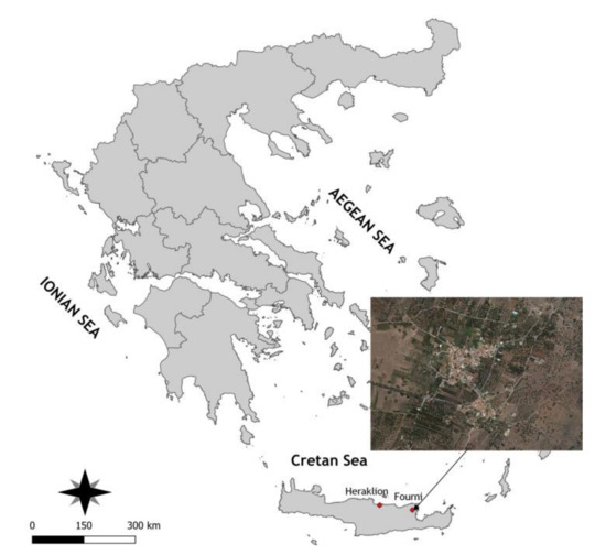
Figure 2.
Map of the study area with an overview of the settlement of Fourni in the island of Crete.
The settlement of Fourni belongs to the same climate zone with Heraklion, the largest city in Crete, in terms of their precipitation climate variability [76]. The village has suffered numerous flood events in the recent past, which caused significant damages to human properties, monuments and crops. Significant flood events in the area have been noticed at the end of the 20th century, at the beginning of the 90 s, while flood events are also quite frequent and intense during the last five years. In the settlement of Fourni there is no stormwater network, while there exist several flood storages at the boundaries of the village. The settlement does not have a separate sewer system, while sewerage needs are currently covered by the use of septic tanks.
The settlement of Fourni is considered an ungauged site for constructing IDF curves, because there are no short-duration rainfall observations available in the area. There exists an old rain gauge station installed in the village, however measurements from this instrument are only available on a monthly scale. Therefore, the data available for the study site of Fourni consist of 63 years (1949–2012) of monthly measurements, obtained from the database of the Prefecture of Crete. The age of the instrument can be denoted by the fact that there exist monthly rainfall measurements from the year 1932, with a gap during the period 1941–1948. Table 1 presents descriptive statistics for annual rainfall, as well as for annual rainfall monthly maxima at the study site of Fourni for the period 1949–2012. For the station of Heraklion, there exist short-duration rainfall measurements for quite a short period of 15 years, made available from the National Meteorological Service of Greece. The available data are annual maximum rainfall intensities and depths for time periods of 5 min, 10 min, 15 min, 30 min, 1 h, 2 h, 6 h, 12 h and 24 h. Monthly rainfall data at the rain gauge station of Heraklion have been also made available from the database of the Prefecture of Crete for a period of 37 years (1975–2011).

Table 1.
Descriptive statistics for annual rainfall and for annual rainfall monthly maxima at the study site of Fourni during the period 1949–2012.
The settlement of Fourni has quite a complex topographic relief, characterised by high slopes in certain parts of the settlement and a number of green spaces. For the purposes of the present work, the settlement of Fourni was mapped using topographic instruments, resulting in a detailed Digital Terrain Model (DTM) with elevations ranging in the interval from 306 m to 342 m. Elevations were measured at critical points of the village, namely at street junctions, at locations of flood storages and existing drainage infrastructure, as well as every 50 m along the two central streets of the settlement (see Section 4.3), where the main conduits of the stormwater network are located.
4. Results and Discussion
4.1. Nonstationary Analysis of Long-Duration Rainfall Maxima
Annual rainfall monthly maxima available for the study site of Fourni covering a period of 63 years (1949–2012) have been processed using a moving time window of 30-years length for fitting the GEV (and the Gumbel) distribution function and extracting return level estimates corresponding to return periods of 2, 5, 10, 20, 50, 100 and 200 years (see Section 2.1). The GEV/Gumbel distribution was fitted to all time windows and the extracted parameters and associated return level estimates were assumed to correspond to the last year of each such period, therefore covering the interval 1979–2012. The goodness of fit of the GEV/Gumbel distribution function was assessed using the Kolmogorov-Smirnov test and representative diagnostic plots, among several candidate distributions, that is, the Gamma, the Log-Normal, and so forth. The extracted GEV parameters (μ, σ, ξ) (or (μ, σ) for the Gumbel) from all the 30-years moving windows are presented in Figure 3 as a function of time in the studied interval 1979–2012. The ordinary least squares method has been used to fit linear and polynomial trends to all GEV/Gumbel parameters, to examine their variability in the studied period. The statistical significance of all trends has been judged using the t-test [60]. An analysis of variance (ANOVA), as well as the AIC and the BIC (see Section 2.1) of all statistically significant (at a 5% significance level) fitted models were then computed to identify the simplest trend in each parameter. Figure 3 includes the fitted statistically significant polynomial trends for both the GEV and the Gumbel parameters, as well as estimates of the AIC and BIC corresponding to these models.
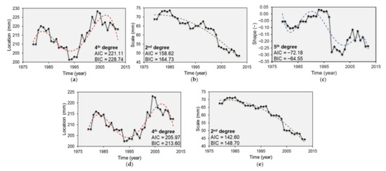
Figure 3.
Time-dependent estimates of GEV (a) location (mm); (b) scale (mm); (c) shape (−) parameters and Gumbel (d) location (mm); (e) scale (mm) parameters fitted to annual rainfall monthly maxima in Fourni, Crete. Red, green, and blue dashed lines represent statistically significant nonlinear trends for the location, scale and shape parameter of the extreme value distributions, respectively. The degree of the best-fitted polynomial trend and its AIC and BIC are included.
For all parameters of the GEV and the Gumbel distributions, statistically significant polynomial trends have been detected in the period 1979–2012. For the location and shape parameters the fitted polynomial trends are of order higher than three, identifying quite high variability in their estimates with time, with respect to the scale parameter. High variability observed especially in the shape parameter of the GEV distribution function, possibly affected by the medium size of moving time windows, is highly associated with varying intensity of most extreme rainfall events and is possibly attributed to variations of synoptic scale weather patterns. The location parameter, μ, for both the GEV and Gumbel distributions, is fitted by a polynomial of fourth order. This signifies distributions with lower means during the 90 s and higher mean values in the 21st century. The scale parameter, σ, of both distributions is fitted by a second order polynomial trend, identifying decreasing variance of extreme rainfall during the study period. The shape parameter, ξ, of the GEV is fitted by a fifth order polynomial trend, revealing significantly lighter tails in the period after 1995. The latter parameter, which dictates the limiting behaviour of the GEV, inclines towards increased variability of the respective rainfall return levels in the studied interval. However, it should be noted that rainfall extremes are usually better described by heavy-tailed distributions. Therefore, the shape parameter of the GEV, which is in fact the most uncertain parameter to estimate, depending critically on the sample size, is usually associated with positive values to describe rainfall extremes [77]. In the area under study and for annual rainfall monthly maxima the maximum likelihood estimates of the shape parameter were assessed to take negative values in a large part of the studied interval. These estimates were also verified using the method of L-moments. Nevertheless, no highly negative shape parameter estimates were detected. Interviewing residents in the study area resulted in verifying a significantly lower number of storm events in the last 15 years of the studied interval, as well as very few flooding events (this is not true for the period from 2017 to date, associated with more frequent and more intense storm events resulting in flooding and damages to property). Therefore, it was decided to retain the locally estimated values of the shape parameter, and not restrict it to a defined interval to comply with distribution functions with heavier tails.
Figure 4 presents time-dependent return level estimates for annual rainfall monthly maxima corresponding to return periods of 50 and 100 years for the GEV and Gumbel distribution functions in the period 1979–2012. Dashed lines correspond to maximum likelihood estimates, while colored areas represent 95% confidence intervals. Confidence intervals were assessed using the delta method [55]. For the GEV distribution function it is quite evident that there is a significant decrease of rainfall extremes after 1995, associated also with reduced uncertainty in return level estimates. The decrease observed reaches 27% for a return period of 50 years and 31% for a return period of 100 years. As for the period 1979–1995, a progressive increase in rainfall extremes can be observed. For the Gumbel distribution a decreasing trend for the entire series is evident with lowest values observed at the end of the study period. Differences in rainfall return level estimates reach 22% for a return period of 50 years, and 20% for a return period of 100 years. However, a slight increase in return level estimates can be spotted in the first decade of the study period.
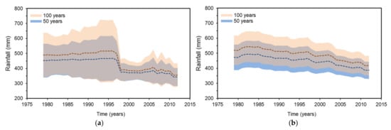
Figure 4.
Time-dependent estimates of 50-year and 100-year extreme monthly rainfall in Fourni, Crete, extracted by fitting: (a) a nonstationary GEV distribution function; (b) a nonstationary Gumbel distribution function. Dashed lines represent maximum likelihood estimates, while light blue and pink areas correspond to 95% confidence intervals for a return period of 50 and 100 years, respectively.
4.2. Rainfall Scaling and Construction of IDF Curves at the Ungauged Site
The construction of IDF curves for the study site of Fourni is obstructed by the lack of short-duration rainfall observations, necessary to estimate the relationship between rainfall intensity, duration and return period at short time scales. Short-duration rainfall extremes, determined by complex processes that can significantly alter under climate change conditions, can cause serious damage to human societies and properties through rapidly developing flash floods. To aid the construction of IDF curves at the study site of Fourni, available information on rainfall extremes in Heraklion is used in the present work. The wider area where Fourni is located presents quite similar statistical properties (especially in terms of standard deviation, coefficient of variation and skewness) of monthly rainfall and of annual daily maxima with the site of Heraklion [76]. Examining annual rainfall monthly maxima available for both sites for the period 1975–2011, maximum values of rainfall correspond to the same month in almost each year, while the correlation coefficient of the two series of annual maxima is high enough (Pearson’s correlation r = 0.61, Spearman’s correlation rs = 0.63). When fitting the GEV distribution function to both series of annual monthly maxima and estimating different quantiles of the series, it has been noted that the quantile ratio among the different quantiles is almost constant (ranges in the interval from 1.51 to 1.57). To further examine homogeneity of annual rainfall monthly maxima of the sites of Heraklion and Fourni, the bootstrap Anderson-Darling [78] and the Durbin and Knott [79] tests are also used, resulting in acceptance of the null hypothesis.
For the study site of Heraklion, where rainfall annual maxima of different durations are available, the GEV distribution function is first fitted to all available series of maxima. Equation (9) is used to describe IDF curves at the study site with a(T) and b(T) represented by Equations (11) and (12), respectively. Considering θ = 0 in Equation (12) for the sake of simplicity, the coefficients η, K and c are assessed through least squares fitting using Equations (13) and (14). Figure 5 presents IDF and DDF (Depth-Duration-Frequency) curves for the study site of Heraklion for return periods of 2, 5, 10, 20, 50, 100 and 200 years. Formulas extracted to estimate rainfall intensity, i, and depth, P, as a function of the rainfall duration, d, and return period, T, are also included.
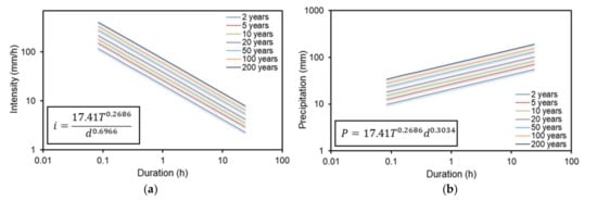
Figure 5.
(a) IDF and (b) DDF curves at the site of Heraklion, Crete, for return periods 2, 5, 10, 20, 50, 100 and 200 years.
Simple scaling presented in Section 2.2 is then implemented to rainfall return level estimates for different return periods (2, 5, 10, 20, 50, 100 and 200 years) and durations (5 min, 10 min, 30 min, 1 h, 2 h, 6 h, 12 h, 24 h and 1 month) for the study site of Heraklion. The hypothesis of scale invariance is applied here considering that annual maximum rainfall return levels will satisfy the scaling relationship of Equation (7). Least squares analysis is applied and self-similarity indices, β, are estimated for each one of the aforementioned return periods, as the slope of the linear regression relationship between the log-transformed values of the quantiles and the scale factors. Figure 6 presents the linear relationships between the log-transformed quantiles (log-transformed return levels) of rainfall intensity and log-transformed scale factors of different durations, for return periods of 2, 5, 10, 20, 50, 100 and 200 years. Estimates of the self-similarity index (estimates of −β) for the different return periods examined are also included in Figure 6. The self-similarity indices for the study site of Heraklion are estimated in the interval [0.685, 0.711] for return periods between 2 and 200 years. It should be noted that the abovementioned procedure was first implemented for rainfall durations up to 1 day (24 h) and self-similarity indices were assessed. The resulting values of the parameter β were estimated really close to the ones shown in Figure 6. The duration of one month was added to the diagram to aid the scaling of the rainfall maxima at the study site of Fourni, where only annual monthly maxima are available. Monthly maxima at the study site of Heraklion seem to be slightly overestimated by the fitted scaling law. However, it should be noted that due to the limited number of years of available monthly rainfall data at the site of Heraklion (37 years, 1975–2011), rainfall return level estimates for the different return periods, result from fitting a stationary GEV model. Due to high correlation of annual maximum rainfall observed between the study sites of Heraklion and Fourni, it can be noted that the assumption of stationarity underestimates the maximum rainfall quantiles for the studied 37 years (see results of the nonstationary analysis of annual rainfall monthly maxima for the study site of Fourni in Section 4.1), resulting when fitting a nonstationary model to the series of annual rainfall monthly maxima.
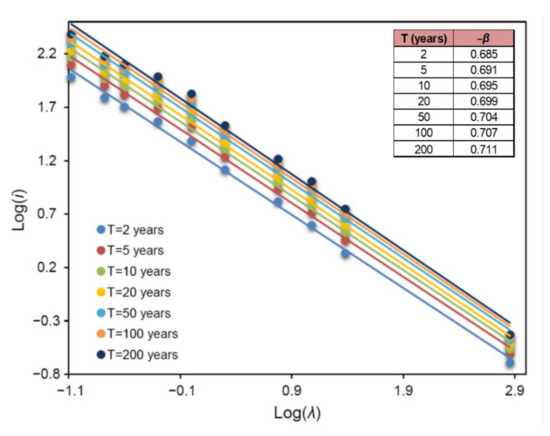
Figure 6.
Simple scaling of rainfall return level estimates for return periods 2, 5, 10, 20, 50, 100 and 200 years in Heraklion, Crete. Self-similarity indices, −β, for each return period are included.
The scaling model of Equation (7) was applied to time-dependent annual rainfall monthly maxima at the site of Fourni (see Section 4.1) using the self-similarity indices for the site of Heraklion, which is considered to belong to the same climatic zone in terms of extreme rainfall climate with the site of Fourni. Therefore, extreme rainfall of longer duration is temporally downscaled to shorter-duration amounts based on using the scaling properties of the process (described in Section 2.2) for each year in the interval 1979–2012. Figure 7 presents return level estimates of annual rainfall monthly maxima at the site of Fourni for different return periods and for four different rainfall durations, namely 10 min, 1 h, 6 h and 1 day in the study interval 1979–2021. The estimates were produced using the GEV distribution function, considering the adjusted trends in the parameters of the distribution for reasons of clarity (see Figure 3). For all four durations, the pattern of rainfall return level variation is quite similar. Rainfall return levels increase in the first almost 15 years of the study period and decrease afterwards, with lowest values observed at the end of the study period. Differences in extreme quantiles seem to be larger for higher durations. For all durations differences in rainfall quantiles in the interval 1979–2012 are estimated at almost 8.5%, 15%, 21%, 26.5%, 33%, 37% and 41% for return periods 2, 5, 10, 20, 50, 100 and 200 years, respectively.
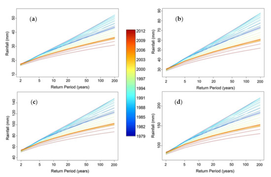
Figure 7.
Return level estimates of annual rainfall monthly maxima in Fourni for different return periods and for four different rainfall durations: (a) 10 min; (b) 1 h; (c) 6 h; (d) 1 day in the interval 1979–2012. Extracted rainfall estimates were produced including the adjusted trends in the GEV distribution parameters.
After estimating rainfall return levels of durations 5 min, 10 min, 30 min, 1 h, 2 h, 6 h, 12 h and 24 h from monthly quantiles corresponding to return periods of 2, 5,10, 20, 50, 100 and 200 years, IDF and DDF curves can be constructed for the study site of Fourni for each study year, applying the procedure described in Section 2.3. Equation (9) is again used to describe IDF curves at the study site with a(T) and b(T) represented by Equations (11) and (12), respectively. Considering θ = 0 in Equation (12), the coefficients η, K and c are assessed through least squares fitting using Equations (13) and (14). Figure 8 includes IDF and DDF curves at the site of Fourni for the year 1994, where the 95th percentile of the shape parameter, ξ(t), was assessed. The shape parameter was selected as a reference for determining extreme rainfall quantiles in longer time scales, due to its dominant role in defining the limiting behaviour of the modelled extremes. Therefore, a high enough percentile of the parameter was selected to be used in the subsequent construction of IDF curves, noticing also that the defined percentile corresponds to a non-negative value of the shape parameter. Figure 8 also includes the extracted formulas for the IDF and DDF curves at the site of Fourni. Comparing expressions of IDF and DDF curves extracted for the study sites of Heraklion and Fourni, the coefficient K of Equation (11) appears significantly increased in the latter, while the coefficient c is reduced. The coefficient η of Equation (12) does not differ significantly for both locations, mainly attributed to the approach used to temporally downscale rainfall intensity at the study site. Increases in a(T) of Equation (9) for the study site of Fourni, result in larger rainfall return level estimates compared to the site of Heraklion, a finding easily confirmed considering differences in altitude of the two sites.
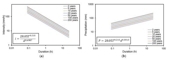
Figure 8.
(a) IDF and (b) DDF curves at the site of Fourni, Crete, for return periods 2, 5, 10, 20, 50, 100 and 200 years.
To estimate differences resulting from using a nonstationary moving window model for annual rainfall monthly maxima to the resulting rainfall quantiles used in the design process, a stationary GEV model was also fitted to the data and the scaling procedure was repeated. Table 2 summarises results of rainfall depth and intensity maximum likelihood return level estimates for return periods of 20, 50, 100 and 200 years at the study site of Fourni for rainfall durations of 10 min, 1 h and 24 h. The table compares estimates of rainfall depth and intensity estimated from applying a stationary GEV model to annual rainfall monthly maxima with those extracted using the nonstationary GEV distribution described in Section 2.1 and selecting the year corresponding to the 95th percentile of the shape parameter to construct the respective IDF and DDF curves. The nonstationary GEV model results in higher return level estimates for both the rainfall depth and intensity for all rainfall durations and return periods. Differences range from 7.5% for return periods of 20 years up to almost 20.5% for return periods of 200 years. For a return period of 100 years, the differences in rainfall quantiles exceed 16%.
Table 2.
Rainfall depth and intensity maximum likelihood return level estimates in Fourni, for return periods of 20, 50, 100 and 200 years and rainfall durations of 10 min, 1 h and 24 h, extracted by fitting the stationary and a nonstationary (95th percentile of ξ) GEV distribution to annual rainfall monthly maxima.
Table 3 presents results of rainfall depth and intensity corresponding to the upper 97.5% confidence interval of return level estimates (see Figure 4) for return periods of 20, 50, 100 and 200 years at the study site of Fourni for rainfall durations of 10 min, 1 h and 24 h. As in Table 2 and Table 3 compares estimates of rainfall depth and intensity estimated from applying a stationary GEV model to annual rainfall monthly maxima with those extracted using the nonstationary GEV distribution described in Section 2.1 and selecting the year corresponding to the 95th percentile of the shape parameter. The respective differences range from more than 19.5% for a return period of 20 years to over 50% for a return period of 200 years.
Table 3.
Rainfall depth and intensity upper 97.5% return level estimates in Fourni, for return periods of 20, 50, 100 and 200 years and rainfall durations of 10 min, 1 h and 24 h, extracted by fitting the stationary and a nonstationary (95th percentile of ξ) GEV distribution to annual rainfall monthly maxima.
4.3. Design of a Stormwater Network in a Changing Climate
In this study a new stormwater network was designed for the study site of Fourni using the SWMM software (see Section 2.4). The design rainfall used to force the stormwater network corresponds to a return period of 100 years and a duration of 10 min and was assessed using the approach described in Section 2.1 and Section 2.2, assuming a nonstationary extreme rainfall climate. A DTM constructed for the purposes of this research enabled the preliminary design of the systems’ conduits with slopes mainly following those of the terrain, while available flood storages in the study area defined the system’s outlets. Eliminating overflows of the system’s manholes was a major criterion used in the design process followed, together with other constraints described in Section 2.4. It should be noted that under such extreme conditions, a maximum ratio of flow depth to the diameter of the conduit is quite difficult to be preserved for the entire network. Therefore, especially for the primary conduits of the network (main conduits along the central streets of the village), elimination of overflow volumes was used as a major criterion in the design process.
More specifically, the stormwater network of Fourni was designed with a total of 100 circular PVC conduits and 55 manholes mainly located at intersections of conduits or at major bends. The designed stormwater network operates with two main conduits located along the two central streets of the settlement and other smaller conduits covering the entire study area. The stormwater network has five outlets (OUT1 to OUT5) to existing infrastructure, namely, one (OUT1) leading to an open channel at the southwestern part of the settlement, three (OUT2, OUT3, OUT5) leading to existing flood storages at the southwestern and northwestern parts, and one (OUT4) ending at an existing old drainage pipe at the northwestern part of Fourni, collecting water and transferring it away from the study area and into the fields. Two other flood storages are also available at the southeastern part of the settlement; however, the topography of the village did not allow to include them in the design of the network. Figure 9 presents a schematic diagram (overview) of the designed stormwater network with its conduits and manholes (Figure 9a), as well as its five outlets (Figure 9b).
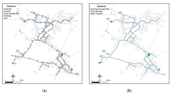
Figure 9.
Overview of the designed stormwater network in Fourni with (a) conduits and manholes and available flood storages; (b) five outlets of the network.
The study of inflows and throughflows into the designed system’s conduits and manholes was performed using SWMM model (Section 2.4). SWMM is a commonly used software combining both hydrologic and hydraulic analysis of stormwater networks, providing accurate modelling of sewer systems’ elements including modelling of backwater effects and reverse flow. The land surface of the settlement was first divided into subcatchments, each draining to a specific discharge point. Catchment delineation was performed based on terrain topography, with larger subcatchments corresponding to green spaces draining at the two central conduits of the network. Rainfall-runoff analysis required several subcatchment parameters, including area, slope, imperviousness and infiltration for different areas. The imperviousness parameter of the subcatchments was set at 25%. The total surface runoff of the study area was assessed at around 11.5 m3/s. The infiltration model used for subcatchments in the present work was the one based on Curve Number, while the conductivity coefficient used for green spaces was considered equal to 0.035. For the system’s conduits the minimum slope was considered equal to 0.10% and the minimum diameter was set to DN 400 following the Greek standards. Hydraulic analysis of the network was performed using the dynamic wave routing model. The normal flow criterion was based on the flow’s free surface slope and the Froude number of the flow. The Manning’s roughness coefficient of conduits was set at 0.011 [73]. A 10 min simulation time step was selected for both the hydrologic and hydraulic routing computations.
Figure 10 and Figure 11 present an overview of the estimated diameters for the designed system’s conduits. Figure 10 presents results of the analysis when nonstationarity of the rainfall climate is not considered (see Section 4.2). In this case a stationary GEV distribution function was fitted to annual rainfall monthly maxima at the site of Fourni and the assessed quantiles were then scaled to shorter durations following the procedure analysed in Section 2.2. Figure 11 presents conduit diameters for the studied stormwater network in Fourni under a changing climate (implementing 30-year moving time windows to annual rainfall monthly maxima and selecting return level estimates of the year corresponding to the 95th percentile of the estimated GEV shape parameter to be used in the scaling process). A comparative analysis performed for the two cases, identifies increased diameters of conduits for the second case. More specifically, under the assumption of stationarity, the system’s diameters range from DN 400 to DN 600, while when nonstationarity of annual monthly rainfall maxima is considered, the upper bound of the range of conduit diameters increases to DN 800. More specifically, in the latter case the carrying capacity of the central conduits of the system need to increase significantly. Conduits of diameter DN 600 are replaced with respective ones of diameter DN 800, while others of diameter DN 500 change to DN 600. Secondary conduits of diameter DN 400 remain mostly unchanged.
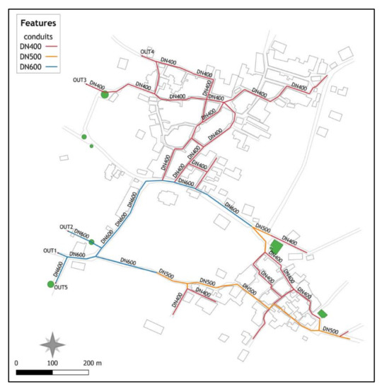
Figure 10.
Overview of assessed diameters of stormwater network’s conduits in Fourni considering stationarity of annual rainfall monthly maxima.
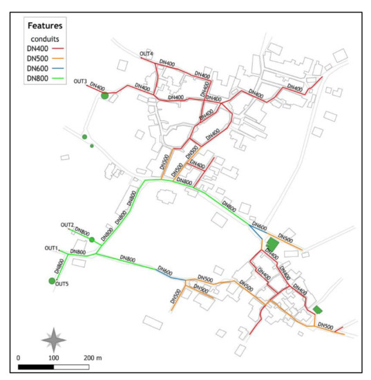
Figure 11.
Overview of assessed diameters of stormwater network’s conduits in Fourni considering nonstationarity of annual rainfall monthly maxima.
5. Conclusions
The present work introduces a new and easy-to-apply approach to construct IDF curves at a site with no short-duration rainfall observations (ungauged site) under the assumption of a changing climate. The IDF curves constructed are then utilised in the design of a stormwater network following the Greek standards. The proposed methodology to derive IDF curves uses information on rainfall dynamics from a site with relatively homogeneous extreme rainfall climate with the study site, and produces inferences based on the hypothesis of scale invariance of the annual maximum rainfall intensity.
The fact that IDF curves are currently constructed based on the assumption of stationarity, neglecting climate variability and climate change can lead to significantly biased estimates of rainfall return levels for return periods used in the design of urban infrastructure. The existing strong evidence of a changing climate, expected to alter the intensity, the duration, and the probability (frequency) of occurrence of extreme precipitation events, emphasizes the need for a nonstationary analysis of such events to produce more reliable and robust estimates for extreme rainfall. The proposed approach considers nonstationarity in annual rainfall monthly maxima at the study site, significantly affecting the construction of IDF curves, as well as results of hydrologic and hydraulic design, altering the diameters of stormwater network conduits and therefore modifying the hydraulic bearing capacity of the network. It is therefore noted that the assumption of a stationary climate should be abandoned today, highly prioritizing the need for climate variability to be considered.
The proposed approach was implemented at the study site of Fourni in Crete, using available information on rainfall dynamics from the site of Heraklion, which is considered relatively homogeneous in terms of extreme rainfall with the study site. IDF curves constructed for the site of Heraklion have been validated against rainfall return level estimates extracted directly from fitting the stationary GEV distribution to observed annual rainfall maxima of sub-hourly to daily durations, as well as against rainfall quantiles from existing reports of the Greek Ministry of Environment and Energy. A nonstationary GEV distribution function was fitted to annual rainfall monthly maxima in Fourni, using a moving 30-year time window and a sufficiently high quantile of the shape parameter was selected to define rainfall monthly return levels. The latter were combined with a scaling approach to produce short-duration rainfall return levels and construct IDF curves. The aforementioned approach, which considers nonstationarity in annual rainfall monthly maxima, resulted in increased estimates of rainfall return levels up to 20.5%. A newly designed stormwater network at the site of Fourni based on the assumption of a nonstationary climate is characterised by increased diameters of its primary conduits, compared to the ones resulting under fully stationary conditions.
Author Contributions
Conceptualization, P.G. and C.I.; methodology, P.G. and C.I.; software, P.G. and C.I.; validation, P.G.; formal analysis, P.G. and C.I.; investigation, C.I.; resources, P.G. and C.I.; data curation, C.I.; writing—original draft preparation, P.G.; writing—review and editing, P.G. and C.I.; visualization, P.G. and C.I.; supervision, P.G.; project administration, P.G. All authors have read and agreed to the published version of the manuscript.
Funding
This research received no external funding.
Institutional Review Board Statement
Not applicable.
Informed Consent Statement
Not applicable.
Data Availability Statement
Meteorological data of the present work was provided by the Greek National Meteorological Service and the Prefecture of Crete, Greece.
Conflicts of Interest
The authors declare no conflict of interest.
References
- Norbiato, D.; Borga, M.; Sangati, M.; Zanon, F. Regional frequency analysis of extreme precipitation in the eastern Italian Alps and the 29 August 2003 flash flood. J. Hydrol. 2007, 345, 149–166. [Google Scholar] [CrossRef]
- Morita, M. Flood risk analysis for determining optimal flood protection levels in urban river management. J. Flood Risk Manag. 2008, 1, 142–149. [Google Scholar] [CrossRef]
- Fontanazza, C.M.; Freni, G.; La Loggia, G.; Notaro, V. Uncertainty evaluation of design rainfall for urban flood risk analysis. Water Sci. Technol. 2011, 63, 2641–2650. [Google Scholar] [CrossRef] [PubMed]
- Zhou, Q.; Mikkelsen, P.S.; Halsnæs, K.; Arnbjerg-Nielsen, K. Framework for economic pluvial flood risk assessment considering climate change effects and adaptation benefits. J. Hydrol. 2012, 414, 539–549. [Google Scholar] [CrossRef]
- Cheng, L.; AghaKouchak, A. Nonstationary precipitation intensity-duration-frequency curves for infrastructure design in a changing climate. Sci. Rep. 2014, 4, 1–6. [Google Scholar] [CrossRef] [PubMed]
- Da Silva, C.V.F.; Schardong, A.; Garcia, J.I.B.; Oliveira, C.D.P.M. Climate change impacts and flood control measures for highly developed urban watersheds. Water 2018, 10, 829. [Google Scholar] [CrossRef]
- Yan, H.; Sun, N.; Wigmosta, M.; Skaggs, R.; Hou, Z.; Leung, L.R. Next-generation intensity–duration–frequency curves to reduce errors in peak flood design. J. Hydrol. Eng. 2019, 24, 04019020. [Google Scholar] [CrossRef]
- Yan, H.; Sun, N.; Wigmosta, M.; Leung, L.R.; Hou, Z.; Coleman, A.; Skaggs, R. Evaluating next-generation intensity–duration–frequency curves for design flood estimates in the snow-dominated western United States. Hydrol. Process. 2020, 34, 1255–1268. [Google Scholar] [CrossRef]
- Wallis, J.; Schaefer, M.; Baker, B.; Taylor, G. Regional precipitation-frequency analysis and spatial mapping for 24- and 2-h durations for Washington State. Hydrol. Earth Syst. Sci. Dis. 2007, 11, 415–442. [Google Scholar] [CrossRef]
- Renard, B.; Lall, U. Regional frequency analysis conditioned on large-scale atmospheric or ocean fields. Water Resour. Res. 2014, 50, 9536–9554. [Google Scholar] [CrossRef]
- Devkota, S.; Shakya, N.M.; Sudmeier-Rieux, K.; Jaboyedoff, M.; Van Westen, C.J.; Mcadoo, B.G.; Adhikari, A. Development of monsoonal rainfall intensity-duration-frequency (IDF) relationship and empirical model for data-scarce situations: The case of the Central-Western Hills (Panchase region) of Nepal. Hydrology 2018, 5, 27. [Google Scholar] [CrossRef]
- El-Sayed, E.A.H. Generation of rainfall intensity duration frequency curves for ungauged sites. Nile Basin Water Sci. Eng. J. 2011, 4, 112–124. [Google Scholar]
- Liew, S.C.; Raghavan, S.V.; Liong, S.Y. How to construct future IDF curves, under changing climate, for sites with scarce rainfall records? Hydrol. Process. 2014, 28, 3276–3287. [Google Scholar] [CrossRef]
- Rodriguez, R.D.; Singh, V.P.; Pruski, F.F.; Calegario, A.T. Using entropy theory to improve the definition of homogeneous regions in the semi-arid region of Brazil. Hydrol. Sci. J. 2016, 61, 2096–2109. [Google Scholar] [CrossRef]
- Ouali, D.; Chebana, F.; Ouarda, T.B. Non-linear canonical correlation analysis in regional frequency analysis. Stoch. Environ. Res. Risk Assess. 2016, 30, 449–462. [Google Scholar] [CrossRef]
- Pandey, G.R.; Nguyen, V.T.V. A comparative study of regression-based methods in regional flood frequency analysis. J. Hydrol. 1999, 225, 92–101. [Google Scholar] [CrossRef]
- Ouarda, T.B.; Cunderlik, J.M.; St-Hilaire, A.; Barbet, M.; Bruneau, P.; Bobée, B. Data-based comparison of seasonality-based regional flood frequency methods. J. Hydrol. 2006, 330, 329–339. [Google Scholar] [CrossRef]
- Cannon, A.J. An intercomparison of regional and at-site rainfall extreme value analyses in southern British Columbia, Canada. Can. J. Civ. Eng. 2015, 42, 107–119. [Google Scholar] [CrossRef]
- Ouali, D.; Chebana, F.; Ouarda, T.B. Fully nonlinear statistical and machine-learning approaches for hydrological frequency estimation at ungauged sites. J. Adv. Model. Earth Syst. 2017, 9, 1292–1306. [Google Scholar] [CrossRef]
- Ouali, D.; Chebana, F.; Ouarda, T.B. Quantile regression in regional frequency analysis: A better exploitation of the available information. J. Hydrometeorol. 2016, 17, 1869–1883. [Google Scholar] [CrossRef]
- Cannon, A.J. Quantile regression neural networks: Implementation in R and application to precipitation downscaling. Comput. Geosci. 2011, 37, 1277–1284. [Google Scholar] [CrossRef]
- Ouali, D.; Cannon, A.J. Estimation of rainfall intensity–duration–frequency curves at ungauged locations using quantile regression methods. Stoch. Environ. Res. Risk Assess. 2018, 32, 2821–2836. [Google Scholar] [CrossRef]
- Koutsoyiannis, D.; Kozonis, D.; Manetas, A. A mathematical framework for studying rainfall intensity-duration-frequency relationships. J. Hydrol. 1998, 206, 118–135. [Google Scholar] [CrossRef]
- Veneziano, D.; Furcolo, P. Multifractality of rainfall and scaling of intensity-duration-frequency curves. Water Resour. Res. 2002, 38, 42-1. [Google Scholar] [CrossRef]
- Singh, V.P.; Zhang, L. IDF curves using the Frank Archimedean copula. J. Hydrol. Eng. 2007, 12, 651–662. [Google Scholar] [CrossRef]
- Ganguli, P.; Coulibaly, P. Does nonstationarity in rainfall require nonstationary intensity–duration–frequency curves? Hydrol. Earth Syst. Sci. 2017, 21, 6461–6483. [Google Scholar] [CrossRef]
- Salas, J.D.; Obeysekera, J. Revisiting the concepts of return period and risk for nonstationary hydrologic extreme events. J. Hydrol. Eng. 2014, 19, 554–568. [Google Scholar] [CrossRef]
- Kharin, V.V.; Zwiers, F.W. Estimating extremes in transient climate change simulations. J. Clim. 2005, 18, 1156–1173. [Google Scholar] [CrossRef]
- El Adlouni, A.; Ouarda, T.B.M.; Zhang, X.; Roy, R.; Bobee, B. Generalized maximum likelihood estimators for the nonstationary generalized extreme value model. Water Resour. Res. 2007, 43, W03410. [Google Scholar] [CrossRef]
- Cooley, D. Extreme value analysis and the study of climate change. Clim. Change 2009, 97, 77–83. [Google Scholar] [CrossRef]
- Towler, E.; Rajagopalan, B.; Gilleland, E.; Summers, R.S.; Yates, D.; Katz, R.W. Modeling hydrologic and water quality extremes in a changing climate: A statistical approach based on extreme value theory. Water Resour. Res. 2010, 46, W11504. [Google Scholar] [CrossRef]
- Cheng, L.; AghaKouchak, A.; Gilleland, E.; Katz, R.W. Non-stationary extreme value analysis in a changing climate. Clim. Chang. 2014, 127, 353–369. [Google Scholar] [CrossRef]
- Sarhadi, A.; Soulis, E.D. Time-varying extreme rainfall intensity-duration-frequency curves in a changing climate. Geophys. Res. Lett. 2017, 44, 2454–2463. [Google Scholar] [CrossRef]
- Agilan, V.; Umamahesh, N.V. Modelling nonlinear trend for developing non-stationary rainfall intensity–duration–frequency curve. Int. J. Climatol. 2017, 37, 1265–1281. [Google Scholar] [CrossRef]
- Ouarda, T.B.; Charron, C. Nonstationary temperature-duration-frequency curves. Sci. Rep. 2018, 8, 1–8. [Google Scholar] [CrossRef]
- Silva, D.F.; Simonovic, S.P.; Schardong, A.; Goldenfum, J.A. Assessment of non-stationary IDF curves under a changing climate: Case study of different climatic zones in Canada. J. Hydrol. Reg. Stud. 2021, 36, 100870. [Google Scholar] [CrossRef]
- Yan, L.; Xiong, L.; Jiang, C.; Zhang, M.; Wang, D.; Xu, C.Y. Updating intensity–duration–frequency curves for urban infrastructure design under a changing environment. WIREs Water 2021, 8, e1519. [Google Scholar] [CrossRef]
- Nguyen, V.T.V.; Nguyen, T.D.; Wang, H. Regional estimation of short duration rainfall extremes. Water Sci. Technol. 1998, 37, 15–19. [Google Scholar] [CrossRef]
- Yu, P.S.; Yang, T.C.; Lin, C.S. Regional rainfall intensity formulas based on scaling property of rainfall. J. Hydrol. 2004, 295, 108–123. [Google Scholar] [CrossRef]
- Bougadis, J.; Adamowski, K. Scaling model of a rainfall intensity-duration-frequency relationship. Hydrol. Process. 2006, 20, 3747–3757. [Google Scholar] [CrossRef]
- Sun, Y.; Wendi, D.; Kim, D.E.; Liong, S.Y. Deriving intensity–duration–frequency (IDF) curves using downscaled in situ rainfall assimilated with remote sensing data. Geosci. Lett. 2019, 6, 1–12. [Google Scholar] [CrossRef]
- Burlando, P.; Rosso, R. Scaling and muitiscaling models of depth-duration-frequency curves for storm precipitation. J. Hydrol. 1996, 187, 45–64. [Google Scholar] [CrossRef]
- Langousis, A.; Carsteanu, A.A.; Deidda, R. A simple approximation to multifractal rainfall maxima using a generalized extreme value distribution model. Stoch. Environ. Res. Risk Assess. 2013, 27, 1525–1531. [Google Scholar] [CrossRef]
- Bara, M.; Gaal, L.; Kohnova, S.; Szolgay, J.; Hlavcova, K. On the use of the simple scaling of heavy rainfall in a regional estimation of IDF curves in Slovakia. J. Hydrol. Hydromech. 2010, 58, 49. [Google Scholar] [CrossRef]
- Ghanmi, H.; Bargaoui, Z.; Mallet, C. Estimation of intensity-duration-frequency relationships according to the property of scale invariance and regionalization analysis in a Mediterranean coastal area. J. Hydrol. 2016, 541, 38–49. [Google Scholar] [CrossRef]
- Yeo, M.H.; Nguyen, V.T.V.; Kpodonu, T.A. Characterizing extreme rainfalls and constructing confidence intervals for IDF curves using Scaling-GEV distribution model. Int. J. Climatol. 2021, 41, 456–468. [Google Scholar] [CrossRef]
- Willems, P.; Arnbjerg-Nielsen, K.; Olsson, J.; Nguyen, V.T.V. Climate change impact assessment on urban rainfall extremes and urban drainage: Methods and shortcomings. Atmos. Res. 2012, 103, 106–118. [Google Scholar] [CrossRef]
- Arnbjerg-Nielsen, K.; Willems, P.; Olsson, J.; Beecham, S.; Pathirana, A.; Bulow Gregersen, I.; Madsen, H.; Nguyen, V.T.V. Impacts of climate change on rainfall extremes and urban drainage systems: A review. Water Sci. Technol. 2013, 68, 16–28. [Google Scholar] [CrossRef]
- Langeveld, J.G.; Schilperoort, R.P.S.; Weijers, S.R. Climate change and urban wastewater infrastructure: There is more to explore. J. Hydrol. 2013, 476, 112–119. [Google Scholar] [CrossRef]
- Willems, P. Revision of urban drainage design rules after assessment of climate change impacts on precipitation extremes at Uccle, Belgium. J. Hydrol. 2013, 496, 166–177. [Google Scholar] [CrossRef]
- Moore, T.L.; Gulliver, J.S.; Stack, L.; Simpson, M.H. Stormwater management and climate change: Vulnerability and capacity for adaptation in urban and suburban contexts. Clim. Change 2016, 138, 491–504. [Google Scholar] [CrossRef]
- Kumar, S.; Agarwal, A.; Ganapathy, A.; Villuri, V.G.K.; Pasupuleti, S.; Kumar, D.; Kaushal, D.R.; Gosain, A.K.; Sivakumar, B. Impact of climate change on stormwater drainage in urban areas. Stoch. Hydrol. Hydraul. 2021, 36, 77–96. [Google Scholar] [CrossRef]
- Huq, E.; Abdul-Aziz, O.I. Climate and land cover change impacts on stormwater runoff in large-scale coastal-urban environments. Sci. Total Environ. 2021, 778, 146017. [Google Scholar] [CrossRef]
- Kourtis, I.M.; Tsihrintzis, V.A. Adaptation of urban drainage networks to climate change: A review. Sci. Total Environ. 2021, 771, 145431. [Google Scholar] [CrossRef] [PubMed]
- Coles, S. An Introduction to Statistical Modeling of Extreme Values; Springer: London, UK, 2001; p. 208. [Google Scholar]
- Galiatsatou, P.; Prinos, P. Modeling non-stationary extreme waves using a point process approach and wavelets. Stoch. Environ. Res. Risk Assess. 2011, 25, 165–183. [Google Scholar] [CrossRef]
- Hosking, J.R. L-moments: Analysis and estimation of distributions using linear combinations of order statistics. J. R. Stat. Soc. Ser. B (Methodol.) 1990, 52, 105–124. [Google Scholar] [CrossRef]
- Galiatsatou, P.; Prinos, P. Bivariate analysis of extreme wave and storm surge events. Determining the failure area of structures. Open Ocean Eng. J. 2011, 4, 3–14. [Google Scholar] [CrossRef][Green Version]
- Galiatsatou, P.; Makris, C.; Prinos, P.; Kokkinos, D. Nonstationary joint probability analysis of extreme marine variables to assess design water levels at the shoreline in a changing climate. Nat. Hazards 2019, 98, 1051–1089. [Google Scholar] [CrossRef]
- Galiatsatou, P.; Makris, C.; Krestenitis, Y.; Prinos, P. Nonstationary Extreme Value Analysis of Nearshore Sea-State Parameters under the Effects of Climate Change: Application to the Greek Coastal Zone and Port Structures. J. Mar. Sci. Eng. 2021, 9, 817. [Google Scholar] [CrossRef]
- Gupta, V.K.; Waymire, E. Multiscaling properties of spatial rainfall and river flow distributions. J. Geophys. Res. Atmos. 1990, 95, 1999–2009. [Google Scholar] [CrossRef]
- Veneziano, D.; Lepore, C.; Langousis, A.; Furcolo, P. Marginal methods of intensity-duration-frequency estimation in scaling and nonscaling rainfall. Water Resour. Res. 2007, 43. [Google Scholar] [CrossRef]
- Innocenti, S.; Mailhot, A.; Frigon, A. Simple scaling of extreme precipitation in North America. Hydrol. Earth Syst. Sci. 2017, 21, 5823–5846. [Google Scholar] [CrossRef]
- Van de Vyver, H. Bayesian estimation of rainfall intensity–duration–frequency relationships. J. Hydrol. 2015, 529, 1451–1463. [Google Scholar] [CrossRef]
- Raudkivi, A.J. Hydrology: An Advanced Introduction to Hydrological Processes and Modelling; Pergamon Press: New York, NY, USA, 1979. [Google Scholar]
- Chow, V.T. Handbook of Applied Hydrology; McGraw-Hill Book: New York, NY, USA, 1988. [Google Scholar]
- Singh, V.P. Elementary Hydrology; Prentice Hall: Englewood Cliffs, NJ, USA, 1992. [Google Scholar]
- Shaw, E.M.; Beven, K.J.; Chappell, N.A.; Lamb, R. Hydrology in Practice; CRC Press: Boca Raton, FL, USA, 2010. [Google Scholar]
- Chen, C. Rainfall Intensity-Duration-Frequency Formulas. J. Hydraul. Eng. 1983, 109, 1603–1621. [Google Scholar] [CrossRef]
- Koutsoyiannis, D. Statistical Hydrology; National Technical University: Athens, Greek, 1997. [Google Scholar] [CrossRef]
- James, W.; Huber, W.C.; Dickinson, R.E.; Pitt, R.E.; James, W.R.C.; Roesner, L.A.; Aldrich, J.A. User’s Guide to SWMM5-CHI Publications, 13th ed.; CHI Water: Guelph, ON, Canada, 2011. [Google Scholar]
- Rossman, L.A. Storm Water Management Model User’s Manual Version 5.1; United States Environmental Protection Agency (USEPA): Cincinnati, OH, USA, 2015. [Google Scholar]
- Rossman, L.A.; Huber, W.C. Storm Water Management Model Reference Manual Volume I—Hydrology (Revised); EPA/600/R-15/162A; National Risk Management Laboratory Office of Research and Development; United States Environmental Protection Agency (USEPA): Cincinnati, OH, USA, 2016. [Google Scholar]
- Niazi, M.; Nietch, C.; Maghrebi, M.; Jackson, N.; Bennett, B.R.; Tryby, M.; Massoudieh, A. Storm water management model: Performance review and gap analysis. J. Sustain. Water Built. Environ. 2017, 3, 04017002. [Google Scholar] [CrossRef] [PubMed]
- Shao, Z.; Zhang, X.; Li, S.; Deng, S.; Chai, H. A novel SWMM based algorithm application to storm sewer network design. Water 2017, 9, 747. [Google Scholar] [CrossRef]
- Markonis, Y.; Batelis, S.C.; Dimakos, Y.; Moschou, E.; Koutsoyiannis, D. Temporal and spatial variability of rainfall over Greece. Theor. Appl. Climatol. 2017, 130, 217–232. [Google Scholar] [CrossRef]
- Serinaldi, F.; Kilsby, C.G. Rainfall extremes: Toward reconciliation after the battle of distributions. Water Resour. Res. 2014, 50, 336–352. [Google Scholar] [CrossRef]
- Scholz, F.W.; Stephens, M.A. K-sample Anderson–Darling tests. J. Am. Stat. Assoc. 1987, 82, 918–924. [Google Scholar]
- Durbin, J.; Knott, M. Components of Cramér–von Mises statistics. I. J. R. Stat. Soc. Ser. B (Methodol.) 1972, 34, 290–307. [Google Scholar] [CrossRef]


Publisher’s Note: MDPI stays neutral with regard to jurisdictional claims in published maps and institutional affiliations. |
© 2022 by the authors. Licensee MDPI, Basel, Switzerland. This article is an open access article distributed under the terms and conditions of the Creative Commons Attribution (CC BY) license (https://creativecommons.org/licenses/by/4.0/).