Abstract
Agricultural irrigation consumes about 70% of freshwater globally every year. To improve the water-use efficiency in agricultural irrigation is critical as we move toward water sustainability. An irrigation scheduler determines how much water to irrigate and when to irrigate for an agricultural field. To get a high-resolution irrigation-scheduling solution for a large-scale agricultural field is still an open research problem. In this work, we propose a knowledge-based optimal irrigation-scheduling approach for large-scale agricultural fields that are equipped with center pivot irrigation systems. The proposed scheduler is designed in the framework of model predictive control. The objective of the proposed scheduler is to maximize crop yield while minimizing irrigation water consumption and the associated electricity usage. First, we introduce a structure-preserving model reduction technique to significantly reduce the dimensionality of agro-hydrological systems. Then, based on the reduced model, an optimization-based scheduler is designed. In the design of the scheduler, knowledge from farmers is taken into account to further reduce the computational complexity of the scheduler. The proposed approach explicitly considers both the irrigation time and the irrigation amount as decision variables to keep the crop within the stress-free zone considering the weather uncertainty and heterogeneous soil types for large agricultural fields. The proposed approach is applied to three different scenarios with different soil types, crops, and weather uncertainty. The results show that in all the conditions, the scheduler is capable of keeping the crops stress-free, which results in maximum yield and, at the same time, minimizes water consumption and irrigation events.
1. Introduction
Freshwater scarcity is one of the most critical global risks the world is currently facing [1] due mainly to population growth, climate change, and environmental pollution. Almost 70% of the total freshwater [2] is consumed in agricultural irrigation every year. Moreover, the efficacy of the current irrigation methods is around 50% to 60% [3], which is not adequate to save water usage significantly. Therefore, to alleviate water-usage efficiency is a very important measure for feeding the growing population and managing the water crisis.
The common irrigation practice includes open-loop control, which means no real-time information from the farm is used for the irrigation decision. Moreover, it mostly depends on the farmer’s observation and experience about the farm instead of actual field conditions such as soil moisture and weather conditions, which may lead to excessive or insufficient irrigation. One of the solutions to handle the issue is closed-loop irrigation, where real-time information from the field is utilized to make irrigation decisions. There are different control strategies based on real-time field feedback that have been mentioned in the literature. A modified proportional-integral-derivative (PID) controller is designed for excellent regulation of soil moisture that responds to changes in environmental conditions quickly [4]. Model predictive control (MPC) has gained increasing interest and attention in the literature in the past number of years as an optimal feedback-control method. McCarthy et al. developed a MPC using crop production models to optimize soil moisture and irrigation time [5]. Similarly, a MPC was designed by Delgoda et al. to minimize root zone soil moisture deficit and the irrigation amount with a limit on water supply [6]. In the same line of research, a zone MPC algorithm was proposed to maintain soil moisture within a target zone instead of a set-point control, which shows further water conservation. These types of irrigation-control methods mainly emphasis short periods for a couple of minutes or an hour of irrigation management. All these studies have one common objective to maintain the soil moisture deficit for a fixed set point or predetermined zone.
Irrigation scheduling is well-defined planning for agriculture irrigation management that determines the irrigation amount and the appropriate irrigation time for a much longer period, such as the entire harvesting crop season. The scheduler typically considers the field soil moisture content, plant water consumption, evapotranspiration (ET), and historical weather and climate information to make the irrigation prescriptions [7,8,9]. To maximize crop yield, a dynamic-programming (DP) algorithm is developed to provide optimal irrigation allocation using conditional soil-moisture probability distributions and ET in a stochastic control framework [10]. To maximize potential crop production through appropriate water allocation, quadratic programming (QP) optimization is designed based on real-time evaluations of crop water requirements [11]. For maximum yield and uniform irrigation allocation, a genetic algorithm (GA) was designed by Hassan et al. to provide an optimal irrigation amount based on crop parameters and crop stress factors using remote-sensing images [12]. Irrespective of the objectives, in the aforementioned studies, the scheduler provides the irrigation decisions at the starting of the crop growing season, and the solution does not change based on weather uncertainty or other field conditions.
Recently, Nahar et al. proposed a hierarchical closed-loop approach to provide the optimal irrigation amount for both long and short time periods based on a one-dimensional linear-parameter-varying (LPV) model [13]. The top-level scheduler provides the set-points for the low-level controller considering the crop yield and water consumption, and the low-level controller follows the soil moisture set-points. In [14], Kassing et al. proposed a two-level optimization method to solve an optimal irrigation problem of a large-scale plantation for both seasonal and daily scales based on the Aquacrop-OS model. The scheduler decides the optimal irrigation amount for the whole season to maximize crop yield, while the MPC is designed for the daily scale, considering the decision from the top-level scheduler, daily operational constraints, and weather forecast. To handle the nonlinearity of the system, ref. [15] proposed a scheduling approach based on a data-driven model in the framework of MPC with discrete decision variables for one-dimensional agro-hydrological systems. One common feature of the above scheduling studies is that the scheduler and controller are designed using a simplified linear model that considers a one-dimensional flow regime approach.
The three-dimensional model is necessary for precision irrigation because it can capture the runoff, horizontal flows in the presence of slopes, and different soil types. An agrohydrological system can be modeled by a three-dimensional Richards equation, which is a partial differential equation (PDE) in nature. The finer discretization is required not only to ensure the numerical stability but also to ensure the local equilibrium between the soil water content and the soil water potential [16]. The finer discretization produces a very high number of nodes; therefore, it increases the number of states of the discretized agricultural field as high as (10–10). The direct application of the state-space model (12) is computationally challenging for the optimization step in the MPC solving if states are the decision variables or the state constraints present. For example, there are three direct approaches to solve numerically the MPC optimization problem: single shooting, multiple shooting, and collocation. For nonlinear systems, multiple shooting and collocation-based approaches are more preferred because of the faster convergence and better numerical stability. However, the states of the system become the decision variables in both approaches. So, for a large-scale system like an agro-hydrological system, the optimization problem may become intractable. Similarly, in Zone MPC, the presence of slack variables (twice the size of the states) as the decision variables and the state constraints make the optimization problem a computationally dominant task.
Model reduction is one of the efficient techniques to handle the problem by reducing the dimension of states. Therefore, the number of decision variables and the number of state constraints decrease to a huge extent. A few popular classical model-reduction techniques are proper orthogonal decomposition (POD), optimal Hankel norm reduction, balanced truncation methods [17]. In the classical model-reduction techniques, the state constraints can not be applied in the reduced-order dimension because the reduced states do not preserve any structure. There are some recent studies on the structure-preserving model reduction where states preserve the structure [18,19,20,21]. However, these methods are limited to only linear systems.
The primary objective of the work was to study the closed-loop scheduling in agricultural management. In this work, we propose an optimization-based scheduler design that provides the optimal time for irrigation events and the optimum amount of irrigation. The objective of the scheduler is to maximize the crop yield while minimizing the water amount of irrigation. First, the structure-preserving model-reduction method is proposed based on system state trajectories of the agro-hydrological systems. Then, the states that have similar trajectories are clustered based on unsupervised machine-learning methods. The reduced-order model is generated based on the Galerkin projection using the clustering information. Based on the reduced-order model, the proposed closed-loop scheduling is built and investigated. In this framework, both the irrigation time and the irrigation water are considered as the decision variables. The effectiveness of the designed scheduler was thoroughly investigated using four different scenarios. A shorter version of this article that reports some of the preliminary results was presented in [22]. Compared with [22], this article presents significantly more detailed explanations and significantly more simulation results.
2. System Description and Problem Formulation
2.1. System Description
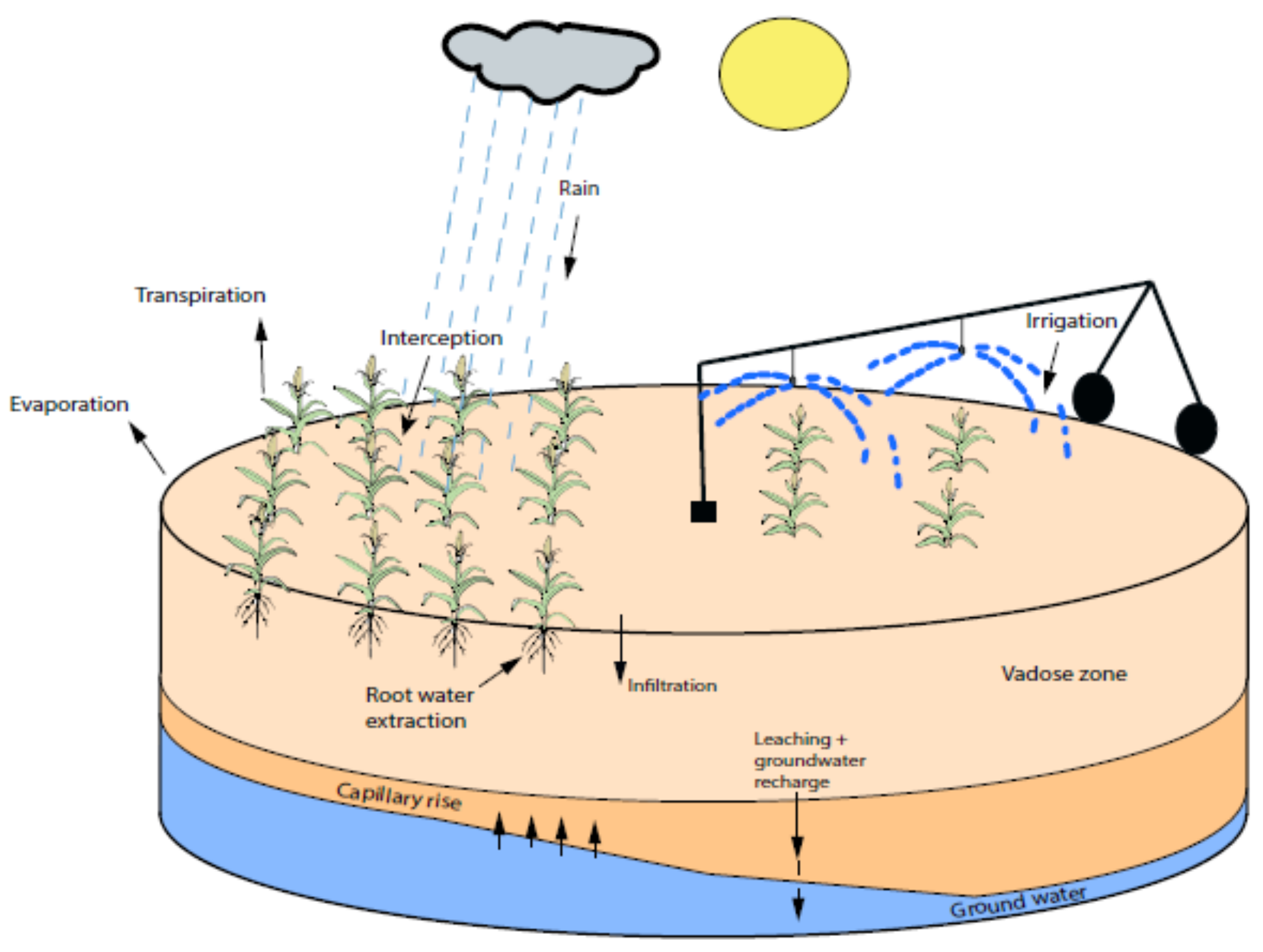
We considered an agro-hydrological system that characterizes the interaction between the soil, the water, the atmosphere, and the crop. The schematic of the considered agro-hydrological system is shown in Figure 1. The dynamics of the water flow in the agro-hydrological system can be represented by the Richards equation [23] as follows:
where h (m) is the field water pressure head; (mm) is the field water soil moisture content; (m) is the soil water capacity; (ms) is the hydraulic conductivity; z (m) is the vertical coordinate; (mms) is the source; and the sink term consists of plant-root water extraction.

Figure 1.
Schematic of an agro-hydrological system [24].
The details of the nonlinear relationship between hydraulic conductivity , capillary capacity , and soil moisture content () with pressure (h) can be found in [21,25,26]. The sink term in (1) characterizes the root-water extraction rate. The total root-water uptake depends upon the transpiration rate, the soil pressure head, and the root depth. The mathematical formulation of root-water uptake based on the Feddes model is expressed as follows [27]:
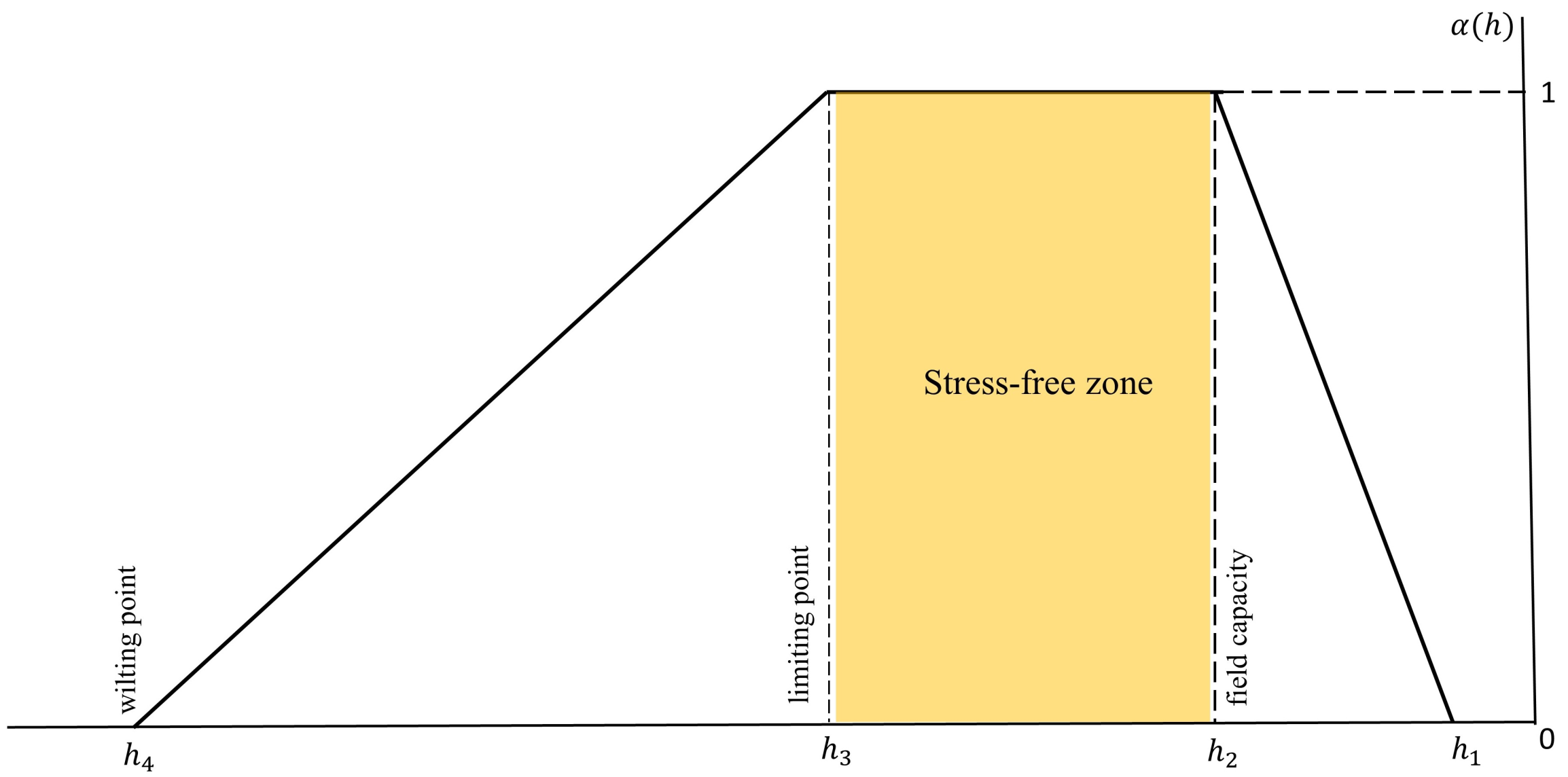
where [mms] is the maximum possible water-extraction rate under optimal conditions. [-] is the dimensionless water-stress factor. The water-stress factor depends upon the pressure head values and can be expressed as follows:
where is the pressure head value above which the root does not extract any water; and are the upper and lower threshold values, respectively, between which the root water extraction is maximum. is the permanent wilting point, below which the root water extraction is zero. The water-stress factor graph is shown in Figure 2. The stress-free zone is in between (field capacity) and (limiting point).
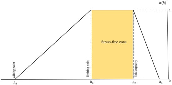
Figure 2.
Water stress factor graph.
The maximum possible water-extraction rate can be calculated using the Feddes model [27]:
where [ms] is the potential transpiration rate, and L [m] is the rooting depth. The potential transpiration rate is computed by:
where [ms] is the potential evapotranspiration rate, and [ms] is the potential evaporation rate. The can be expressed as follows:
where is the leaf area index. The potential evapotranspiration is computed as follows:
where [ms is the reference evaporation rate, which can be calculated based on the Penmon–Moneith equation [28], and [-] is the crop coefficient.
The crop-yield model is also important along with the Richards equation. The crop-yield model is modeled as a function of actual and potential evaporation and as follows:
where is the actual yield, and is the potential yield. is the crop-sensitivity factor at time k. T is the total time for growing seasons. is the actual evapotranspiration. can be represented as:
where is calculated from Equation (3), and is calculated from Equation (7).
In Equation (8), represents the yield deficiency, and represents the deficiency. By combining the Equations (8) and (9), the relationship between the crop yield and the soil pressure head is expressed as follows:
In this work, we considered that the agricultural field is equipped with a center-pivot irrigation system. A center-pivot irrigation system rotates across the field around a fixed pivot at the center of the field and irrigates in a circular manner. In order to account for the circular movement of the center-pivot irrigation system, the Richards equation in (1) is expressed in the cylindrical coordinates as follows [24]:
The three-dimensional agro-hydrological model in (11) is a nonlinear partial differential equation, which renders the problem difficult to solve analytically. In this work, we applied the explicit finite difference method to discretize the Richards equation in (11). Note that spatial discretization of the model was performed, such that a continuous-time state-space model was established as in the following form:
where denotes the states vector representing the pressure head value at each discretized node of total size , and represents the input vector containing irrigation values applied at each surface discretized node. As the input (irrigation amount) is applied to each surface node, it is incorporated in the system surface boundary condition. The surface boundary condition is characterized by the Neumann boundary condition as follows:
where h is the pressure head; is the input to the system; is the hydraulic conductivity; and is the height of the soil column. The bottom boundary condition is specified as free drainage.
2.2. Problem Formulation
As described in the previous section, the input u is only present at the top surface nodes. We also discussed that we considered a real agricultural farm that is facilitated with the central-pivot irrigation system. The circular motion of the central pivot allows to cover the entire farm area in a specified time i.e, the central pivot is not able to provide water to every plant at the same time. There is a rotational time gap for plants in receiving water. Therefore, we can say that that, at any instance, aligned to the central pivot where it irrigates, the current receiving region has some inputs u. As the whole region is discretized into a set of nodes, the current receiving region has nonzero nodes. Otherwise, the rest of the surface nodes are zero, which do not have any input. At each time, only some nodes have inputs, and it is changing over the rotation of the central pivot. Thus, this imposes a time-varying constraint on u as follows:
A continuous time state-space model with measurements and disturbances is considered as follows:
where denotes the soil pressure head measurements; is the weather disturbances.
The final objective was to calculate the optimum time and irrigation amount for maximum crop yield and water conservation for a three-dimensional field model with a central-pivot irrigation system.
3. Proposed Model Reduction
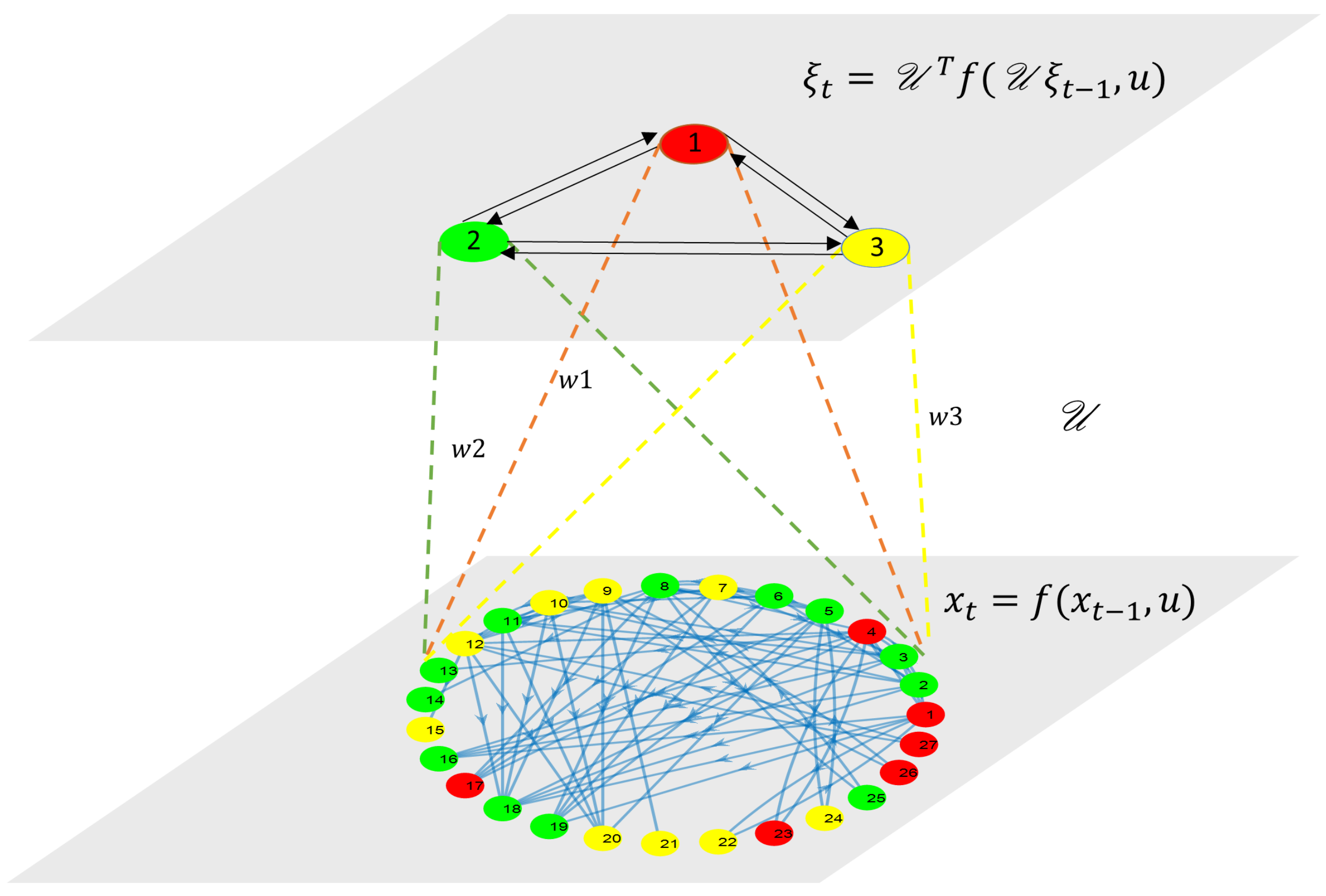
As discussed in the introduction, the finer discretization results in a large number of states for a large system. Thus, the use of the state-space model (12) is computationally expensive for the optimization step in the scheduler design where states are the decision variables in multiple-shooting- and collocation-based methods. Further, the optimization cost increases if the necessary and important state constraints are added for the system. The model reduction can deal with these issues. In classical model-reduction techniques, the states do not preserve the structure, so applying state constraints in a reduced model is difficult. Hence, we proposed a structure-preserving model-reduction technique. The calculation of a linear model in a large-scale system is also computationally expensive. So, in this work, we proposed the trajectory-based model-reduction techniques. The first step is to obtain the system trajectories. The second step includes the cluster calculations based on similarity among the trajectories. The third step calculates the projection matrix and constructs the reduced-order model using the Petrov–Galerkin projection. The illustration of the proposed model reduction is shown in Figure 3. The details of each step in the proposed algorithm are described as follows.
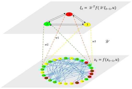
Figure 3.
Illustration of structure-preserving model reduction.
3.1. Step 1: Snapshot Matrix Generation
The first step is to generate the state trajectories. Based on the historical input from the scheduler or past year’s irrigation prescription, simulate the nonlinear system (12) and generate the state trajectories from the initial time to the final time as follows:
where is the snapshot matrix of the actual system; n is the number of states; and N is the total number of the sampling intervals.
3.2. Step 2: Calculation of Cluster Sets
In this step, the cluster matrix sets were generated. The main idea is to create clusters of states having similar dynamics based on the system trajectories. Then, the projection matrix is generated using the clustering information, and, using the projection matrix, the system is projected from a higher-dimensional system to a lower-dimensional reduced system. In this work, agglomerative hierarchical clustering [29] was used. We used the Euclidean distance between trajectories as the distance measure for states. The main reason to choose agglomerative hierarchical clustering is because of the capability to define the distance threshold between the clusters instead of predefining the number of cluster sets. The distance threshold is a tuning parameter for the accuracy of the reduced model. There are three commonly used linkage methods present in agglomerative hierarchical clustering (e.g., single, average, and complete linkage). In this work, we used the average linkage, and it considers the average distance between each point in one cluster to every point in other clusters.
where p and q are two clusters; i and j are data points within the clusters; d is the Euclidean distance between i and j; and are the size of the clusters of p and q, respectively.
Let us consider to be the collection of clusters after the hierarchical clustering, and r is the order of the resulted reduced model. The resulted clusters have the following properties: (i) and (ii) , where is the total number of states.
3.3. Step 3: Reduced-Model Construction
In this step, the reduced-order system is constructed based on the Petrov–Galerkin projection framework [17]. For the Petrov–Galerkin projection method, the projection matrix is required. After the construction of state clusters, the projection matrix is generated. The projection matrix is defined as , whose elements are expressed as follows:
and is determined as follows:
where ; is the norm of ; ; is the column of the identity matrix of size ; and m is the cardinality of set.
The adaptive reduced model of (12) is expressed as:
where and . Note that the actual state can be approximated based on mapping . The discrete model of (15) is expressed as follows:
The proposed reduced-order model can be used in different applications. The main advantages of using the reduced-order system are as follows:
- Proposed method preserves the connection structure among subsystems, while the general model techniques (POD, auto-encoder) do not preserve the structure.
- Due to preservation of structure, the proposed model reduction can be used in the distributed state estimation, distributed controller design, and sensor placement.
- The actual state constraints can be used for the reduced model using the projection matrix.
- The proposed model-reduction technique decreases the number of variables for a large-scale system, which makes the optimization problem tractable.
- Zone MPC—a reduction in the number of slack variables and constraints.
- Collocation-based method or multiple-shooting methods—a reduction in the number of state variables.
- The calculation of the jacobian matrix (which is useful for optimization and linearization) for the system is reduced to a very great extent.
4. Proposed Closed-Loop Scheduling
This section proposes closed-loop scheduling to calculate the time intervals between irrigation events and the water amount for each event. The primary objective is to maximize the crop yield while reducing the total water use and the equipment operating cost. The scheduler considers historical weather and the weekly weather forecast and the soil moisture measurements. The main idea is to irrigate the field and calculate the time required to reach the lower stress-free zone.
In this work, the iterative finite horizon optimization was considered like the classical MPC. However, the length of the horizon is not fixed because the time is also a decision variable in the optimization problem. The maximum time can be added in the constraint as a higher bound. The optimizer can make a prediction until the higher bound of time period and decide what is the optimum time within that limit. However, the weather forecast until the higher bound of time may not be accurate enough. So, the receding-horizon strategy was implemented to handle the uncertainty in the weather forecast. The optimization problem was resolved after an interval of a few days with a more-accurate weather forecast and recent measurements.
Each horizon consists of three separate segments. In the first segment, we irrigated the field, and the amount of water to be irrigated was the primary decision variable. In the second segment, the time was a decision variable that calculates the time for the next irrigation event. The time was calculated such that the plants will not experience stress, and the yield will be maximized. The third segment calculates the irrigation amount for the next horizon. The third segment is added to the optimization problem to give the optimizer some flexibility to see a few more days of future forecasts and make the irrigation time and amount more robust. In all three segments, the yield and the constraints were considered to keep the pressure head within a stress-free zone. The slack variables were introduced to relax the target zone. Note that the above three-segment design is inspired by the common practice used by farmers. This design can significantly reduce the computational complexity of the scheduler and lead to near-optimal solutions.
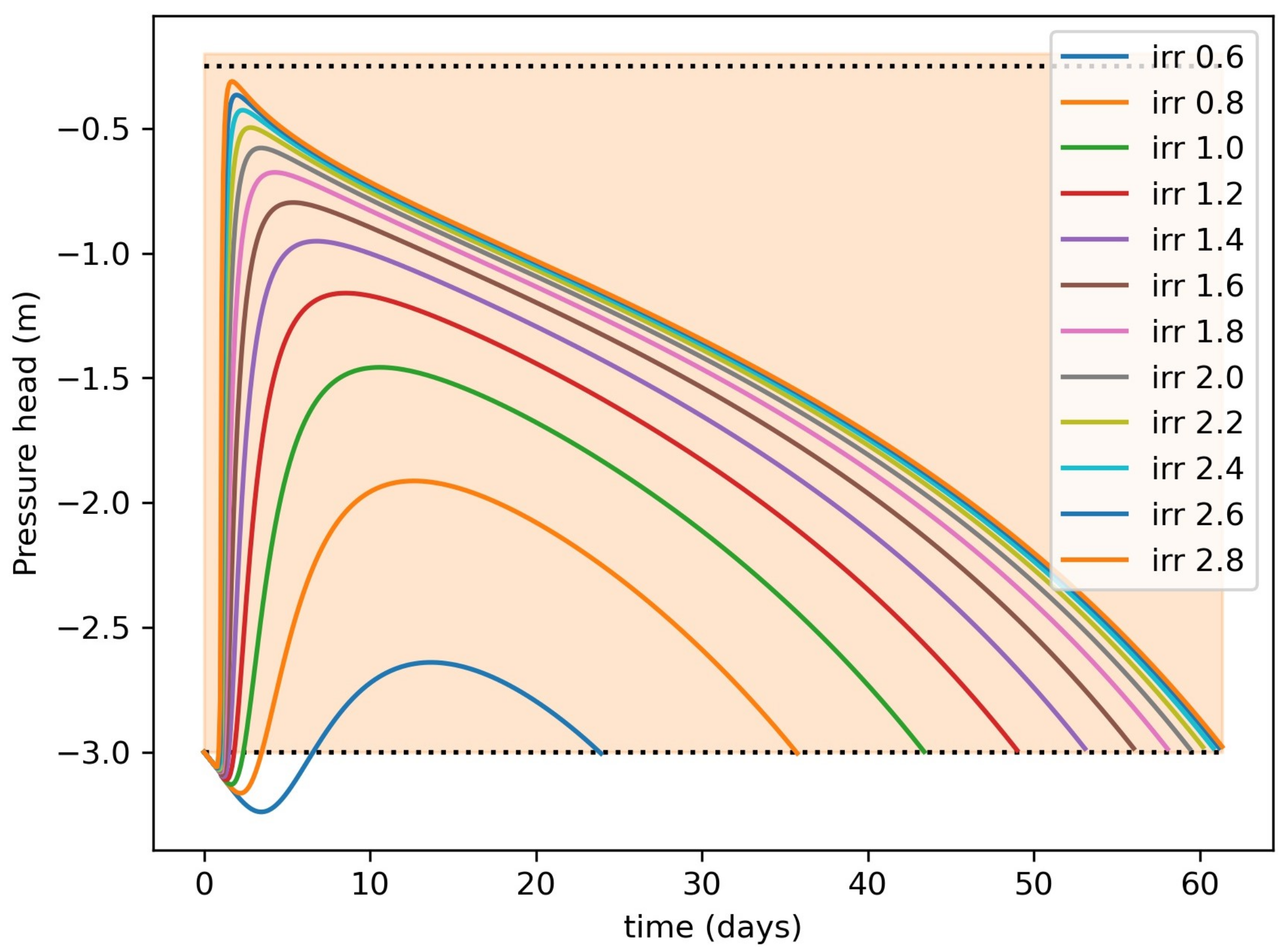
All three segments are optimized simultaneously. The reason to optimize everything together is that the amount of irrigation in the first and third segments will affect the total time in the second segment. The scenario may arise where we irrigate enough, but the total time for the next irrigation does not change much. This can be illustrated using a simple example. Let us consider the central-pivot irrigation system. The irrigation amount is changed gradually from m/s to m/s as shown in Figure 4. First, we irrigate the system and calculate the time when it reaches the lower zone. From Figure 4, we can observe that with the irrigation amount m/s, the number of days it reaches the lower zone in 23 days, and with the irrigation amount m/s, it takes around 61 days. It can also be observed that after a m/s irrigation amount, the number of days to reach the lower zone does not change much. Even if putting double the amount of water, the next irrigation days do not change significantly. So, if we optimize both the irrigation amount and the time together, we can save water and optimize the equipment functioning cost.
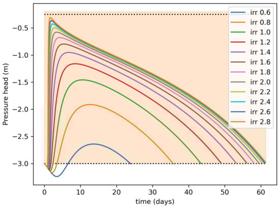
Figure 4.
Motivation of optimizing both input and time together. (irr represents the irrigation amount, and the units are in m/s).
For each horizon, the optimization problem is formulated as follows:
where Equation (17) defines the cost function to be minimized, and the input (u), time (T), and slack variables () are the decision variables. In Equation (17), the first term is the crop-yield deficiency cost; the second term considers the irrigation water cost; and the third term denotes the normalized time cost, which is active only in the second segment. The last term in Equation (17) is the cost term of non-negative slack variables (), which was introduced to relax the bounds of target zones in Equation (24). are the positive weighting factors. Equation (18) is the model used to evaluate the yield deficiency. Equations (19) and (20) represent the discrete time-reduced-order model and the output function. denotes current state estimates at time k. In this work, we assumed all the states can be estimated. is the number of the sampling time for first segment, and is the sampling time for the second segment (). Things to note include that in segment 2, the time was unknown, so the number of sampling points () is fixed and was chosen based on the upper bound of such that the model does not experience numerical issues. is the number of the sampling time for third segment. Equation (27) shows that the total sampling time is N. Equation (21) provides the bounds of input for the first segment and the third segment. Equation (22) defines the input amount as zero for the second segment. Equation (24) imposes the zone constraints with the slack variables and Equation (25) implies the slack variables are non-negative. Equation (26) defines the constraints for the lower and upper bounds of time.
As discussed before, the receding-horizon strategy was implemented to handle the weather uncertainty and use the scheduler as a closed-loop system. The day () until which we can forecast the accurate weather condition was selected. In general, we forecast the weather for seven days. So, if the scheduler predicted the next irrigation event to more than seven days, then we reevaluated the scheduler optimization after seven days again with the current field condition as the initial condition and the future seven days weather forecast. If the scheduler predicts the irrigation event less than seven days, then we solved the optimization problem for the next horizon using the recent day field condition as the initial condition. The algorithms for the receding horizon are as follows:
- At the current time (k) solve the optimization problem (4), with initial condition and obtain the optimum input (u) and time (T).
- If the optimum time (T) is greater than (), then resolve the optimization problem (4) with initial condition and obtain the optimum input and time.
- Else () solve the optimization problem (4) with initial condition and obtain the input and time.
5. Results
In this section, the proposed algorithms are applied to demonstrate the performance of reduced-order model and the scheduler under different scenarios. A field of radius 50 m and depth 30 cm was considered. The 30 cm depth was selected because, for the crops selected in this work, the maximum root-water extraction happens in between the depth of 30 cm. The field was equipped with a central-pivot irrigation system. The model of the farm was constructed using finite-difference discretization of the Richards equation. The entire system was discretized into 1920 nodes with 5 in radial, 64 in azimuthal, and 6 in axial directions. Each node corresponds to a state of the system. The central pivot takes around 8 h to irrigate the whole field. Different types of crops and soil types were considered in different scenarios.
5.1. Results: Model Reduction
In this subsection, the proposed model reduction discussed in Section 3 is applied to the system. First, the effect of the reduced-model order on the mean square error (MSE) of the reduced model is discussed. Then, the robustness of the reduced model is discussed.
In this simulation, we considered the real soil properties of the field located at Lethbridge, Canada. In summer 2019, we collected soil samples at 20 points in the field, and in the soil lab the soil types were estimated. We found three different soil types present in the field: loam, sandy clay loam, and clay loam. The hydraulic properties of the soil types are shown in Table 1 [30]. The kriging method was applied to get the soil properties of all other nodes of the field. Figure 5 shows one selected parameter () of the surface nodes. The other parameters also followed the same trend.

Table 1.
Soil properties of three different types of soil.
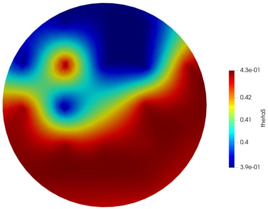
Figure 5.
Model parameter
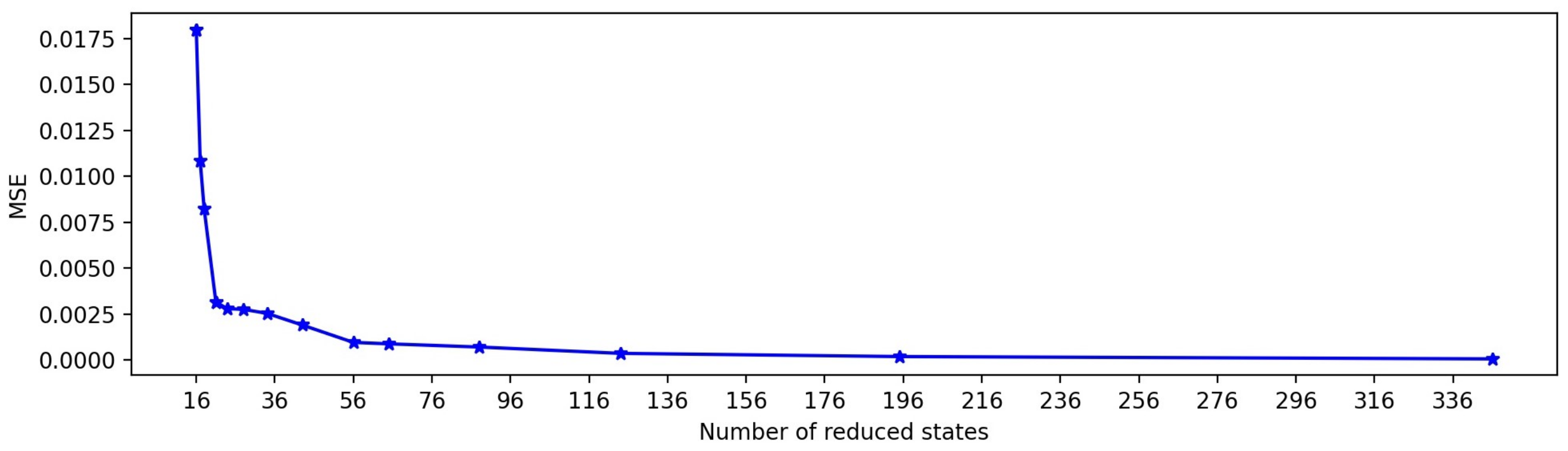
Figure 6 shows the MSE values of the reduced model with the number of reduced states. The number of reduced states was obtained by changing the threshold values of the agglomerative hierarchical clustering method starting from 0.3 to 3.5 by increasing 0.2. As discussed in Section 2, we can specify the threshold values in hierarchical clustering instead of the number of reduced models. The MSE values are calculated between the actual model and the reduced-order model. From Figure 6 it can be observed that after 56 reduced states, the error values are minimal. For this simulation, we consider 30 reduced states.
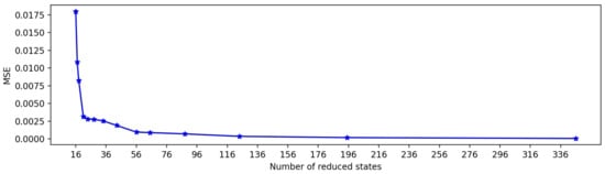
Figure 6.
Values of MSE with different reduced order.
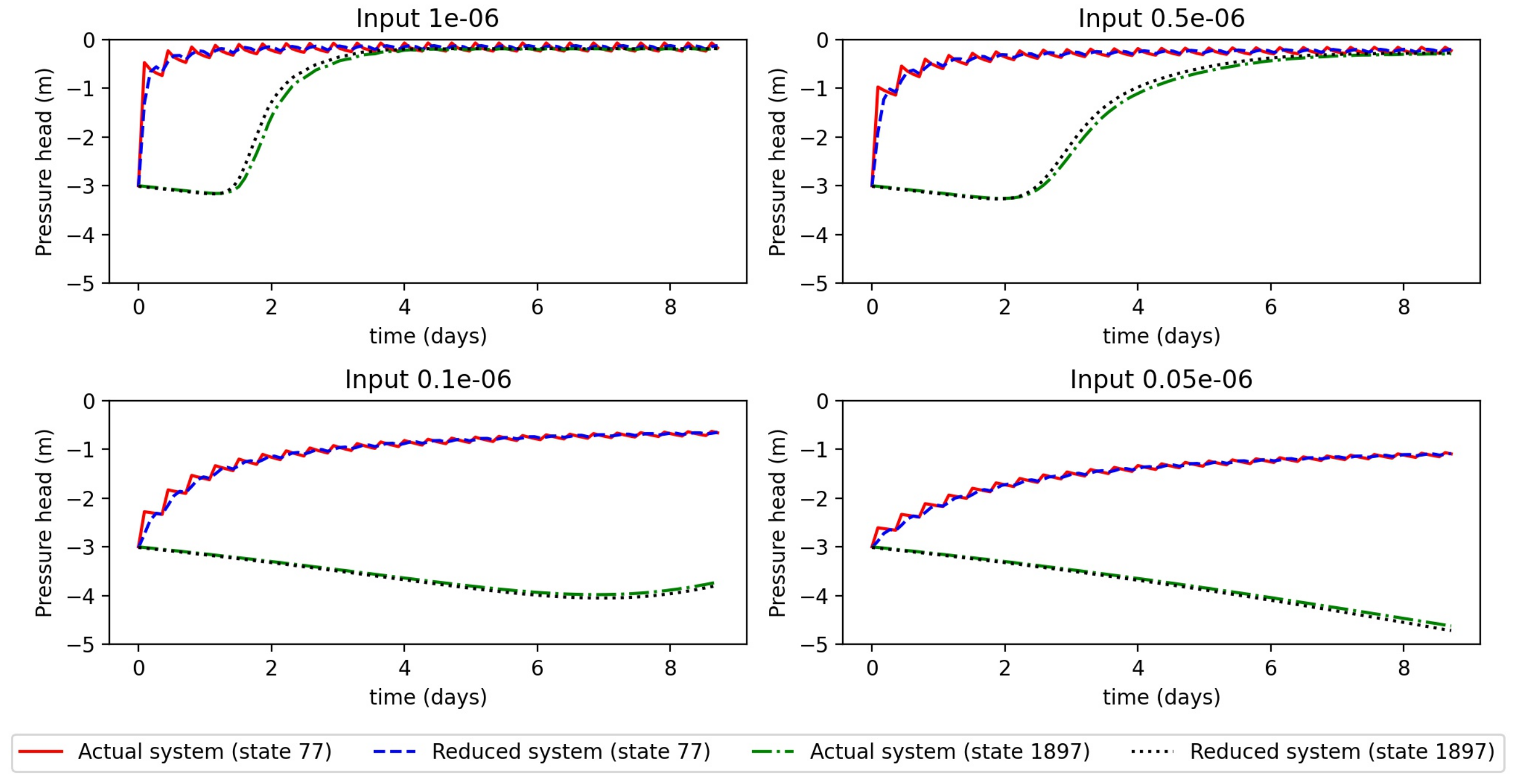
Next, we presented the robustness of the reduced model. In the optimization-based controller design, the input amount is one of the important decision variables. So, the reduced model should be robust enough to handle different input amounts. First, the projection matrix was calculated using the initial condition −4.0 m and input amount m/s. Then, using the same projection matrix, we simulated the reduced-order model starting from a different initial condition (−3.0 m) and different input amounts ( m/s, m/s, m/s, and m/s). Figure 7 shows the state trajectories of the actual system and the reduced-order system randomly chosen state 77 (surface) and 1897 (depth 25 cm) for different input amounts. It can be observed that reduced-order trajectories are very close to the actual order trajectories, which shows the robustness of the proposed model-reduction method.
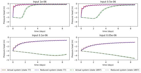
Figure 7.
Trajectories of some selected states of the actual system and reduced system for four different inputs.
5.2. Result: Scheduler
In this subsection, the performance of the proposed scheduler design is demonstrated under the following three scenarios: (1) Scenario 1: uniform soil types, no rain, constant ET and grass; (2) Scenario 2: non-uniform soil types, no rain, constant ET and grass; (3) Scenario 3: uniform soil, dry bean crop type, variable ET and rain.
5.2.1. Scenario 1
In this subsection, we consider a simple scenario of a uniform soil type of loam. We further assumed that there are no disturbances present like rain and variable ET. We considered the crop as grass. The simple scenario was considered to show how the proposed scheduler algorithm works.
We considered the 2nd layer from the top as the root zone of the grass, which is the output to the optimization problem (Equation (20)). The values of the tuning parameters , , , , and were 1, 1, 1, 100, and 1, respectively. In this scenario, we put more weight on to make the system not violate the lower bound, which is more crucial for the zone control. As described in the previous sections, it is difficult to get back to normal again if the plant gets stressed once. The actual upper and lower bounds of the system for the maximum yield and stress-free zone were −0.25 m and −3.1 m [31], respectively. Points to note include that the stress-free zone depends upon different types of crop and ET values. To ensure the system does not experience the actual stress, a more-conservative zone was considered with lower and upper zones −2.8 m and −1.0 m, respectively. So, even if the system violates the more-conservative zone, it does not experience the actual stress. The lower bound and the upper bound of input were considered as 0 m/s and m/s, respectively. The lower bound of time was considered 30 min, while the upper bound was kept as 16 days.
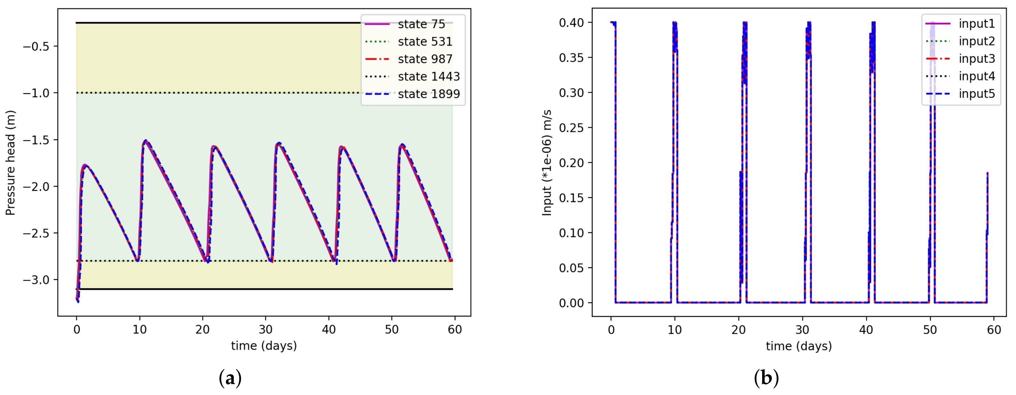
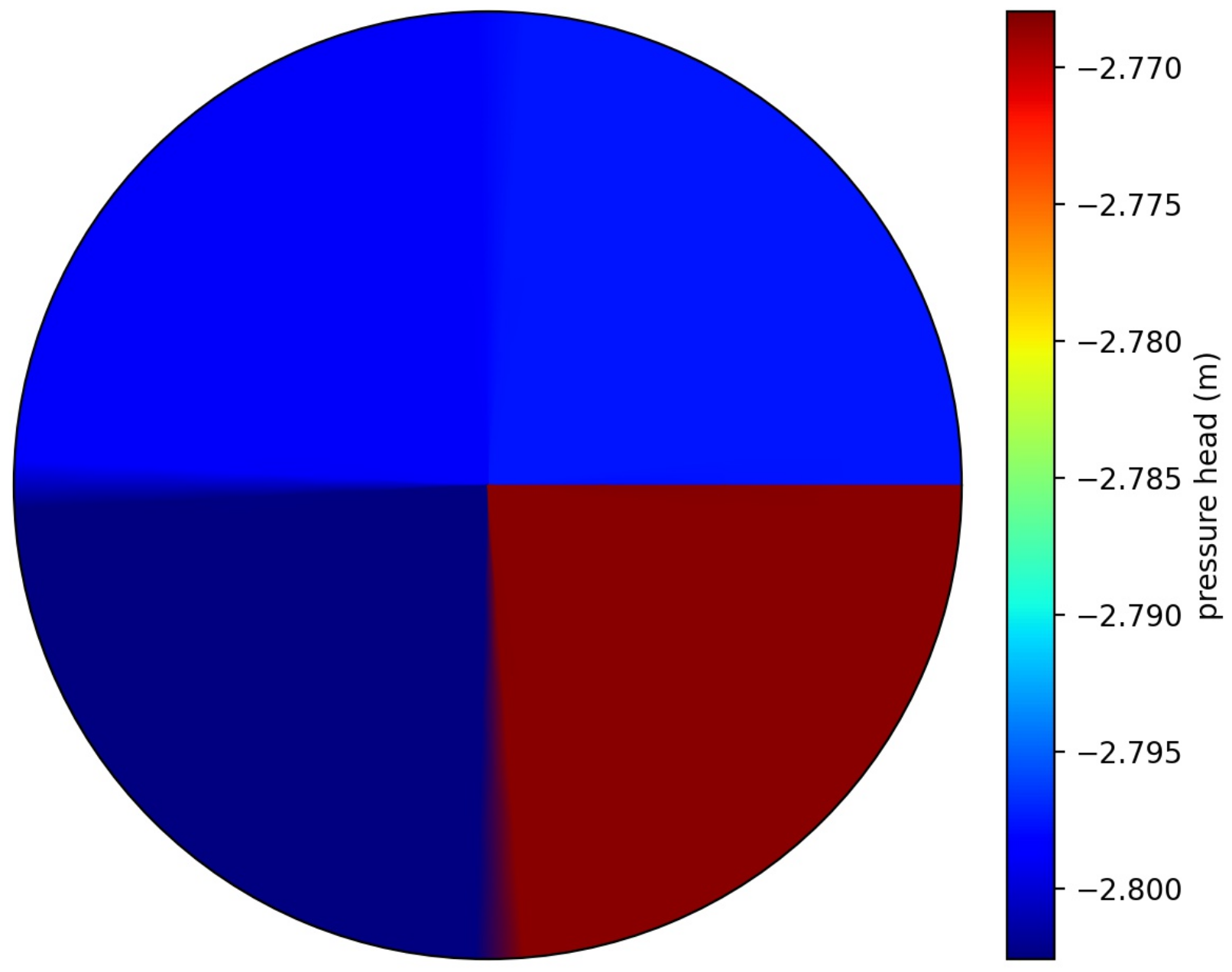
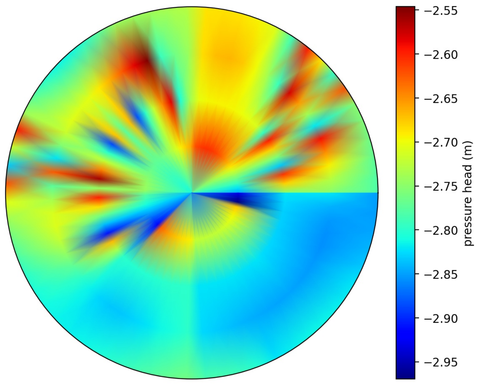
Figure 8a shows the states trajectories of five randomly selected states on the 2nd layer, and Figure 8b shows the input amount. From Figure 8a, we can observe that after it reaches the conservative lower zone, the system irrigates again. The root zone remains within the zone all the time so that the plants never get stressed. Figure 8b shows the input amount for all the five sprinklers. As the farm has a uniform soil type, all the sprinklers give nearly the same value. We can also observe that the irrigation event can be planned after nearly a ten-day interval. Figure 9 shows the 2nd-layer pressure head values. We can observe that all the nodes were around −2.8 m, which is the conservative lower zone value. In all the quadrants, we observed slightly different pressure head values because of the central pivot rotation.
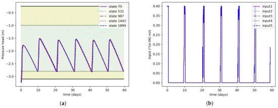
Figure 8.
(a) Selected state trajectories under the proposed zone scheduler design for scenario 1; (b) irrigation amount for 5 different sprinklers obtained from proposed zone scheduler.

Figure 9.
Pressure head values for root-zone layer.
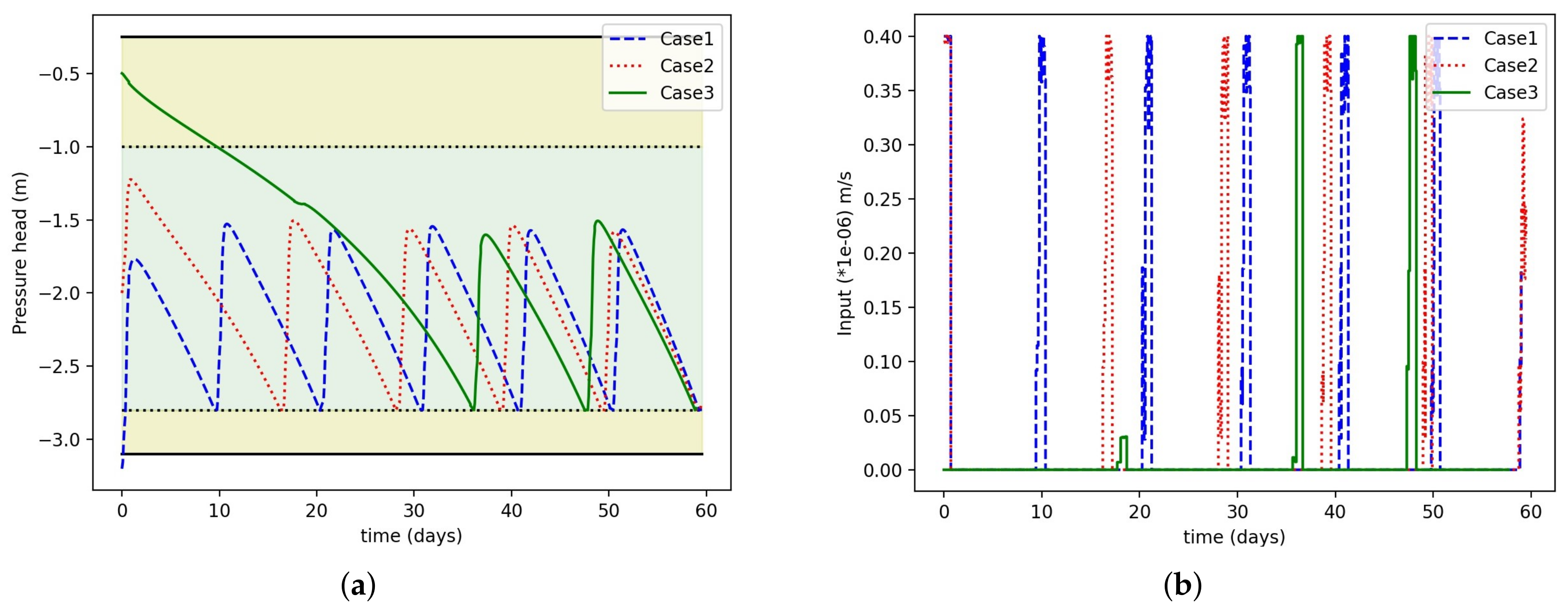
Further, the robustness of the proposed scheduler was analyzed. We considered three different cases based on initial conditions (−0.5 m, −3.2 m, and −2.0 m). The initial conditions were chosen such that two initial conditions are outside of the zone and one is already inside the zone. Figure 10a presents the state trajectory of one randomly selected state 75 on the 2nd layer. It can be observed that in all three cases, the scheduler worked fine. Figure 10a shows the input profile for sprinkler 1 for all the three cases. We can see that in case 1 the irrigation amount was higher than the other two cases. This is because the initial condition is outside the lower zone and requires more and frequent irrigation to keep within the zone. In case 3, as the initial condition was already very wet, the scheduler prescribed very little water until it reached the lower zone.
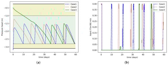
Figure 10.
(a) Selected state trajectories for three cases (different initial conditions); (b) input trajectories for three cases.
5.2.2. Scenario 2
In this scenario, we considered the non-uniform soil types, no rain, and constant ET. The motive was to show the efficiency of the scheduler in the presence of different soil types. The soil arrangement discussed in Section 5.1 was considered in this scenario (Figure 5). We considered the 3rd layer from the top (10 cm depth) as the root zone of the crop-type grass. The scheduler tried to keep only the 3rd layer inside the zone. The values of the upper and lower bounds of the actual and conservative zones were the same as in scenario 1. The lower and upper bounds of inputs were 0 m/s and m/s, respectively. The lower and upper bounds of the time were 30 min and 12 days, respectively.
Figure 11a shows state trajectories of some selected states from the 3rd layer. It shows that the states stay within the zone, and some of the states were slightly outside of the conservative zone. It may be caused because of the reduced-model error and different soil types. All the states’ values for the 3rd layer at the end time are shown in Figure 12. We can observe that the all the pressure head values were above the lower zone value of −3.1 m. Figure 11b shows the input trajectories of five different sprinklers obtained form the scheduler. As observed from the figure, the input amounts were not same for all the sprinklers. This shows that for different soil types, the sprinklers may put different amounts of water.
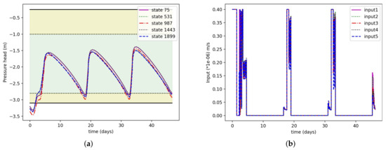
Figure 11.
(a) Selected state trajectories at 3rd layer under the proposed zone-scheduler design for scenario 2; (b) irrigation amount for 5 different sprinklers obtained from the proposed zone scheduler.

Figure 12.
Pressure head values of a depth of 10 cm.
5.2.3. Scenario 3
In this scenario, the variable ET and rain uncertainties are considered. The uniform soil type of loam and the crop type of lettuce were chosen for the simulation. This scenario was shown to check the efficacy of the scheduler in the presence of weather disturbances and crop-growth stages. As discussed in the crop modeling, 85% root water was extracted from the top 30 cm of soil. For the high yield and the crop not to experience any stress, keeping the top 30 cm in the stress-free zone is required. In this scenario, the objective of the scheduler was to keep all the layers in the zone. The values of the upper and lower bounds for the actual zone were −0.25 m and −3.1 m, respectively. The upper and lower bounds for the conservative zone were considered as −0.5 m and −2.3 m, respectively. The values of the tuning parameters , and were 1, 100, 1, 100, 0.01, and 1, respectively. Points to note include that the tuning-parameter values can be adjusted depending on the root growth with time. The lower and upper bounds of the time were 30 min and 12 days, respectively. The upper and lower bounds of the input were 0 m/s and m/s, respectively. In general, a seven-day rain forecast can be 80% accurate. So, for one horizon in the scheduler, the accurate weather forecast of 7 days was used, and for the rest of the days, the long-term forecast value was used. The values of the accurate weather forecast and the long-term weather forecast considered for this simulation are shown in Figure 13a. Similarly, the reference ET value for the accurate and the long-term weather forecast is shown in Figure 13b. The crop coefficient () for the lettuce crop type for all the growing season is shown in Figure 13c. All growing seasons consisted of the initial, crop-development, mid-season, and late seasons.
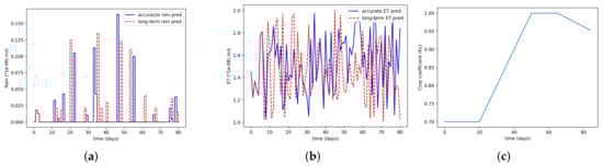
Figure 13.
(a) Accurate rain forecast and long-term rain forecast; (b) accurate ET forecast and long-term ET forecast, (c) crop coefficient for total growing season for lettuce.
Figure 14a shows some selected state trajectories at different depths. We can observe that for all the depths, the states were in the stress-free zone. We can also see that around 50 days, state 60 (bottom node) goes outside of the conservative zone. This happens because around day 50, the crop is at the mature stage, and the ET values are high Figure 13c, and there is some delay between the water to reach the bottom node. That is why we choose a conservative zone of −2.3 m. So, even if the bottom nodes go outside of the conservative zone, it may have less chance to go outside of the actual stress zone. Figure 14b shows the input amount for all five sprinklers. We can observe that there is frequent irrigation at the beginning because the states are outside of the zone. Moreover, around days 45–50, there was frequent irrigation because of high ET values, and the crop needed more water at that stage. For other days, because of rain and low ET values, the scheduler prescribed less frequent irrigation.
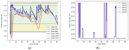
Figure 14.
(a) Selected state trajectories for all layers under the proposed zone-scheduler design for scenario 3; (b) irrigation amount for 5 different sprinklers obtained from proposed scheduler for scenario 3.
6. Conclusions
In this article, the closed-loop scheduler for a large agro-hydrological system was proposed. The cylindrical version of the finite-difference model was explicitly constructed for an agricultural field equipped with a central pivot. The algorithm for the proposed structure-preserving model reduction was discussed. The motivation and the algorithm of the proposed scheduler were presented. The scheduler optimized the irrigation amount and time of the following irrigation event to assure maximum yield, water preservation, and electricity usage. The proposed approach was applied to three different cases. In all the cases, the proposed scheduler showed a satisfactory result.
Author Contributions
Conceptualization, S.R.S. and J.L.; methodology, S.R.S., B.T.A., S.D. and J.L.; software, S.R.S.; validation, S.R.S.; investigation, S.R.S.; data curation, S.R.S.; writing—original draft preparation, S.R.S. and S.D.; writing—review and editing, J.L.; supervision, J.L.; All authors have read and agreed to the published version of the manuscript.
Funding
Financial support from the National Sciences and Engineering Research Council of Canada (NSERC) and Alberta Innovates is greatly acknowledged.
Institutional Review Board Statement
Not applicable.
Informed Consent Statement
Not applicable.
Data Availability Statement
The data presented in this study are available on request from the corresponding author.
Conflicts of Interest
The authors declare no conflict of interest.
References
- World Economic Forum. The Global Risks Report, 10th ed.; Technical Report; World Economic Forum: Geneva, Switzerland, 2015. [Google Scholar]
- United Nations World Water Assessment Programme. Waste Water the Untapped Resource; Technical report; United Nations: New York, NJ, USA, 2017. [Google Scholar]
- Lozoya, C.; Mendoza, C.; Mejía, L.; Quintana, J.; Mendoza, G.; Bustillos, M.; Arras, O.; Solís, L. Model predictive control for closed-loop irrigation. IFAC Proc. Vol. 2014, 47, 4429–4434. [Google Scholar] [CrossRef] [Green Version]
- Goodchild, M.; Kühn, K.; Jenkins, M.; Burek, K.; Button, A. A method for precision closed-loop irrigation using a modified PID control algorithm. Sens.Transducers 2015, 188, 61. [Google Scholar]
- McCarthy, A.C.; Hancock, N.H.; Raine, S.R. Simulation of irrigation control strategies for cotton using Model Predictive Control within the VARIwise simulation framework. Comput. Electron. Agric. 2014, 101, 135–147. [Google Scholar] [CrossRef] [Green Version]
- Delgoda, D.; Malano, H.; Saleem, S.K.; Halgamuge, M.N. Irrigation control based on model predictive control (MPC): Formulation of theory and validation using weather forecast data and AQUACROP model. Environ. Model. Softw. 2016, 78, 40–53. [Google Scholar] [CrossRef]
- Thorp, K.R.; Hunsaker, D.J.; Bronson, K.F.; Andrade-Sanchez, P.; Barnes, E.M. Cotton Irrigation Scheduling Using a Crop Growth Model and FAO-56 Methods: Field and Simulation Studies. Trans. ASABE 2017, 60, 2023–2039. [Google Scholar] [CrossRef] [Green Version]
- Cahoon, J.; Ferguson, J.; Edwards, D.; Tacker, P. A Microcomputer-Based Irrigation Scheduler for the Humid Mid-South Region. Appl. Eng. Agric. 1990, 6, 289–295. [Google Scholar] [CrossRef]
- Jensen, M.E.; Robb, D.C.; Franzoy, C.E. Scheduling Irrigations Using Climate-Crop-Soil Data. J. Irrig. Drain. Div. 1970, 96, 25–38. [Google Scholar] [CrossRef]
- Bras, R.L.; Cordova, J.R. Intraseasonal water allocation in deficit irrigation. Water Resour. Res. 1981, 17, 866–874. [Google Scholar] [CrossRef]
- Wardlaw, R.; Barnes, J. Optimal Allocation of Irrigation Water Supplies in Real Time. J. Irrig. Drain. Eng. 1999, 125, 345–354. [Google Scholar] [CrossRef]
- Hassan-Esfahani, L.; Torres-Rua, A.; McKee, M. Assessment of optimal irrigation water allocation for pressurized irrigation system using water balance approach, learning machines, and remotely sensed data. Agric. Water Manag. 2015, 153, 42–50. [Google Scholar] [CrossRef]
- Nahar, J.; Liu, S.; Mao, Y.; Liu, J.; Shah, S.L. Closed-Loop Scheduling and Control for Precision Irrigation. Ind. Eng. Chem. Res. 2019, 58, 11485–11497. [Google Scholar] [CrossRef]
- Kassing, R.; De Schutter, B.; Abraham, E. Optimal Control for Precision Irrigation of a Large-Scale Plantation. Water Resour. Res. 2020, 56, e2019WR026989. [Google Scholar] [CrossRef]
- Agyeman, B.T.; Sahoo, S.R.; Liu, J.; Shah, S.L. LSTM-based model predictive control with discrete actuators for irrigation scheduling. In Proceedings of the 13th Symposium on Dynamics and Control of Process Systems (DYCOPS), Busan, Korea, 14–17 June 2022. submitted. [Google Scholar]
- Babaeian, E.; Sadeghi, M.; Jones, S.B.; Montzka, C.; Vereecken, H.; Tuller, M. Ground, proximal, and satellite remote sensing of soil moisture. Rev. Geophys. 2019, 57, 530–616. [Google Scholar] [CrossRef] [Green Version]
- Antoulas, A. Approximation of Large-Scale Dynamical Systems; Society for Industrial and Applied Mathematics: Philadelphia, PA, USA, 2005. [Google Scholar]
- Ishizaki, T.; Kashima, K.; Imura, J.; Aihara, K. Model reduction and clusterization of large-scale bidirectional networks. IEEE Trans. Autom. Control 2014, 59, 48–63. [Google Scholar] [CrossRef]
- Cheng, X.; Kawano, Y.; Scherpen, J.M.A. Graph structure-preserving model reduction of linear network systems. In Proceedings of the 2016 European Control Conference (ECC), Aalborg, Denmark, 29 June–1 July 2016; pp. 1970–1975. [Google Scholar]
- Cheng, X.; Scherpen, J.M.A. Gramian-based model reduction of directed networks. arXiv 2019, arXiv:1901.01285. [Google Scholar]
- Sahoo, S.R.; Yin, X.; Liu, J. Optimal sensor placement for agro-hydrological systems. AIChE J. 2019, 65, e16795. [Google Scholar] [CrossRef]
- Sahoo, S.R.; Agyeman, B.T.; Debnath, S.; Liu, J. Knowledge-based optimal irrigation scheduling of three-dimensional agro-hydrological systems. In Proceedings of the 13th Symposium on Dynamics and Control of Process Systems (DYCOPS), Busan, Korea, 14–17 June 2022. submitted. [Google Scholar]
- Richards, L.A. Capillary conduction of liquids through porous mediums. Physics 1931, 1, 318–333. [Google Scholar] [CrossRef]
- Agyeman, B.T.; Bo, S.; Sahoo, S.R.; Yin, X.; Liu, J.; Shah, S.L. Soil moisture map construction using microwave remote sensors and sequential data assimilation. J. Hydrol. 2021, 598, 126425. [Google Scholar] [CrossRef]
- Mualem, Y. A new model for predicting the hydraulic conductivity of unsaturated porous media. Water Resour. Res. 1976, 12, 513–522. [Google Scholar] [CrossRef] [Green Version]
- van Genuchten, M.T. A Closed-form Equation for Predicting the Hydraulic Conductivity of Unsaturated Soils1. Soil Sci. Soc. Am. J. 1980, 44, 892. [Google Scholar] [CrossRef] [Green Version]
- Feddes, R.A. Simulation of Field Water Use and Crop Yield; Pudoc: Wageningen, The Netherlands, 1982; pp. 194–209. [Google Scholar]
- Allen, R.G.; Pereira, L.S.; Raes, D.; Smith, M. Crop Evapotranspiration-Guidelines for Computing Crop Water Requirements-FAO Irrigation and Drainage Paper 56; FAO: Rome, Italy, 1998; Volume 300, p. D05109. [Google Scholar]
- Steinbach, M.; Karypis, G.; Kumar, V. A comparison of document clustering techniques. In KDD Workshop on Text Mining; Department of Computer Science/Army HPC Research Center: Minneapolis, MN, USA, 2000. [Google Scholar]
- Carsel, R.F.; Parrish, R.S. Developing joint probability distributions of soil water retention characteristics. Water Resour. Res. 1988, 24, 755–769. [Google Scholar] [CrossRef] [Green Version]
- Feddes, R.; Raats, P. Parameterizing the soil—water—plant root system. Unsaturated-Zone Model. Progress Challenges Appl. 2004, 6, 95–141. [Google Scholar]


Publisher’s Note: MDPI stays neutral with regard to jurisdictional claims in published maps and institutional affiliations. |
© 2022 by the authors. Licensee MDPI, Basel, Switzerland. This article is an open access article distributed under the terms and conditions of the Creative Commons Attribution (CC BY) license (https://creativecommons.org/licenses/by/4.0/).