Environmental Externalities of Secondhand Markets—Based on a Dutch Auctioning Company

Abstract

Buying reused products rather than new ones could reduce the emissions of greenhouse gases (GHGs). There are many aspects that can influence whether used products actually cause emissions to increase or decrease. This paper assesses the effects of secondhand markets on GHG emissions by using data on twelve product categories from Troostwijk Auctions, which is a Dutch auctioning company. Data came from a carbon footprint database, survey data and many other sources. The net impact of secondhand trade is calculated by combining existing formulas in the literature and by performing regressions to estimate the values of unknown data. A methodology is proposed to find appropriate assumptions to handle uncertainty of carbon footprints. The main result is that the emission savings due to reuse of almost all products in the analysis are offset because many buyers purchase goods that they would not have bought new. Trade in the vehicles included in this study even adds emissions.

1. Introduction

A major challenge of this time is the combat against climate change and global warming, which is caused by an excessive presence of GHGs in the atmosphere [1]. Rising temperatures lead to threats not only to animal life, but also to plants and crops. Moreover, they will make the weather dangerously extreme. The most common greenhouse gas is carbon dioxide (CO₂). Other greenhouse gases include water vapor, methane, ozone, chlorofluorocarbons and nitrous oxide (N₂O), and although these may have a greater global warming potential (GWP) than CO₂, their concentrations in the atmosphere are far lower than that of CO₂.

To mitigate the process of climate change and global warming, emissions must decrease [1]. There are many ways to achieve a decrease in GHG emissions, including an increased usage of renewable energy sources and higher energy efficiency. Another way to reduce GHG emissions is through reuse and recycling strategies, which are also the focus of this paper.

This paper investigates the sustainability and externalities of reuse or, more specifically, the product life extension because of reuse. For example, online trade in used goods has been estimated to reduce emissions by around 650,000 tonnes of CO_2e in Germany in 2011 when compared to new purchases of those same goods [2]. At that time, total national GHG emissions were approximately 850 million tonnes. Online marketplaces are widely used. In the Netherlands, 32% of the population of over 12 years old bought a secondhand good online in 2019 [3]. The question that will be addressed in this paper, is:

What are the external effects of an online business-to-business marketplace due to GHG emissions?

After a literature review on existing literature in Section 2, the data and methodology are presented in Section 3. The Dutch auctioning company Troostwijk Auctions will serve as a case study. Data from Troostwijk Auctions are used. The company has data on a multitude of product categories, ranging from furniture to crop harvesters. Twelve product types are chosen that should give a diverse image of the GHG impact of this online platform. Calculations are performed by combining data from various sources on carbon footprints, product lifespans, efficiency changes, the reported residual lifetime of used goods, and the reported number of new items displaced by secondhand transactions. Uncertainty is handled with Monte Carlo simulation.

For each product type, the environmental externalities of the secondhand sale of an average lot will be assessed as precisely as possible. Note that a lot is any auctioned good. After, the results will be extrapolated to entire product types, and regressions will be run to perform this extrapolation in a satisfying way. The results are discussed in Section 4. As used goods only displace the production of 0.2–0.35 new goods, the resale of most product categories in this study has an ambiguous effect on GHG emissions, and the vehicle categories increase emissions. Section 5 discusses the research and concludes.

2. Literature Review

This paper contributes to the knowledge on the environmental externalities of secondhand platforms. Little has been written about secondhand markets for durable goods in general [4]. Research has more often aimed at the cases of, for example, clothing or books [4,5]. This research can be viewed as a consequential life cycle assessment (LCA) [6]. LCAs can help companies to optimize their environmental impact and can show where collaboration is needed [7]. Moreover, it can help policymakers make sustainable plans and rank the impact of changes so that policymakers know which plans should have the highest priority. Aiding companies, consumers and policymakers is becoming increasingly relevant, as people become increasingly worried about climate change [8]. Additionally, limited knowledge about environmental sustainability is one of the top barriers to sustainable practices for small and medium-sized companies, which form 90 percent of the world’s businesses [9].

Reuse and product life extension are intimately related, and there have been many studies on optimal lifespans of goods [10]. For example, Schaubroeck et al. [6] developed a framework for the decision on when to replace car and Bakker et al. [11] found that refrigerators and laptops should be used for 20 and 7 years instead of the observed 14 and 4 years, respectively.

There exists a study about the GHG emissions of the German version of eBay [2]. This research quantified eBay’s environmental impact by calculating the magnitude of a number of different variables for different product types. This is also the aim of the present paper. The paper on eBay concluded that reusing is better than new purchases, except for the case of powered products with a relatively large carbon footprint. However, not only is that paper a decade old, eBay is a very different platform than Troostwijk Auctions. Where eBay is aimed at consumers, Troostwijk Auctions is a business-to-business corporation, causing sold lots to more often be industrial. This means that products will almost never be sent by post, contrary to the case of eBay. Moreover, the research on eBay used data from ecoinvent, which is not freely accessible, and uncertainty was often not accounted for.

An example of a commercial rather than scientific paper about this topic is that concerning and commissioned by the Dutch website Marktplaats [12]. It concluded that reusing in the cases of four groups of products in its sample saved emissions. These groups were small electronics, furniture, clothing, and baby beds and transport. The research on Marktplaats does not explicitly state its method to deal with uncertainty ranges and uses ecoinvent, similar to the study on eBay. What is more, the calculations assume that used goods displace new goods one-to-one, which is an unrealistic assumption [5,10,13,14], and exclude transportation emissions and efficiency changes in the utilization phase.

The assumptions on the number of new goods displaced by used goods, the so-called displacement rate, has been subject to several studies. For example, Fortuna & Diyamandoglu [5] developed a framework to optimize the share of discarded goods that should be reused. In a research on the coss-price elasticities of new and used materials, Zink et al. [13] find that one-to-one displacement rarely occurs and that displacement is especially low when used materials are inferior to new ones. Thomas [14] shows that secondhand markets can even increase demand for new goods when used goods become scarce.

This research addresses a gap in the literature since there is still much to be written on secondhand markets, and there have been only few assessments of the environmental impact of online marketplaces. This paper makes a contribution to the existing research by developing a reproducible methodology and conducting a case study on a business-to-business marketplace, which has, to the authors’ best knowledge, not been carried out before.

In

Table 1. Some aspects influencing the environmental effects of secondhand trade are included in this study, others are excluded.

Aspect	Included?
Delayed or prevented manufacturing and end-of-lofe (EoL) emissions [5,10]; the EoL phase can also reduce emissions due to recycling [10].	Yes
Higher energy efficiency of newly manufactured goods [2,6,10,14]	Yes
Transportation emissions [2,5]	Yes
A displacement rate below 1, i.e., not all buyers of used goods would alternatively have purchased a new good [5,10,13,14].	Yes
Changing efficiency over a good’s lifetime [10,11,15]	No
Decreasing product lifespans [11]	No
Acceleration of consumption [2] because of the existance of a secondhand market [10] and less minimalist attitudes [4,14]	No
A rebound effect due to the monetary gains from secondhand trade [2,7,14]	No
Different recycling effectiveness internationally, formally or informally, when used goods are sold to other countries [16,17].	No
Used goods replacing even older goods [18]	No
Higher environmental impact of cheap new goods than of higher-quality new goods [2]	No
Used goods displacing goods of other types [13]	No

, the aspects relevant to the environmental impact of reselling a good are mentioned that are found in the literature. Some of those aspects will be included in the calculations, some of them will be left out. The decision not to include aspects in the calculations is usually made due to low data availability or ambiguity of the effect of the aspect. They should still not be forgotten when interpreting the results.

3. Materials and Methods

3.1. Unit of Measurement

Different types of GHG emissions can be expressed as a single number by adding them up and multiplying them by their corresponding GWPs. The emissions are then expressed in terms of CO_2e. In this paper, the GWPs are based on a time horizon of 100 years, so that they are, e.g., 1 and 265, respectively, for CO₂ and N₂O [19]. In the present study, environmental impacts are expressed in terms of CO_2e and emissions refer to the emission of GHGs, unless otherwise indicated. When the term carbon footprint is used in this paper, the footprint in CO_2e is meant.

For reference, 1 tonne of CO_2e is equivalent to all emissions due to the fuel consumption of driving a gasoline car for 5000 kilometers. These figures are based on ADEME [20]. To express these estimates in monetary terms, the social cost of carbon can be used, of which the mean estimate is $54.70 per tonne of CO₂ [21].

3.2. Calculation of the Effects of the Secondhand Market

The environmental impact of reusing is calculated using the steps and sources displayed in Figure 1. First, the formula, the method to account for uncertainty, and the two levels of the calculation are presented, as well as a discussion on the Troostwijk data set. In the remainder of the section, the sources and methods are presented as they are used for all the components of the calculation.

The present methodology is based on Erdmann [2]. It is different for several reasons. Firstly, it includes the displacement rate of new and used goods in the calculation for all product types. Secondly, it uses a model to predict residual lifetimes. Thirdly, uncertainty is an integral part of the calculations. Fourthly, the calculations are applied to an actual product data set. Lastly, the present research leaves out the environmental impact of the online transaction and packaging, as well as that of the rebound effect due to the monetary benefits of secondhand markets.

Mathematically, one can calculate the emissions due to the purchase of a used rather than new good as

$$\begin{array}{cc}\hfill Y& =T+U_S-U_N-\frac{r}{l}(M_N+E_N)\hfill \\ \hfill & =T+r\times U_S^{\left(t\right)}-r\times U_N^{\left(t\right)}-\frac{r}{l}(M_N+E_N),\hfill \end{array}$$

(1)

where Y are the emissions due to secondhand trade, T are emissions due to the transaction, $U_S$ are the emissions due to the residual usage of the used good, $U_N$ are the emissions of a new good during that residual usage, r is the residual lifetime of the good, and l is the total lifetime of a new good. $M_N$ are the manufacturing emissions of a new good, including all the other emissions upstream, and $E_N$ are the end-of-life (EoL) emissions of a good, including all the other emissions downstream. $U_S^{\left(t\right)}$ and $U_N^{\left(t\right)}$ are the annual versions of $U_S$ and $U_N$, respectively. This formula is based on Erdmann [2]. Schaubroeck et al. [6] propose a similar formula, but leave out the transaction emissions.

When $U_S^{\left(t\right)}$ is based on annual percentual changes, the expression becomes

$$Y=T+r\times U_N^{\left(t\right)}\times {(1+c)}^a-r\times U_N^{\left(t\right)}-\frac{r}{l}(M_N+E_N),$$

(2)

where a is the age of the lot and c are the relative additional utilization emissions for older products. This means, for instance, that $c=0.02$ if goods consume 2% more energy for each year of their age.

A displacement rate $D{R}_{\mathrm{new}}$, based on survey data, should be included in the formula to account for the fact that not every buyer would otherwise have purchased a newly manufactured good [5,13]. A $D{R}_{\mathrm{new}}$ of 1 means that every used good would otherwise have been purchased new. $D{R}_{\mathrm{new}}=0$ would mean that no new goods would have been purchased without the auction. In this paper, a displacement rate $D{R}_{\mathrm{used}}$ for used goods is also included, to account for the reality that secondhand goods might have been purchased through other secondhand channels if they would not have been purchased through an online platform for used goods [2,5]. The way in which used goods are assumed to displace other goods in this calculation is based on the assumption of a demand-constrained market [6]. When the displacement rates are included, the impact on emissions of secondhand trade becomes

$$\begin{array}{cc}\hfill Y=T+(1-D{R}_{\mathrm{used}})\times r& \times U_N^{\left(t\right)}\times {(1+c)}^a\hfill \\ \hfill & -D{R}_{\mathrm{new}}\times \left(r\times U_N^{\left(t\right)}-\frac{r}{l}(M_N+E_N)\right).\hfill \end{array}$$

(3)

In this study, the transaction emissions will be assumed equal to the transportation emissions, which account for the lion’s share of the transaction emissions of larger goods [2]. Data on packing and on the footprint of the online transaction are not readily available and a thorough investigation into them would be outside the scope of this paper. For eBay, the online transaction was estimated to cause less than one percent of transaction emissions for three larger goods (automotive tires, notebooks, sofas), as opposed 16 and 45 percent of transaction emissions for smaller goods (clothing and books, respectively) [2]. The share of packing in transaction emissions was estimated to range from 2 to 16 percent.

Transportation emissions can be calculated as

$$T=\sum _{x,y}(E{F}_{x,y}\times d_{x,y}\times w\times T{C}_{x,y}),$$

(4)

where $E{F}_{x,y}$ is the emission factor of transportation between seller x and buyer y, $d_{x,y}$ is the distance between them, w is the mass of the shipped good and $T{C}_{x,y}$ is the transfer coefficient, i.e., the share of total goods going from x to y ([5] p. 181). Note that Equation (3) implies that transportation costs of other used goods are negligible.

Carbon footprints are known to be uncertain [22,23,24]. This can cause uncertainty in LCAs to be high [7,25]. For that reason, uncertainty ranges can be used. The certainty level of these ranges is 95% in this study. However, the expression in Equation (3) is a nonlinear combination of random variables. This means that the exact distribution of Y is not of a known form. An analytical solution for calculating percentile intervals is to use first-order Taylor approximations, but this approach does not work well when standard deviations are relatively large [26] (pp. 131–151), which is often the case in our analysis.

For this reason, Monte Carlo simulation will be used, which performs well compared to other approximation methods [27] and is used more often in this field [23,24]. A number of 1 million samples per variable will be used, based on [26] (pp. 153–180). The 95% uncertainty ranges for the outcomes of the calculation as in Equation (3) will be constructed as the 2.5% and 97.5% percentiles of the Monte Carlo simulated distribution of the dependent variable.

Distributions are simulated either once or multiple times in the Monte Carlo simulation, when random variables are assumed to be dependent or independent from each other, respectively. Lifespans and residual lives are simulated for each lot separately, product-specific carbon footprints are simulated once per product type, and displacement rates for both new and used goods as well as transportation emission factors are simulated once for all calculations.

3.3. Troostwijk Data

This paper uses sales data from the Dutch auctioning company Troostwijk Auctions (https://www.troostwijkauctions.com/uk/, accessed on 26 January 2022). Troostwijk Auctions operates internationally and, as mentioned, is an online business-to-business auction house. Two of its datasets were used, the first of which contained data on all the lots sold in 2020. Lots always have an auction identification number, a lot identification number, a closing date, a main category, a subcategory and a product type. They almost always have a name and a pick-up location. Then there are the variables brand, type and year, which are available for only a part of the lots, and the variable description. This variable can contain all kinds of specifics and although there is usually something written in the description, the specifics in it are not the same for all the lots of a product type.

Sometimes unrealistic outliers had to be deleted from Troostwijk data, such as a 30-m tall tractor. Such unrealistic outliers were usually signaled when the mean was far apart from the median. When observations did appear to be outliers but were not undeniably erroneous, they are left in. Construction years before 1900 are left out as well.

The secondhand market as a whole is far too large and diverse to analyze in the present paper. In total, there were 1705 lot categories in 2020. The multitude of lot types also exists on eBay and Marktplaats [2,12].

For this reason, the focus of this paper will be on a modest number of product types. These product types were chosen based on data availability and because they should reflect the diversity of the lots at Troostwijk Auctions as well as possible. To make this selection, the product types with the most sales per main category were inspected. If many of those product types were, e.g., either vehicles or electrical tools, one vehicle and one electrical tool were picked from that main category. The selection that was eventually made consisted of four-wheel drive tractors, lawn mowers, scaffolding, catering refrigerators (’horeca refrigerators’ on the company’s website), restaurant tables, power generators, electric hand drills, laptops, dining chairs, forklift trucks, cars, and hardwood.

3.4. Levels of the Calculation

The environmental impact will be calculated on two levels. The first level is that of a product with average or typical characteristics. Only T, $U_N^{\left(t\right)}$, c and $M_N+E_N$ are uncertain. The characteristics of these typical products according to the Troostwijk data are described in Table 2. The reported values in the table are the rounded averages. The typical fuel or metal type is the mode of the data on fuel or metal types.

For cars, forklift trucks, lawn mowers, power generators and scaffolds, only the average volume and mass of the lots that had the typical fuel or metal type are considered. This is not necessary for tractors, since there is only one fuel type in the data. The effects of this choice differ per product type. Emission savings for steel scaffolds will be lower than those of aluminium scaffolds which have a relatively carbon intensive aluminium production. Savings for diesel power generators will be relatively high as they are on average heavier than gasoline power generators. The same applies to gasoline lawn mowers, which have a more carbon intensive production than electric lawn mowers. Both production and energy consumption of electric forklift trucks are less carbon intensive than those of forklift trucks on fossil fuels, partially because of their lower weights, so their environmental impacts will be less pronounced than those of forklift trucks on fossil fuels.

Only walking lawn mowers are considered, since that is the only type of lawn mower in our carbon dataset. In all cases, when both volume and mass entered the formula, averages were taken only over the lots that had information on both.

This calculation is about the comparison between new and used goods, which means that the displacement rate is assumed 1. The typical travelled distance is the average distance within the Netherlands according to Mayer & Zignago [28]. This is justified since more than half of the sales have a buyer and a seller that either live both in the Netherlands or both in Belgium, which has an average internal distance comparable to that of the Netherlands. The typical distance is rounded to kilometers so that it becomes 80 km.

The second level is the (summed) product level for all lots, also when they lack certain data. The calculation now comes with more uncertainty. Firstly, r, l, and sometimes a and the lot’s volume are now random as well. The same is true for the displacement rates, which are based on survey data.

Secondly, the estimate will sometimes have to be multiplied by the number of items belonging to the lot. For example, a lot can consist of 12 chairs.

Lastly, for cars, forklift trucks, hardwood, power generators, scaffolding, and tractors, the lot’s mass is also important to find the carbon footprints $M_N+E_N$ and sometimes even $U_N^{\left(t\right)}$.

For cars, forklift trucks and gasoline lawn mowers, the calculation is only performed when lots run on fuels for which data are available and that have a significant share in total sales. This means that only cars on diesel and gasoline, forklift trucks on electricity or some fossil fuel, and gasoline walking mowers are included. For the same reason, only steel scaffolds are considered.

Table 2. Typical product characteristics. The second column shows the number of completed surveys for the lot, with the number that had realistic time indications in brackets. Sources are the survey (age and residual life), Table 3 (lifespan), and averages of Troostwijk data (volume, mass, fuel and metal).

Product	N (Survey)	Age a (Years)	Residual Life r (Years)	Lifespan l (Years)	Volume (m3)	Mass w (kg)	Fuel	Metal
Chair	12 (12)	9	15	10	0.23	-	None	None
Table	9 (8)	3	7	10	0.89	-	None	None
Refrigerator	12 (11)	7	8	12	1.80	278	None	None
Laptops	22 (20)	5	4	7	0.003	-	None	None
Hand drill	12 (11)	11	7	12	-	7.5	None	None
Car	19 (19)	18	6	10	17.37	1576	Diesel	None
Forklift truck	29 (29)	14	9	16	7.12	3677	Electric	None
Lawn mower	21 (21)	8	8	12	0.87	41	Gasoline	None
Tractor	7 (7)	15	10	17	36.82	6573	Diesel	None
Power generator	16 (16)	7	9	10	4.47	1229	Diesel	None
Hardwood	21 (19)	1	24	8	0.64	-	None	None
Scaffolds	9 (8)	3	11	19	0.99	211	None	Steel

Table 2. Typical product characteristics. The second column shows the number of completed surveys for the lot, with the number that had realistic time indications in brackets. Sources are the survey (age and residual life), Table 3 (lifespan), and averages of Troostwijk data (volume, mass, fuel and metal).

Product	N (Survey)	Age a (Years)	Residual Life r (Years)	Lifespan l (Years)	Volume (m3)	Mass w (kg)	Fuel	Metal
Chair	12 (12)	9	15	10	0.23	-	None	None
Table	9 (8)	3	7	10	0.89	-	None	None
Refrigerator	12 (11)	7	8	12	1.80	278	None	None
Laptops	22 (20)	5	4	7	0.003	-	None	None
Hand drill	12 (11)	11	7	12	-	7.5	None	None
Car	19 (19)	18	6	10	17.37	1576	Diesel	None
Forklift truck	29 (29)	14	9	16	7.12	3677	Electric	None
Lawn mower	21 (21)	8	8	12	0.87	41	Gasoline	None
Tractor	7 (7)	15	10	17	36.82	6573	Diesel	None
Power generator	16 (16)	7	9	10	4.47	1229	Diesel	None
Hardwood	21 (19)	1	24	8	0.64	-	None	None
Scaffolds	9 (8)	3	11	19	0.99	211	None	Steel

Table 3. Lifespan distributions of the lots in this paper.

Name in Troostwijk Data (Name in Database)	Mean	Distribution
Dining chairs (Furniture)	10.4	Weibull ($\lambda$ = 11.6, $\alpha$ = 1.55)
Electric hand drills (Other household electric appliances)	12.4	Weibull ($\lambda$ = 14.0, $\alpha$ = 1.84)
Cars (Passenger Cars)	10.2	Weibull ($\lambda$ = 11.5, $\alpha$ = 2.32)
Forklift trucks (Forklift trucks)	16.1	Weibull ($\lambda$ = 18.1, $\alpha$ = 2.40)
Hardwood (Wood products)	7.5	Weibull ($\lambda$ = 8.4, $\alpha$ = 2.76)
Horeca refrigerators (Electric refrigerators)	12.3	Weibull ($\lambda$ = 13.8, $\alpha$ = 1.83)
Laptops (Personal computers)	6.5	Weibull ($\lambda$ = 7.3, $\alpha$ = 2.76)
Lawn mowers (Other products)	12.1	Weibull ($\lambda$ = 13.5, $\alpha$ = 1.52)
Power generators (Generators and Motors)	10.3	Weibull ($\lambda$ = 11.4, $\alpha$ = 1.55)
Restaurant tables (Furniture)	10.4	Weibull ($\lambda$ = 11.6, $\alpha$ = 1.55)
Scaffolding (Steel pipes and tubes)	18.6	Weibull ($\lambda$ = 21.0, $\alpha$ = 1.92)
4-Wheel Drive Tractors (Agricultural machinery and equipment)	17.3	Weibull ($\lambda$ = 19.5, $\alpha$ = 1.95)

Table 3. Lifespan distributions of the lots in this paper.

Name in Troostwijk Data (Name in Database)	Mean	Distribution
Dining chairs (Furniture)	10.4	Weibull ($\lambda$ = 11.6, $\alpha$ = 1.55)
Electric hand drills (Other household electric appliances)	12.4	Weibull ($\lambda$ = 14.0, $\alpha$ = 1.84)
Cars (Passenger Cars)	10.2	Weibull ($\lambda$ = 11.5, $\alpha$ = 2.32)
Forklift trucks (Forklift trucks)	16.1	Weibull ($\lambda$ = 18.1, $\alpha$ = 2.40)
Hardwood (Wood products)	7.5	Weibull ($\lambda$ = 8.4, $\alpha$ = 2.76)
Horeca refrigerators (Electric refrigerators)	12.3	Weibull ($\lambda$ = 13.8, $\alpha$ = 1.83)
Laptops (Personal computers)	6.5	Weibull ($\lambda$ = 7.3, $\alpha$ = 2.76)
Lawn mowers (Other products)	12.1	Weibull ($\lambda$ = 13.5, $\alpha$ = 1.52)
Power generators (Generators and Motors)	10.3	Weibull ($\lambda$ = 11.4, $\alpha$ = 1.55)
Restaurant tables (Furniture)	10.4	Weibull ($\lambda$ = 11.6, $\alpha$ = 1.55)
Scaffolding (Steel pipes and tubes)	18.6	Weibull ($\lambda$ = 21.0, $\alpha$ = 1.92)
4-Wheel Drive Tractors (Agricultural machinery and equipment)	17.3	Weibull ($\lambda$ = 19.5, $\alpha$ = 1.95)

3.5. Carbon Footprints (Manufacture, EoL, Utilization)

To perform carbon footprint calculations for the selected product types, lifecycle footprints were used from the emission factor database Base Carbone, version 19.1, administered by ADEME [29]. Agence de l’Environnement et de la Maîtrise de l’Énergie (ADEME) is the French public agency for ecological transition. This database was used because it is freely accessible, as opposed to ecoinvent, which is often used in the literature [2,6]. Because of France’s geographical proximity to the Netherlands and because both countries have access to the internal market of the European Union (EU), the Base Carbone is seen as a fitting database.

The product emissions in the database are the cradle-to-gate plus transport emissions, so that the utilization and EoL phase are omitted. The documentation that is referred to in the database gives the full lifecycle emissions. These were sometimes only available on the French version of the website. This documentation is for the largest part also published in ADEME [20]. For most transport modes, the carbon footprint was expressed per kilometer driven (or alternatively tonne, cubic meter or passenger kilometer). Lifecycle emissions can then be calculated back to the unit level, as the underlying assumptions of the Base Carbone regarding vehicle lifespan and occupation or load can also be found in the documentation that is referred to on the website. Manufacturing emissions for vehicles can be calculated as emissions per tonne of vehicle weight. To ensure that the calculated footprints of the different product types are as comparable as possible, as much of the data as possible comes from the Base Carbone. The sources of the data and assumptions on them are listed in Table 4.

Table 4. Data sources and assumptions per product category.

Product	Source Manufacturing Emissions	Source Annual Usage Emissions	Efficiency Changes
Lawn mower	ADEME [29]	ADEME [29]	No efficiency changes (no literature found and no GHG regulation [30])
Power generators	ADEME [29]	ADEME CIGREF [31] (p. 120) (total, and basis for mean lifespan)	No efficiency changes (Li et al. [32]; and no GHG regulation [30,33])
Scaffolds	ADEME [29] (steel products), this roughly corresponds to Laleicke et al. [34]	-	-
Refrigerators	ADEME [29]	ADEME [29] (total, and mean lifespan)	National Statistics UK [35], fitted with an exponential function (Figure 2)
Laptops	ADEME [29]	ADEME [29] (total, and mean lifespan)	National Statistics UK [35], fitted with an exponential function (Figure 2)
Hand drills	ADEME [29]	ADEME [29] (total, and mean lifespan)	No efficiency changes (no literature found and Cooper Gutowski [10] imply that power tools are expected to become more efficient only in the future)
Cars (diesel and gasoline)	ADEME [29] (’vehicles’, per tonne)	ADEME [29] (per km, and data on annual distance)	“Technical efficiency improvements” [15], fitted with an exponential function (Figure 2)
Tables	ADEME [29] (’Representative table 4 places’)	-	-
Chairs	ADEME [29] (’Mix chair (wood structure and textile cover)’)	-	-
Hardwood	ADEME [29] (’timber’, per tonne)	-	-
Forklift trucks (general)	-	2000 operating hours/year (50 working weeks, see unofficial sources such as [36])	0.5% annual efficiency increase, based on 1% for trucks and vans [37,38], halved because improvements in light-weighting and aerodynamics [15] will play a smaller role during lifting and because of low speed, respectively
Forklift trucks (electric)	ADEME [29] (’vehicles’, per tonne, assuming that battery production adds about 38% to vehicle production [39])	Hourly emissions [40], with the GHG intensity of electricity replaced by that of Europe according to Base Carbone	See above
Forklift trucks (fossil fuel)	ADEME [29] (’vehicles’, per tonne)	Hourly emissions [40], different fossil fueled forklift trucks assumed comparable because they form one main class of forklift trucks together [40]	See above
Tractors	ADEME [29] (’vehicles’, per tonne)	Total usage contributes to 85% of emissions in 15 years [41]	NTTL [42] (kWh/liter of 4-wheel drive tractors at rated engine speed in 1990–2020 ($n=136$), fitted with an exponential function (Figure 2)

Table 4. Data sources and assumptions per product category.

Product	Source Manufacturing Emissions	Source Annual Usage Emissions	Efficiency Changes
Lawn mower	ADEME [29]	ADEME [29]	No efficiency changes (no literature found and no GHG regulation [30])
Power generators	ADEME [29]	ADEME CIGREF [31] (p. 120) (total, and basis for mean lifespan)	No efficiency changes (Li et al. [32]; and no GHG regulation [30,33])
Scaffolds	ADEME [29] (steel products), this roughly corresponds to Laleicke et al. [34]	-	-
Refrigerators	ADEME [29]	ADEME [29] (total, and mean lifespan)	National Statistics UK [35], fitted with an exponential function (Figure 2)
Laptops	ADEME [29]	ADEME [29] (total, and mean lifespan)	National Statistics UK [35], fitted with an exponential function (Figure 2)
Hand drills	ADEME [29]	ADEME [29] (total, and mean lifespan)	No efficiency changes (no literature found and Cooper Gutowski [10] imply that power tools are expected to become more efficient only in the future)
Cars (diesel and gasoline)	ADEME [29] (’vehicles’, per tonne)	ADEME [29] (per km, and data on annual distance)	“Technical efficiency improvements” [15], fitted with an exponential function (Figure 2)
Tables	ADEME [29] (’Representative table 4 places’)	-	-
Chairs	ADEME [29] (’Mix chair (wood structure and textile cover)’)	-	-
Hardwood	ADEME [29] (’timber’, per tonne)	-	-
Forklift trucks (general)	-	2000 operating hours/year (50 working weeks, see unofficial sources such as [36])	0.5% annual efficiency increase, based on 1% for trucks and vans [37,38], halved because improvements in light-weighting and aerodynamics [15] will play a smaller role during lifting and because of low speed, respectively
Forklift trucks (electric)	ADEME [29] (’vehicles’, per tonne, assuming that battery production adds about 38% to vehicle production [39])	Hourly emissions [40], with the GHG intensity of electricity replaced by that of Europe according to Base Carbone	See above
Forklift trucks (fossil fuel)	ADEME [29] (’vehicles’, per tonne)	Hourly emissions [40], different fossil fueled forklift trucks assumed comparable because they form one main class of forklift trucks together [40]	See above
Tractors	ADEME [29] (’vehicles’, per tonne)	Total usage contributes to 85% of emissions in 15 years [41]	NTTL [42] (kWh/liter of 4-wheel drive tractors at rated engine speed in 1990–2020 ($n=136$), fitted with an exponential function (Figure 2)

It should be noted that the Base Carbone data are based on France, and France has an electricity mix that is much cleaner in terms of greenhouse gases than that of the rest of the EU. This is of interest for hand drills, laptops and refrigerators. The Base Carbone has data on these varying emission factors of European countries’ electricity mixes. Moreover, Lhotellier et al. [43] and Lhotellier [44] published the shares of electricity usage in the carbon footprints of a number of products in the Base Carbone. These reported shares are rounded, so they are assumed to be uniformly distributed with a range of $\pm 0.5\%$.

Using these shares, the amount of electricity consumption in the product’s lifespan can be calculated. When this is combined with the emission factor of the French electricity mix, one can calculate the expectation and variance of the non-electricity part of the footprint. When the electricity consumption combined with the emission factor of the European electricity mix are added to this non-electricity part, the expected footprint and its variance for European products can be calculated. Details of this calculations are provided in Mak [45].

The Base Carbone describes uncertainty for every product’s emissions as a percentage of a carbon footprint. This percentage is supposed to give a 95% uncertainty range for a normal distribution, so if the emission factor is 50 and uncertainty is 30%, the 95% percentile interval becomes $[35,65]$ [46] (pp. 8–12). In practice these percentages are often based on rules such as “30% for a recalculated value (extrapolation)” [46] (p. 10).

Carbon footprints in the Base Carbone are uncertain in two ways [43] (p. 25), due to

• Uncertainty about emission factors;
• Variation in the goods of the same product type.

The first type is (almost) always given in the Base Carbone, and only this one will be considered. The reason for this is that the second one is mentioned only sometimes in the documentation. This will not make a large difference, as the second type is small in large samples. This type, when expressed as a percentage, converges to zero at a rate of $1/\sqrt{n}$ in the case of normal confidence intervals, where n is the sample size [45]. Thus, the uncertainty given for an individual good should always be interpreted as that of the average product.

Uncertainty regarding the emissions due to energy consumption was set at 5% for fossil fuel combustion and 10% for electricity consumption, following the Base Carbone. The uncertainty about the usage of tractors is based on the guidelines by Association Bilan Carbone [46], in order to make the uncertainty ranges consistent with those in the Base Carbone. It was set at 50%, which applies to statistical values in these guidelines. This is higher than the 5% above, because the assumptions on the intensity of usage might be inaccurate.

3.6. Efficiency Changes

The sources of the efficiency data and assumptions on them are listed in Table 4. ADEME reports some annual efficiency changes of household electronics [44] based on Michel et al. [47]. However, this paper will use data from National Statistics UK [35] which cover a larger time frame. This causes efficiency improvements of refrigerators to be somewhat higher than when the ADEME data were used: the annual improvement based on [35] is 3.7%, whereas it would range between 2.5% (Italian sales) and 3.2% (German sales) according to the data by Michel et al. [47]. Michel et al. [47] do not report figures on energy consumption by laptops.

The distributions of the efficiency improvement coefficients in the models for refrigerators, laptops, tractors, and cars can be found using the standard errors and the degrees of freedom of the model. The improvements are distributed as $exp(\widehat{\beta }+t_{\nu }\times \widehat{\sigma })$, where $\widehat{\beta }$ is the estimate, $\widehat{\sigma }$ is the estimate of the standard error and $t_{\nu }$ is a Student’s t-distributed random variable with $\nu$ degrees of freedom. No other functional forms were considered as only annual percentual improvements are of interest.

For forklift trucks, uncertainty intervals were chosen following the guidelines of Association Bilan Carbone [46]. Since the 0.5% percentage for forklift trucks is merely an order of magnitude, corresponding to 80% uncertainty, a 95% percentile interval of 0.1–0.9% was chosen.

3.7. Lifespans

Product lifespans and their distributions are based on the database created by Murakami et al. [48], Daigo et al. [49]. This database has data on the lifespan distributions of a wide range of goods. These are often distributions of the domestic service lifespans, i.e., those within a country. The lifespan distributions of the lots that are studied in this paper are displayed in Table 3, including their scale ($\lambda$) and shape ($\alpha$) parameters.

3.8. Transport Emissions

Transport emissions are usually left out or assumed equal to those of new goods [10]. However, transport emissions are also included in the Base Carbone footprints of new products, so it would be wrong to leave them out. After all, globalization due to the internet has a potential adverse interaction with the secondhand market [2,14], and it is the main difference between secondhand markets now and those in the past [4].

Troostwijk has data on the amount of lots that is sold by each country to each country. Combined with the data on the pick-up countries that almost all lots have, this allows the average distance to be calculated, weighted by the number of sales from that country to those other countries. The French economic institute CEPII has data on the average distance between and within countries based on the coordinates of the largest cities, weighted by population [28]. When a dataset does not have information on a country, the calculation will be performed using a neighboring country. When lots do not have information on the country of origin, the average travel distance of all lots of the same product type is used.

The distances used are based on geodesic distances, rather than on the actual distances traveled [28]. These distances assume that travels follow a straight line to their destinations. The connection between distances as the crow flies and driving distances is an entire field of study of its own. For example, several studies estimate that Euclidean distances are around 30% longer than road distances [50]. This analysis is outside the scope of this paper. The same is true for the variance of driving distances between countries. For this reason, there are no uncertainty ranges of distances included in the analysis.

The emission factor per kilometer is that of fuel consumption of a truck according to the Base Carbone. When possible, the calculation in this study will be based on volume rather than mass, since this is the variable with usually the highest data availability. The data in the Base Carbone already take the possibility into account that trucks might have empty loads on their way to the pick-up location [20] (p. 136). Cars are assumed to be driven to their destinations rather than loaded on a truck.

3.9. Displacement Rate and Residual Lifetime

To get an image of how long a lot is going to be used by the buyer and of the displacement rate, a survey was sent by e-mail to all buyers in 2020 and 2021 of the lots that are studied here. Dutch buyers received a survey in Dutch and other buyers got one in English. The questions were based on Erdmann [2]. When the survey was first sent out, it got 135 Dutch responses and 43 English responses. When a reminder was sent, it got another 14 Dutch and 12 English responses. The survey in the reminder was adapted a little after consultation with the company. This adaptation amounted to a clarification of the questions, so it could only distort the results if the respondents misunderstood the original questions. Both surveys can be found in Appendix A.

The setup of this survey does not control for a number of biases. For example, the estimates on the displacement rates, based on stated preferences, might be distorted by social desirability bias. This means that respondents might adjust their answers to what they think that society or the researcher expects from them [51]. This bias could be avoided with the use of more advanced techniques such as conjoint analysis. Conjoint analysis is a way of interviewing using choice sets. Another potential bias is that the sample of respondents might be unrepresentative for the population of buyers, which is currently not controlled for by questions about demographic factors [51]. Lastly, the current survey does not allow for nuanced answers, which would be the case when Likert scales were used. The simple setup of this survey is chosen, however, to make it as short as possible. This is expected to increase the response rate.

From the survey results about age and residual lifetime, unrealistic values were deleted, which are values above 100. It was assumed that respondents who filled in those high values in fact did not know the age and residual lifetime, and therefore filled in a random answer. Additionally, values about 38- and 50-year old laptops and a 52-year old refrigerator were removed. Given the rapid development of domestic appliances in the past decades, these values were deemed untrue.

Some survey answers about the displacement rate are assessed as invalid. Those are the answers in the field “Other” that could not be classified as one of the five scenarios in the question. The displacement rates for used and new products are based on the 199 valid survey responses.

Using the survey data, the residual lifetime dependent on the age of a good and the expected total lifespan will be estimated. Existing methods to predict residual lives usually focus on the technical failure rate, such as the one proposed by Gao et al. [52]. As this is not the scope of this paper, a new model is introduced.

Residual lifetime r will be estimated by $\widehat{r}=f(a,\mathbb{E}\left(l\right))$, where $\mathbb{E}$ is the symbol of the expected value. In the regression, $ln(r+1)$ will be the dependent variable. A dependent variable $ln\left(r\right)$ would ensure that predictions for r are always positive, but does not allow for observations with a value of 0. The downside of this solution is that predictions, when transformed back to r, can have negative values of −1 at the lowest. Discarding the data with values of 0 is, however, found even less desirable as there were already fewer responses available than hoped and residual lifetimes of 0 can in fact occur. If the estimates of the coefficients in the model turn out to allow for these negative predictions, the impacts of the manufacturing, utilization and EoL phases will be understated.

The following models will be used:

$$ln(r_i+1)={\beta }_0+{\beta }_{1}ln(a_i+1)+{\beta }_{2}ln\mathbb{E}\left(l_i\right)+{ϵ}_i,$$

(5)

$$ln(r_i+1)={\beta }_0+{\beta }_1{a}_i+{\beta }_2\mathbb{E}\left(l_i\right)+{\beta }_3\frac{a_i}{\mathbb{E}\left(l_i\right)}+{ϵ}_i,$$

(6)

where ${ϵ}_i$ is a residual term. In both models, residual lifetimes depend directly on the ages a and expected lifespans l of goods. In the model of Equation (6), a third factor is included which captures the share of a good’s lifespan that it has already completed.

In an ideal setting, their would be product-specific coefficients as well. However, due to data availability of some product types in the survey results, this would probably not give reliable results. The model that will be used in the further analysis is the one with the highest predictive accuracy. This will be discussed in Section 4.2.

3.10. Age, Mass and Volume

The distributions of the age, mass, and volume of lots that miss information on these characteristics are largely based on comparable products in the data set. A regression based on other lot characteristics turned out not to work well, because the predictive power of this model was too low to take the risk of overfitting [45].

It is assumed that the construction years of a lot have a Weibull distribution, which is theoretically suitable [48]. This will be done for each product type separately, unless there is almost no variation in the reported ages of the lots of that product type. In that case, a simulation based on all lots in the analysis will be conducted.

Predictions of volume and mass are based on the other lots of that product type. Either the loglogistic or lognormal distribution was chosen, whichever fits the data best. Note that the way in which the logistic and loglogistic distributions are used in this paper is not one of their best known applications [53].

Outliers are removed when the data are fitted to these two distributions, i.e., values with absolute z-statistics above the normal critical value at the 5% level with a Bonferroni correction. These z-statistics are based on the logarithms of the data. The parameters of the fitted distributions for lawn mowers, refrigerators, and tables are affected most in relative terms by the outlier removal. For these product types, the outliers consist of very small volumes. Thus, the outlier removal will increase transport emissions in these cases.

For hardwood, no data on the masses of lots is available in the Troostwijk data set. For this reason, it will be assumed that the density of hardwood is uniformly distributed between 805 and 960 kg/m³ [54].

For laptops, there is only one lot with both known dimensions and mass, and one with only dimensions. The volume in Table 2 is the average of both volumes based on those dimensions. Only two hand drills have a known mass and only one has a known volume. The transport emissions are based on the hand drill that will give the median transport emissions. These are the means of the assumed distributions of the volumes and masses of laptops and hand drills, respectively. The variances are based on a (normal) 95% percentile interval of 70% of the mean. This is the highest limit that Lhotellier et al. [43] (p. 46) state for variation in the characteristics of small household appliances.

4. Results

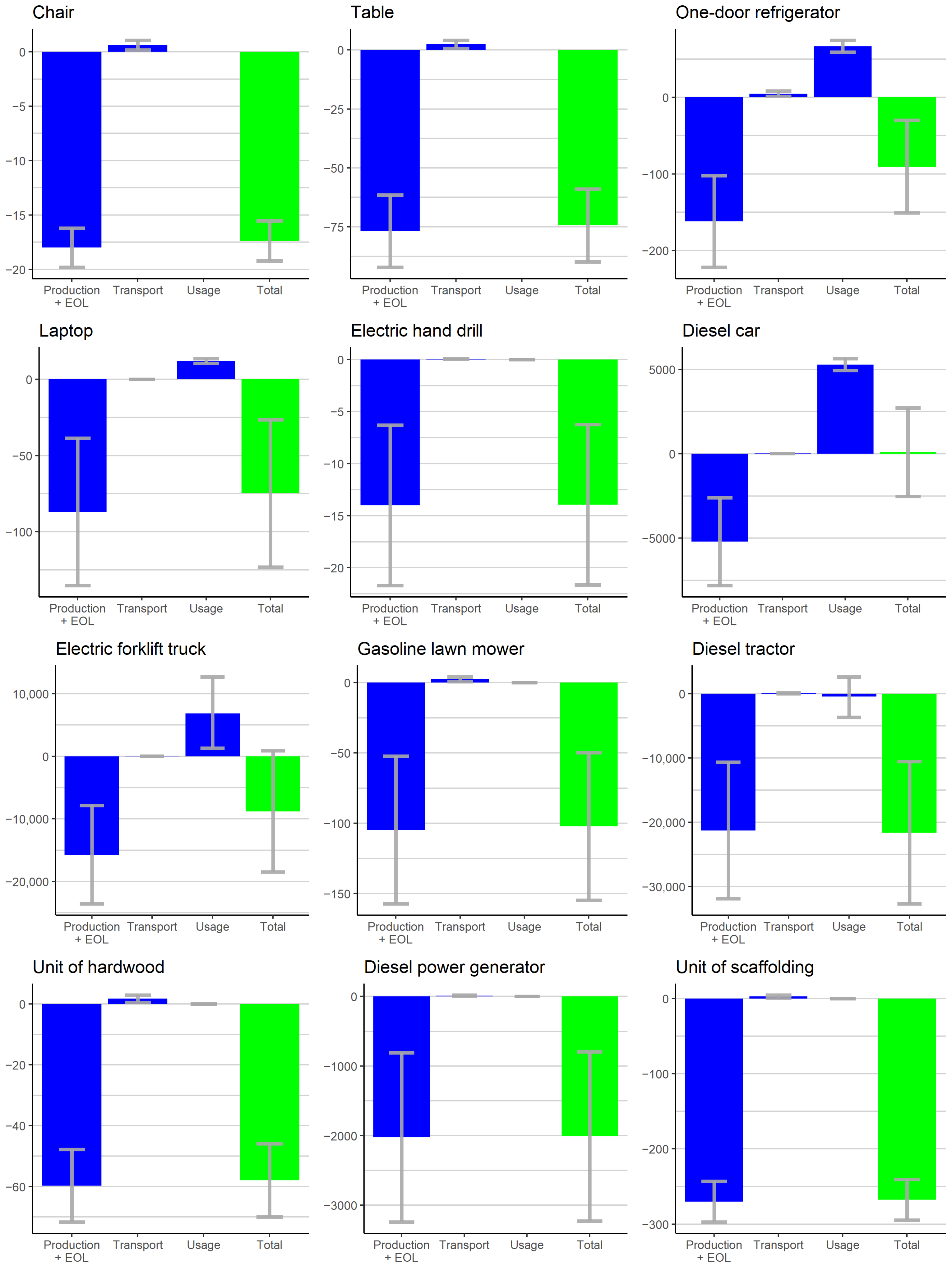
4.1. Effects of Typical Lots on GHGs

The results of the calculations on typical single products are shown in Figure 3. These results are about the residual lifetimes of the goods. The vertical axes display the impact on GHG emissions in kilograms of CO_2e. Bars with negative values mean that GHGs are saved and those with positive values mean that additional GHGs are emitted due to the transaction and utilization of a used good. Note that the vertical axes of the different product types have different scales. The blue bars correspond to components of the life cycle and the green bars are the sum of those blue bars. The uncertainty ranges, such as discussed in Section 3.2, are in gray.

When the displacement rate is 1, which means that reusing is compared to purchasing new, and lot and travel characteristics are fixed, secondhand trade has a beneficial impact on GHGs, with 95% certainty for all product types except for cars and forklift trucks. Transportation emissions are relatively small in all cases. It is also noteworthy that emission savings are on the order of tonnes of CO_2e for vehicles and power generators only, and that the uncertainty ranges are usually very large, especially for powered goods.

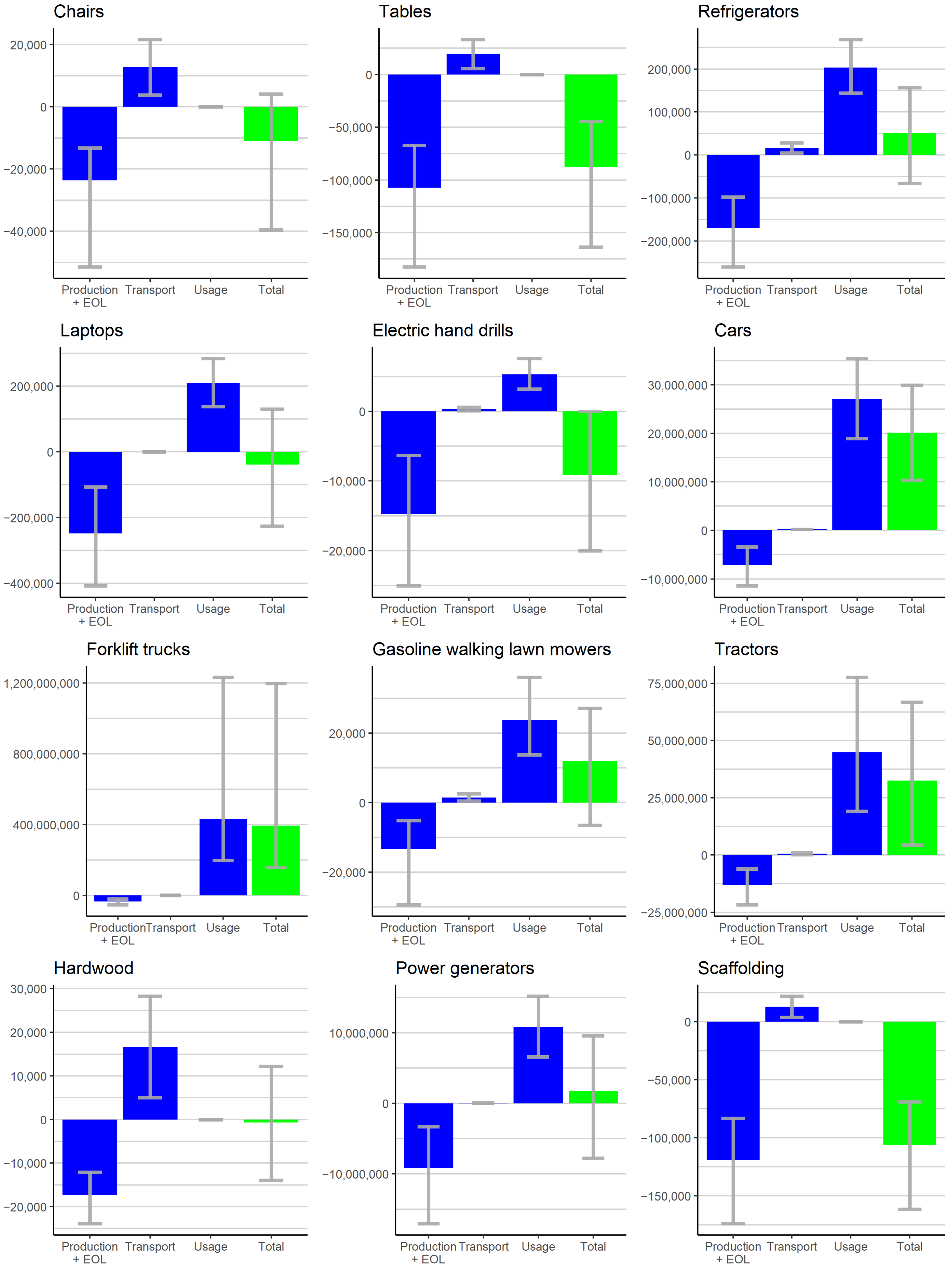
4.2. Residual Lifetime Models

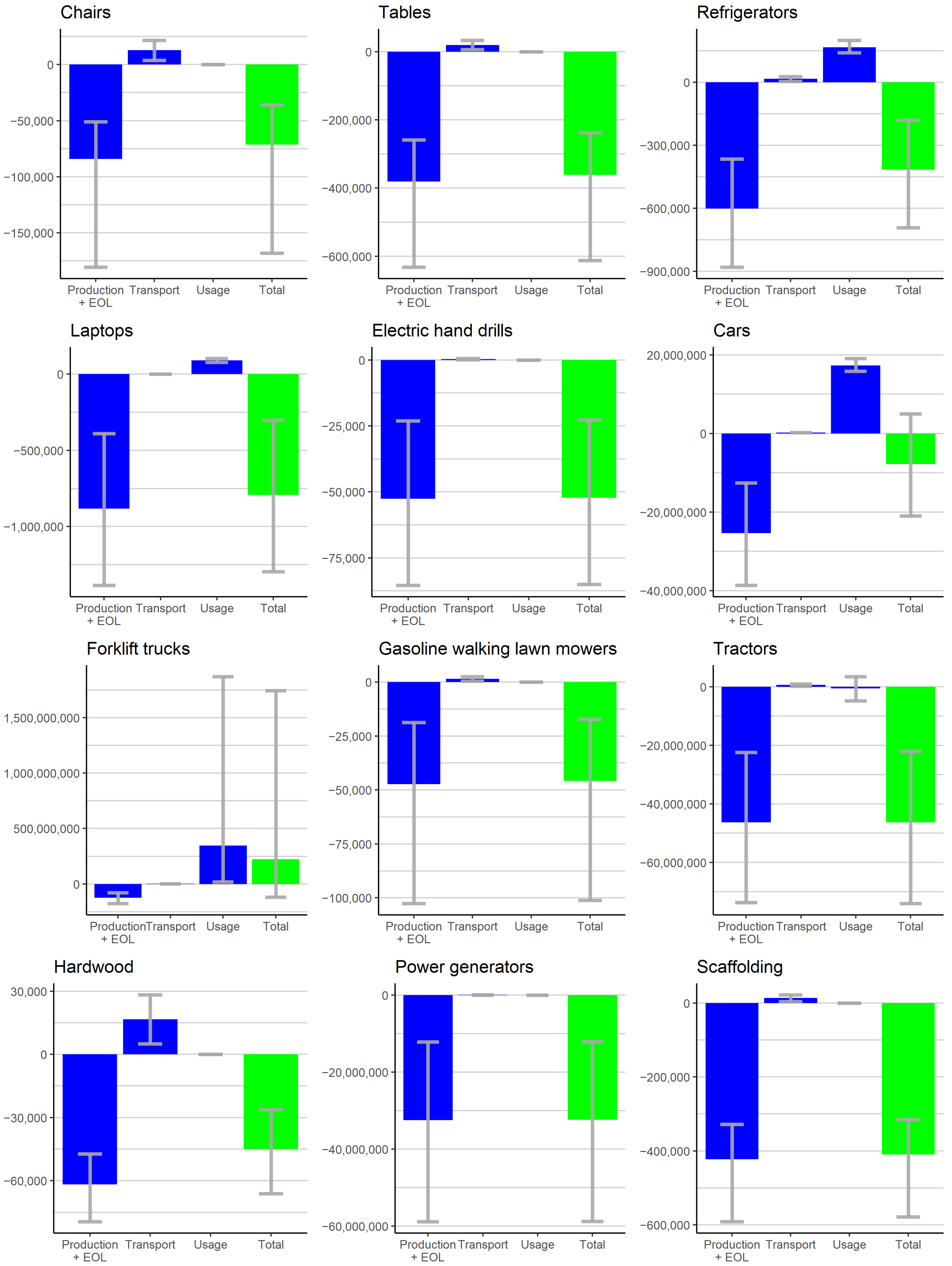
The model of Equation (5) was estimated and some tests were performed. After homoskedasticity was accepted after a Breusch-Pagan test, the model did not pass a Ramsey RESET with two terms to check its functional form. It did after a cross term was added, while adding squared variables did not change it. The results of this model are in

Table 5. Results of the model of Equation (5). The dependent variable is the residual lifetime ($ln(r_i+1)$). $R^2=0.046$.

	Estimate	Std. Error	p-Value
${\beta }_0$: Intercept	4.870	1.134	0.000
${\beta }_1$: Age ($ln(a_i+1)$)	−1.761	0.600	0.004
${\beta }_2$: Lifespans ($ln(\mathbb{E}\left(l_i\right)$)	−1.133	0.481	0.020
Age × lifespans	0.696	0.246	0.005

. The predictive power of the model is low ($R^2=4.6\%$).

Normality of the residuals was rejected after a Jarque-Bera test, as the tails of their distribution were too fat. The Jarque-Bera test was also used to test for other distributions, namely the Cauchy distribution and the logistic distribution. This can be done by transforming the residuals from the hypothesized distribution to the normal distribution and then using the Jarque-Bera test again. With this method, the logistic distribution was accepted. This distribution will be used to simulate predictions about residual lifetimes of Troostwijk lots. No outliers were found when an outlier was defined as an observation whose dummy variable would be statistically significant at a 5% level with a Bonferroni correction.

The model of Equation (6) had no heteroskedastic errors and the functional form was not incorrectly specified. The results are in

Table 6. Results of the model of Equation (6). The dependent variable is the residual lifetime ($ln(r_i+1)$). $R^2=0.025$.

	Estimate	Std. Error	p-Value
${\beta }_0$: Intercept	2.535	0.308	0.000
${\beta }_1$: Age ($a_i$)	0.076	0.034	0.028
${\beta }_2$: Lifespans ($\mathbb{E}\left(l_i\right)$)	−0.045	0.027	0.096
${\beta }_3$: Age/lifespans	−0.828	0.377	0.029

. The predictive power of this model is again low ($R^2=2.5\%$). Again, no outliers were found and the residuals seem to have a logistic distribution.

The model with the highest predicting power was chosen, which is the model of Equation (5) and Table 5. Its results imply that older products are used for a shorter time, but that this effect decreases as lifespans increase. This part sounds intuitive, but the significantly negative sign of the lifespans variable is counterintuitive.

4.3. Sums of Lots

The step of calculating summed environmental impacts consists of adding up the outcomes of Equation (3) per product group using the predictions described above in Section 4.2, among others. The estimates for the displacement rates are $D{R}_{\mathrm{new}}=28.1\%$ (between $22.1\%$ and $35.0\%$) and $D{R}_{\mathrm{used}}=47.7\%$ (between $40.1\%$ and $54.9\%$). This is comparable to the study by Erdmann [2]. Of the respondents in that study that did not reply ’Other’ or ’I cannot answer’, 31.1% reported that they displaced a new good and 49.5% that they displaced a used good.

The results of the calculations, extrapolated to all lots of the different product types and with the displacement rates discussed above, are shown graphically in Figure 4. Now only tables, hand drills and scaffolds have a desirable impact on GHG emissions. Trading used vehicles, i.e., cars, forklift trucks and tractors, is now associated with an increase in emissions. The other product types do not have an effect on GHG emissions that is good or bad with 95% certainty. The difference with Figure 3 seems to be due to the low displacement rates for new products, combined with significant usage or transportation emissions. Transportation emissions increased as a significant share of sales are international. This implies that the net effects of secondhand trade in chairs and hardwood are ambiguous only because transport emissions are included in Formula (3). Averages per product type can be found in

Table A1. Average additional emissions per product type at Troostwijk Auctions in kg CO_2e.

	Chair	Table	Refrigerator	Laptop
Lower bound	−11.65	−81.72	−43.82	−74.47
Expectation	−3.22	−43.83	34.33	−12.81
Upper bound	1.20	−22.25	104.88	42.89
	Hand drill	Car	Forklift truck	Lawn mower
Lower bound	−12.94	3663.84	49,704.09	−41.79
Expectation	−5.89	7147.77	124,614.02	76.75
Upper bound	−0.00	10,608.52	377,981.80	175.21
	Tractor	Hardwood	Power generator	Scaffolding
Lower bound	4342.88	−6.40	−5103.46	−216.10
Expectation	31,986.53	−0.33	1148.31	−141.91
Upper bound	65,655.70	5.59	6292.19	−92.11

in Appendix B. The results of the same calculation when $D{R}_{\mathrm{new}}=1$ and $D{R}_{\mathrm{used}}=0$, so when each used good replaces a new one, are displayed in Figure A1. Averages can be found in

Table A2. Average additional emissions per product type at Troostwijk Auctions in kg CO_2e, if the displacement rate for new goods is assumed to be one.

	Chair	Table	Refrigerator	Laptop
Lower bound	−49.53	−306.00	−464.67	−425.69
Expectation	−21.04	−180.77	−279.53	−260.69
Upper bound	−10.60	−118.87	−121.05	−99.06
	Hand drill	Car	Forklift truck	Lawn mower
Lower bound	−54.98	−7450.89	−37,822.54	−652.30
Expectation	−33.76	−2775.76	69,972.78	−295.93
Upper bound	−14.70	1766.14	550,504.55	−111.46
	Tractor	Hardwood	Power generator	Scaffolding
Lower bound	−72,840.91	−30.30	−38,561.82	−773.72
Expectation	−45,637.64	−20.66	−21,274.70	−548.72
Upper bound	−21,781.11	−12.06	−7918.60	−421.38

.

The assumption of this calculation is that every lot in a product category is indeed of the correct product type. This does not have to be true, lots in the dataset can incidentally also be parts of this product or complements to this product. For example, the battery of a forklift truck can also be classified in the Forklift trucks category. For the same reason of misleading lot names, garages were excluded from the analysis except from the regression in Section 3.9, although it was originally planned to analyze them.

Moreover, it is possible that not all lots containing two or more goods were correctly filtered out. Thus, one should be cautious interpreting these results.

5. Discussion

5.1. Summary of Findings

This paper attempted to identify the sustainability of secondhand markets in terms of GHGs. Four-wheel drive tractors, lawn mowers, scaffolding, catering (’horeca’) refrigerators, restaurant tables, power generators, electric hand drills, laptops, dining chairs, forklift trucks, cars, and hardwood were studied. Various sources were combined to propose a formula and to find values for the parameters. Several regressions also helped filling in those parameters. Uncertainty was handled using Monte Carlo simulation. It appears that it is very important whether or not one assumes that new goods are displaced by used goods one-to-one. A survey was sent out to the buyers of the goods that were studied to test this assumption. From this survey, it appeared that about 28% of the buyers would otherwise have purchased a new good. This might imply that used goods are used as complements of rather than substitutes for new goods.

In a first analysis about lots with average characteristics, it has become clear that the avoided manufacturing and EoL emissions of displaced new goods dominate over transportation and usage emissions. This means that the net effect on GHG emissions is negative with 95% certainty for ten of the twelve product types studied.

In a more general analysis, where the assumptions on the characteristics of the typical product were abandoned, uncertainty has grown. This is partially due to the uncertainty predicting the residual lifetime of goods. The model that is used to predict this does find statistically significant correlations, but has almost no predictive power.

The results are in favor of reusing products, or neutral about it at worst, when reusing is compared to buying new products, so when the displacement rate for new goods ($D{R}_{\mathrm{new}}$) equals 1. This completely changes when the displacement rates for new and used goods ($D{R}_{\mathrm{new}}$ and $D{R}_{\mathrm{used}}$) from the survey results are used. Then, reusing is often neutral, and even bad in the case of vehicles.

The research question was: What are the external effects of an online business-to-business marketplace due to GHG emissions? It seems safe to conclude that these marketplaces allow for a reduction of emissions, when the users buy used goods that they would otherwise have bought new and when they do not use the saved money for additional polluting purchases. This does, however, not mean that emissions are actually saved, because these marketplaces can lead to increased consumption.

5.2. Comparison with Existing Literature

This paper is, to the authors’ best knowledge, one of few papers that assessed the sustainability of secondhand trade by focusing on a specific marketplace. The analysis has been carried out as completely as possible. Many aspects were discussed and quantified. Energy inefficiency of older products, transportation emissions and the displacement rates of other goods were all included. This makes this paper rather complete. An integral part of this study consisted of finding the uncertainty and distributions of parameters in the model. This means that the impact of the assumptions made on estimates is not too big.

The environmental effects of reusing compared to buying new in this study are comparable to those found by Snijder et al. [12] and Erdmann [2]. However, as opposed to the results of Erdmann [2], the results do not imply that powered goods with large carbon footprints cause an increase in emissions. According to the present study, resales of refrigerators, tractors and power generators save emissions compared to new purchases. Fuel-powered products were not included by Erdmann [2], and it is not clear whether he would classify refrigerators as powered goods with large carbon footprints.

This study finds that the environmental benefits of reusing decrease when reported data on product displacement rates are used. This rebound to the emission savings of secondhand markets is consistent with the literature on displacement rates.

5.3. Implications for Policy and Practice

The main purpose of this study is to allow insight into the environmental effects of secondhand trade. This can be of use to all kinds of economic actors. For example, the importance of the displacement rate is useful. For the private sector, these results imply that platforms trading in used goods should aim at the right kind of buyer. If a platform or store manages to attract buyers that were planning to purchase a new product or that were at least seriously considering that, the displacement rate might increase. This means that the results in Figure 4 would change to those in Figure A1. Additionally, governments should take into account the effect of their policy on the displacement rate when designing policy, and consumers can choose not to purchase a used good when they were not considering buying a new one.

Another use for the results of this study is that it allows companies trading in used goods to concentrate on those product categories with the best environmental impact. Assuming Figure 4, firms minimizing their environmental footprint could choose not to expand their trade in vehicles, for example.

5.4. Limitations

Databases with carbon footprints of all kinds of goods are scarce. The Base Carbone database by ADEME has its limitations such as its focus on France, its limited size, and the need to look into documentation, often in French, to find more details on carbon footprints. Moreover, annual efficiency improvements had to be based on scientific literature.

Only environmental effects were taken into account in this paper, even though secondhand markets are of interest for a wide range of disciplines [4]. The environmental effects can differ from the social effects, among others. For example, although additional consumption is bad from an environmental perspective, it is desirable for social welfare and participation [2,14]. This is illustrated by the additional vehicle ownership due to secondhand trade that was observed in Mexico and that increased emissions [18]. Nonetheless, it would be harsh to condem this development as it merely lowers the difference between consumption levels in Mexico and those in developed countries. Such considerations are, however, outside the scope of this paper.

Environmental sustainability and external effects of secondhand markets are very broad notions. This paper only focuses on the effect on global warming. There are, however, many other environmental threats besides global warming. These include, but are not limited to, scarcity of natural resources [11], toxic emissions that do not contribute to global warming, for example in landfills [17], and water usage [10]. The sign and the relative magnitude of the impact that secondhand trade has on some of these threats may resemble the impact on GHG emissions. This may be different for other threats, for example because one aspect of the life cycle is particularly important for that environmental threat. For instance, secondhand trade probably influences natural resource depletion in a desirable way. This claim will only be false when older vehicles need a huge amount of materials for repairs, which should not be left out of consideration [41].

A lot of information is uncertain or scarce. Often, estimations are approximate rather than actually reliable. This causes uncertainty ranges to be so large, that few meaningful conclusions can be drawn from the calculations in this paper. Large uncertainty is a known issue for LCAs [7,25]. Two considerations regarding imperfect or uncertain data have not been discussed yet. Firstly, because of inconsistent carbon footprint estimates, vans were excluded from the analysis except from the regression in Section 3.9. Vans were originally planned to form an additional product type in this case study. Secondly, one could question the assumption that the efficiency change c did not have uncertainty ranges for product types for which it was assumed to be 0.

Uncertainty about the distances of transportation was not included. The distances used, based on geodesic distances between major cities in the country of origin and of destination, are probably inaccurate. Sometimes they will be too short, since actual routes are not as short as geodesic distances. They will be too big in other cases, since buyers will probably bid on lots that are close to their homes and that are not located at random in the country of origin. There were also no assumptions made on transportation distances of used goods that are traded through other channels.

Additionally, not all lots other than cars will be transported by trucks. They might also be transported with a ship or driven by car or van. It was assumed that cars drove themselves to their destination, but this assumption ignores the fact that buyers will often need transport to the pick-up location. However, the transportation component is so marginal for cars according to all calculations, that doubling or even tripling transport emissions changes little.

There is reason to believe that the results about forklift trucks are unrealistic, since the assumption of 2000 operating hours per year implies that a forklift truck is operated every working hour in the year. In practice, forklift trucks can also stand by and be used a part of the time only. However, no empirical estimates on annual operating hours of forklift trucks were found.

Two more technical limitations are about the distributions that are assumed for empirical data. In this paper, the logistic and loglogistic distributions were used at various points because they fit the data better than the normal and lognormal distributions. Some would argue that these distributions should only be used when they fit the data not only empirically, but also theoretically.

Finding the distribution of the share of a new good’s lifespan that is displaced by a used good, i.e., the distribution of r/l, gives unexpected results. The expectation of this ratio becomes far higher than one would intuitively guess, so that used goods are expected to be used longer than new goods. An additional model such as Equations (5) and (6) but where r/l is estimated immediately might function better than first estimating r and then dividing that estimate by l. Another alternative is assuming a Weibull distribution conditional on the current age of a lot rather than using survey data.

Finally, this paper implicitly assumes that all environmental gains or losses could be attributed to the online auction platform. However, there are also a buyer and a seller involved that could be assumed responsible for these environmental impacts. This is especially important because the desirability of trade in used goods depends on whether the buyer uses it in addition to or instead of new goods.

5.5. Recommendations for Further Research

The displacement rates $D{R}_{\mathrm{new}}$ and $D{R}_{\mathrm{used}}$ were very important for the conclusions of this paper. However, the way that they were derived was rather simplistic. More founded research on these displacement rates should be included in future analyses such as this one. Price elasticities could be calculated, such as Zink et al. [13] do. A comprehensive analysis should also account for the possibility that used goods can displace goods of other product types. Lastly, future research could try to relax the assumption of the demand-constrained market.

Future research with access to many respondents can try to improve the reliability of survey data. For example, research can control for demographic factors. Additionally, it can use Likert scales or implement techniques such as conjoint analysis to control for social desirability bias. It will be a methodological challenge to convert findings based on methods like the latter to displacement rates.

As mentioned, the model to predict the residual lifetimes of goods left much to be desired. Models with higher predicting power should be developed in the future. Those models might not have the seemingly unrealistic values of $\mathbb{E}(r/l)$ that were discussed in Section 5.4, if they are designed properly.

There is much more data available on carbon footprints and on annual efficiency improvements of consumption goods such as laptops and refrigerators than on production goods such as forklift trucks and power generators. This indicates that there is a field to be explored by new LCAs.

The final recommendation for researchers on specific marketplaces is to interview people to get the information that is scarce but so important. A researcher could go to a pick-up location of lots and see whether buyers are willing to answer some questions. These questions could be comparable to the ones now asked in the survey, for example about how old the lot is and for how long it is expected to be used. Moreover, they could ask how far the buyers have to travel, what transport mode they are using, and how they are going to spend the money that they may have saved due to the auction.

References

1. Al-Ghussain, L. Global warming: Review on driving forces and mitigation. Environ. Prog. Sustain. Energy 2019, 38, 13–21. [Google Scholar] [CrossRef] [Green Version]
2. Erdmann, L. Quantifizierung der Umwelteffekte des privaten Gebrauchtwarenhandels am Beispiel von eBay. In Wiederverkaufskultur im Internet: Chancen für Nachhaltigen Konsum am Beispiel von eBay; Behrendt, S., Blättel-Mink, B., Clausen, J., Eds.; Springer: Berlin/Heidelberg, Germany, 2011; pp. 127–158. [Google Scholar]
3. Nearly 3 in 5 Dutch People Used Online Platforms in 2019. Available online: https://web.archive.org/web/20211222150236/https://www.cbs.nl/en-gb/news/2020/14/nearly-3-in-5-dutch-people-used-online-platforms-in-2019 (accessed on 29 November 2021).
4. Hansen, K.T.; Le Zotte, J. Changing Secondhand Economies. Bus. Hist. 2019, 61, 1–16. [Google Scholar] [CrossRef] [Green Version]
5. Fortuna, L.M.; Diyamandoglu, V. Optimization of greenhouse gas emissions in second-hand consumer product recovery through reuse platforms. Waste Manag. 2017, 66, 178–189. [Google Scholar] [CrossRef] [PubMed]
6. Schaubroeck, S.; Schaubroeck, T.; Baustert, P.; Gibon, T.; Benetto, E. When to replace a product to decrease environmental impact?—A consequential LCA framework and case study on car replacement. Int. J. Life Cycle Assess 2020, 25, 1500–1521. [Google Scholar] [CrossRef]
7. Hellweg, S.; Milà i Canals, L. Emerging approaches, challenges and opportunities in life cycle assessment. Science 2014, 344, 1109–1113. [Google Scholar] [CrossRef]
8. Leiserowitz, A.; Maibach, E.; Rosenthal, S.; Kotcher, J.; Bergquist, P.; Ballew, M.; Goldberg, M.; Gustafson, A.; Wang, X. Climate Change in the American Mind: April 2020; Yale Program on Climate Change Communication: New Haven, CT, USA, 2020. [Google Scholar]
9. Bakos, J.; Siu, M.; Orengo, A.; Kasiri, N. An analysis of environmental sustainability in small & medium-sized enterprises: Patterns and trends. Bus. Strategy Environ. 2020, 29, 1285–1296. [Google Scholar]
10. Cooper, D.R.; Gutowski, T.G. The Environmental Impacts of Reuse: A Review. J. Ind. Ecol. 2017, 21, 38–56. [Google Scholar] [CrossRef]
11. Bakker, C.; Wang, F.; Huisman, J.; Den Hollander, M. Products that go round: Exploring product life extension through design. J. Clean. Prod. 2014, 69, 10–16. [Google Scholar] [CrossRef]
12. Snijder, L.; Broeren, M.; Bergsma, G. The Environmental Benefit of Marktplaats Trading; CE Delft: Delft, The Netherlands, 2019. [Google Scholar]
13. Zink, T.; Geyer, R.; Startz, R. A Market-Based Framework for Quantifying Displaced Production from Recycling or Reuse. J. Ind. Ecol. 2015, 20, 719–729. [Google Scholar] [CrossRef]
14. Thomas, V.M. Demand and Dematerialization Impacts of Second-Hand Markets: Reuse or More Use? J. Ind. Ecol. 2003, 7, 65–78. [Google Scholar] [CrossRef]
15. Craglia, M.; Cullen, J. Do technical improvements lead to real efficiency gains? Disaggregating changes in transport energy intensity. Energy Policy 2019, 134, 110991. [Google Scholar] [CrossRef]
16. Diaz, L.F. Waste management in developing countries and the circular economy. Waste Manag. Res. 2017, 35, 1–2. [Google Scholar] [CrossRef] [PubMed]
17. Yoshida, A.; Terazono, A. Reuse of secondhand TVs exported from Japan to the Philippines. Waste Manage. 2010, 30, 1063–1072. [Google Scholar] [CrossRef] [PubMed]
18. Davis, L.W.; Kahn, M.E. International Trade in Used Vehicles: The Environmental Consequences of NAFTA. Am. Econ. J. Econ. Policy 2010, 2, 58–82. [Google Scholar] [CrossRef] [Green Version]
19. IPCC. Climate Change 2014: Synthesis Report; IPCC: Geneva, Switzerland, 2014. [Google Scholar]
20. ADEME. Documentation des Facteurs d’Émissions de la Base Carbone; ADEME: Angers, France, 2020. [Google Scholar]
21. Wang, P.; Deng, X.; Zhou, H.; Yu, S. Estimates of the social cost of carbon: A review based on meta-analysis. J. Clean. Prod. 2019, 209, 1494–1507. [Google Scholar] [CrossRef]
22. De Koning, A.; Schowanek, D.; Dewaele, J.; Weisbrod, A.; Guinée, J. Uncertainties in a carbon footprint model for detergents; quantifying the confidence in a comparative result. Int. J. Life Cycle Assess. 2010, 15, 79–89. [Google Scholar] [CrossRef] [Green Version]
23. Lenzen, M.; Wood, R.; Wiedmann, T. Uncertainty analysis for multi-region input–output models—A case study of the UK’s carbon footprint. Econ. Syst. Res. 2010, 22, 43–63. [Google Scholar] [CrossRef]
24. Mattila, T.; Kujanpää, M.; Dahlbo, H.; Soukka, R.; Myllymaa, T. Uncertainty and Sensitivity in the Carbon Footprint of Shopping Bags. J. Ind. Ecol. 2011, 15, 217–227. [Google Scholar] [CrossRef]
25. Igos, E.; Benetto, E.; Meyer, R.; Baustert, P.; Othoniel, B. How to treat uncertainties in life cycle assessment studies? Int. J. Life Cycle Assess 2019, 24, 794–807. [Google Scholar] [CrossRef]
26. Crowder, S.; Delker, C.; Forrest, E.; Martin, N. Introduction to Statistics in Metrology; Springer: Cham, Switzerland, 2020. [Google Scholar]
27. Lee, S.H.; Chen, W. A comparative study of uncertainty propagation methods for black-box-type problems. Struct. Multidiscipl. Optim. 2009, 37, 239–253. [Google Scholar] [CrossRef]
28. Mayer, T.; Zignago, S. Notes on CEPII’s Distances Measures: The GeoDist Database; CEPII Working Paper 2011-25; CEPII: Paris, France, 2011. [Google Scholar]
29. View Data. Available online: https://www.bilans-ges.ademe.fr/en/basecarbone/donnees-consulter/choix-reglementation (accessed on 18 November 2021).
30. Non-Road Mobile Machinery Emissions. Available online: https://web.archive.org/web/20211118103828/https://ec.europa.eu/growth/sectors/automotive-industry/environmental-protection/non-road-mobile-machinery_en (accessed on 18 November 2021).
31. ADEME; CIGREF. Technologies Numériques, Information et Communication (TNIC): Guide Sectoriel 2012; ADEME: Angers, France, 2012. [Google Scholar]
32. Li, Q.; Cai, H.; Kelly, J.C.; Dunn, J. Expanded Emission Factors for Agricultural and Mining Equipment in GREET® Full Life-Cycle Model; Argonne National Laboratory: Lemont, IL, USA, 2016. [Google Scholar]
33. Regulation (EU) 2016/1628. Available online: https://web.archive.org/web/20211118104538/https://eur-lex.europa.eu/eli/reg/2016/1628/2020-07-01 (accessed on 18 November 2021).
34. Laleicke, P.F.; Cimino-Hurt, A.; Gardner, D.; Sinha, A. Comparative Carbon Footprint Analysis of Bamboo and Steel Scaffolding. J. Green Build. 2015, 10, 114–126. [Google Scholar] [CrossRef]
35. Energy Consumption in the UK 2021. Available online: https://www.gov.uk/government/statistics/energy-consumption-in-the-uk-2021 (accessed on 18 November 2021).
36. How Long Will an Average Forklift Last? Available online: https://web.archive.org/web/20211118102714/https://www.tmhnc.com/blog/how-long-will-a-forklift-last-and-forklift-average-use (accessed on 18 November 2021).
37. Willems, R.; Molnár-in ‘t Veld, H.; Ligterink, N. Bottom-up Berekening CO2 van Vrachtauto’s en Trekkers; Statistics Netherlands: The Hague, The Netherlands, 2014. [Google Scholar]
38. Kruiskamp, P.; Molnár-in ‘t Veld, H.; Ligterink, N. Bottom-up Berekening CO2 van Bestelauto’s; Statistics Netherlands: The Hague, The Netherlands, 2015. [Google Scholar]
39. ADEME. The Potential of Electric Vehicles; ADEME: Angers, France, 2016. [Google Scholar]
40. Facchini, F.; Mummolo, G.; Mossa, G.; Digiesi, S.; Boenzi, F.; Verriello, R. Minimizing the Carbon Footprint of Material Handling Equipment: Comparison of Electric and LPG Forklifts. J. Ind. Eng. Manag. 2016, 9, 1035–1046. [Google Scholar] [CrossRef] [Green Version]
41. Dyer, J.A.; Desjardins, R.L. Carbon Dioxide Emissions Associated with the Manufacturing of Tractors and Farm Machinery in Canada. Biosyst. Eng. 2006, 93, 107–118. [Google Scholar] [CrossRef]
42. Test Report Search—Tractor Test Lab. Available online: https://tractortestlab.unl.edu/test-page-nttl (accessed on 5 October 2021).
43. Lhotellier, J.; Less, E.; Bossanne, E.; Pesnel, S. Modélisation et Évaluation ACV de Produits de Consommation et Biens d’Équipement: Rapport; ADEME: Angers, France, 2018. [Google Scholar]
44. Lhotellier, J. Modélisation et Évaluation Environnementale de Produits de Consommation et biens d’Équipement: Rapport; ADEME: Angers, France, 2019. [Google Scholar]
45. Mak, W.M. Environmental Externalities of Secondhand Markets: Based on a Dutch Auctioning Company. Master’s Thesis, Vrije Universiteit, Amsterdam, The Netherlands, 2 July 2021. [Google Scholar]
46. Association Bilan Carbone. Methodological Guidelines: Appendices; Association Bilan Carbone: Paris, France, 2017. [Google Scholar]
47. Michel, A.; Attali, S.; Bush, E. Energy Efficiency of White Goods in Europe: Monitoring the Market with Sales Data; ADEME: Angers, France, 2016. [Google Scholar]
48. Murakami, S.; Oguchi, M.; Tasaki, T.; Daigo, I.; Hashimoto, S. Lifespan of Commodities, Part I: The Creation of a Database and Its Review. J. Ind. Ecol. 2010, 14, 598–612. [Google Scholar] [CrossRef]
49. Lifespan Database for Vehicles, Equipment, and Structures: LiVES. Available online: http://www.nies.go.jp/lifespan/index-e.html (accessed on 5 October 2021).
50. Gonçalves, D.N.; de Morais Gonçalves, C.; de Assis, T.F.; da Silva, M.A. Analysis of the difference between the Euclidean distance and the actual road distance in Brazil. Transp. Res. Procedia 2014, 3, 876–885. [Google Scholar] [CrossRef] [Green Version]
51. Meyerding, S.G.H. Job preferences of agricultural students in Germany: A choice-based conjoint analysis for both genders. Int. Food Agribusiness Manag. Rev. 2018, 21, 219–236. [Google Scholar] [CrossRef]
52. Gao, Z.; Hu, Q.; Xu, X.; Wang, W. Residual Lifetime Prediction with Multistage Stochastic Degradation for Equipment. Complexity 2020, 2020, 8847703. [Google Scholar] [CrossRef]
53. Lin, G.D.; Hu, C. On characterizations of the logistic distribution. J. Stat. Plan. Inference 2008, 138, 1147–1156. [Google Scholar] [CrossRef]
54. Wood Density and Hardness. Available online: https://web.archive.org/web/20210310052523/https://qtimber.daf.qld.gov.au/guides/wood-density-and-hardness (accessed on 18 November 2021).
Figure 1. Overview of the calculation of the environmental impact of online auctions.
Sustainability 14 01682 g001
Figure 2. Annual efficiency of laptops, refrigerators, 4-wheel drive tractors, and cars, with the R 2 (R-squared) statistics. These goods consume 2.57% (laptops), 3.85% (refrigerators), −0.02% (tractors) and 1.43% (cars) more energy per year that they are older.
Sustainability 14 01682 g002
Figure 3. Carbon footprint (kg CO2e) of reselling goods with the characteristics from Table 2, when D R new = 1 . 95% uncertainty ranges are in gray.
Sustainability 14 01682 g003
Figure 4. Carbon footprint (kg CO2e) of reselling all goods of their product types (summed). 95% uncertainty ranges are in gray. See step 2 in Section 3.10 for the difference between this figure and Figure 3.
Sustainability 14 01682 g004