Abstract
Construction costs and investment planning are the decisions made by construction managers and financial managers. Investment in construction materials, labor, and other miscellaneous should consider their huge costs. For these reasons, this research focused on analyzing construction costs from the point of adopting multivariate cost prediction models in predicting construction cost index (CCI) and other independent variables from September 2021 to December 2022. The United States was selected as the focal country for the study because of its size and influence. Specifically, we used the Statistical Package for Social Sciences (SPSS) software and R-programming applications to forecast the elected variables based on the literature review. These forecasted values were compared to the CCI using Pearson correlations to assess influencing factors. The results indicated that the ARIMA model is the best forecasting model since it has the highest model-fit correlation. Additionally, the number of building permits issued, the consumer price index, the amount of money supply in the country, the producer price index, and the import price index are the influencing factors of investments decisions in short to medium ranges. This result provides insights to managers and cost planners in determining the best model to adopt. The improved accuracies of the influencing factors will help to enhance the control, competitiveness, and capability of futuristic decision-making of the cost of materials and labor in the construction industry.
1. Introduction
Construction involves tremendous investment in labor, machinery, capital, and other external support. One of the important decisions to make during construction is how to invest and what to invest in. Researchers noticed actual public construction costs are mostly higher than the expected or budgeted costs [1,2]. For example, 61.89% of government works constructed between 2006 and 2017 in Brazil had cost inflated by the end of the projects [3]. In this case, cost overrun refers to the situation that the expenditure of a project exceeds its calculated budget [4]. There is no unanimous decision or explanation on why cost overrun happens, but it often originates from the planning stage of the project. Added costs (not budgeted for) can affect project performance and time because cost, time, and schedule are the triple constraints of every project. Therefore, any change in one variable affects the performance of the other two variables. For instance, an increase in the cost of a project will affect the completion time when extra monetary commitments are beyond the budget to accommodate inflation. This change in construction cost can also impact the schedule by limiting the scope of work (to complete) because of the cost implications of unable to meet the increase in the construction cost. This issue affects many nations such as Portugal, Ghana, China, and Indonesia [4,5]. Cost estimation is particularly important especially when tight restrictions exist on construction budgets [6]. Estimating or predicting costs within an acceptable margin of error can help curb these challenges in cost budgeting [7]. Therefore, construction companies need accurate and practical methods to analyze construction costs.
Researchers have explored varied methods to simplify the complexity of cost predictions caused by consistent overruns. One approach is to forecast costs using the Construction Cost Index (CCI), whose calculations involve certain hours of common labor (e.g., 200) and the prices of a few representative construction materials (e.g., steel, concrete, and lumber) from 20 cities sampled in the U.S. Both private and public agencies in construction investment adopt the CCI for decision making. Additionally, field research is also a way of gathering data for cost prediction [8]. The prediction methods include the Simple Moving Average (SMA), the Exponential Smoothing (ES), and the Autoregressive Integrated and Moving Average (ARIMA). However, these methods still need improvement since they have significant margins of error [9]. Artificial Neural Network (ANN) can help to understand and predict construction costs using realistic estimated values [10,11]. During the initiation stage of a project, several computation models such as Support Vector Machines (SVM) and ANN are capable to improve prediction accuracy [12]. According to [6], other researchers like [13] explored Vector Error Correction models, while [14] adopted genetic algorithms. In estimating practice, project managers analyze the rate per unit cost of a floor area to predict the construction costs [15]. However, managers are unsure which method can provide the most reliable analysis and predictions on the labor and material costs of construction projects.
This research aims to help managers to find and analyze the influencing factors of construction cost prediction to make good decisions. Since construction budgeting happens at the initiation stage, these factors are critical because any misinformation could lead to poor project decisions. Researchers have not yet agreed on the exact models of influencing factors for the prediction of construction cost overruns. While some discussed the subject of cost overrun in general, others could not supply substantial information on how construction cost overruns occur since many factors affect a construction project’s performance other than cost. This pending problem has ignited the concerns of stakeholders on how to accurately predict construction costs. Hence, this research targets the following hypotheses: H0—There are no major influencing factors for the prediction of construction cost overruns; H1—Major influencing factors for the prediction of construction cost overruns exist. This paper is expected to contribute to the accuracy of construction cost predictions. Specifically, the paper reviews and compares the influence factors and the prediction methods to establish an improved cost estimation and investment planning strategy. The goal is to establish a scheme for the construction industry to consider when planning actions designed to achieve their long-term or overall aim of development.
The research design combines the influencing factors retrieved from the literature review and the multivariate analysis variables of construction cost indexes gathered from the Engineering News Records (ENR). The selection of the factor analysis method is based on the comparison of the prevailing prediction methods for accuracy and practicability. Through the data analysis, the discussion presents the trend of CCI using descriptive analysis and Pearson Correlation. Then, the paper provides the forecasts of CCI using Holt Model and generates R-squared coefficients and mean average percentage errors (MAPEs). The paper also analyzes the Pearson Correlations of forecasted and original independent variables, and their impacts of transportation metrics on the CCI. The results reveal the current trend of the construction industry and the influences of the transportation delays that the world is experiencing. The outcomes of this research also include the selection of variables based on the literature review, their influencing factors, industry trends, and reliable prediction models.
The next section of this paper will examine and compare the published articles of the calculations and predictions of construction costs. It also includes the discussion of relevant knowledge gaps. This section will highlight the proposed solution and explain the method of this research. Section 3 presents the results and discussions, which include the trend of CCI, descriptive analysis, forecast of CCI and independent variables, Pearson Correlations, impacts of transportation metrics, and forecast of transportation indicators. Section 4 includes the conclusion and suggestions for further studies. It sheds light on the workings of the influencing factors of construction cost and project planning.
2. Materials and Methods
Construction practitioners challenged the historical CCI (see Equations (1)–(4)) because of the short variations that exist in CCI predictions [16]. They explained that fluctuation in the CCI makes it difficult to accurately predict labor and material costs for construction decision-making. There are two traditional methods for forecasting the CCI. The casual method forecasts construction costs are based on independent explanatory variables whilst the time series forecasts cost based on the records and related variations. Additionally, the time series method was chosen where the data was from January 1975 to December 2008, summing up to 408 points. The research compared data of the ENR against prediction models such as the Simple Moving Average (SMA), Holt ES, Holt-winters, Autoregressive Integrated Moving Average (ARIMA), and Seasonal ARIMA. All the models have some accuracy, though the ARIMA and seasonal ARIMA have the highest accuracy index. However, CCI was exact in mid-and long-term forecasts [17]. The current time-series methods were imprecise in predicting or forecasting for mid to long time forecasting. The researchers selected input variables through the collection of raw data from the US Bureau of Labor Statistics and the ENR. They applied machine learning algorithms such as the k-nearest neighbor algorithm (K-NN) model training and testing, and the part model training and testing to generate predicted results. They then compared various models, such as the Mean Absolute Percentage Error (MAPE, see Equation (5)), Mean Squared Error (MSE, see Equation (6)), and Mean Absolute Error (MAE, see Equation (7)), to measure the accuracy. They also compared the predicted assessments generated from the K-NN model to the real CCI sourced from the ENR monthly publications and repeated the comparisons for the mid-term of 60 months and the long-term of 84 months respectively. Their results showed that prediction errors in time series models increase when considering longer time.
The cwt stands for one hundredweight (abbreviated as CWT) is a standard unit of weight or mass used in certain commodities markets. The is the number of fitted points, is the actual value, is the forecast value, and Σ is the summation of the forecasted values for the period under consideration. As the name suggests, the MAPE indicates the reliability of the predicted values or the percentage error of the mean values. Furthermore, the factors to consider when selecting an index include the purpose of the index, selection of cost elements, choice of weights of each element, and choice of a base year [12]. Particularly, historical CCIs were collected from the United States Central Agency for Public Mobilization and Statistics, and generated forecast prices for the Neural Networks, Regression Method, and Autoregression time series different models. They were then analyzed and compared for the performances of the three models. The findings of [12] showed that the autoregressive time series has the least absolute errors of 3.5. The regression method had the most absolute errors of 17.5 and was, therefore, the least effective method. According to [13,18], one reason for the errors in CCI predictions was the use of only univariate analysis in the estimation. The researchers listed several multi-variables that were determinants in forecasting construction costs. These include consumer price indexes, employment level in construction, building permits, money supply, crude oil, prices, producer price index, and housing start dates. The sources of the variables were from areas such as the U.S. Bureau of Labor Statistics, the U.S. Bureau of Census, the Board of Governors of the Federal Reserve Systems, and the U.S. Bureau of Economic Analysis. Moreover, the researchers conducted the unit root test and the Granger Causality Test to decide the ranking of the variables and the usefulness of one variable in predicting another variable, respectively. The research concluded that there was no single multivariable time-series analysis or model in forecasting construction costs.
Artificial Intelligence is helpful to CCI analysis. Researchers [19] also expressed that using a single ANN method was flawed because its analysis had biases. The researchers, therefore, proposed an ensemble model comprising of one average and two stacked generalizations. They concluded that the use of an ensemble of the neural network is more precise than the use of a single ANN model for construction costs predictions. For example, Tarmizi et al. [20] reviewed external influencing factors of construction cost indexes. The study was carried out in Sumatra in Indonesia where data was collected from twenty-five cities in North Sumatra. The corresponding data collection was on the economic growth of the cities, the impact of duty on land acquisition, and the construction cost index in those districts. Some of the indicators used to describe the variables were the Annual Domestic Product and the CCI point. They analyzed the impact of economic growth and tax on land acquisition on CCI and found that both the economic growth and the duty on land acquisition affect the construction cost index at least with 95% confidence.
CCI values are subject to significant variations [17]. Researchers such as [16] utilized the univariate times series method and concluded that the univariate analysis could only predict in the short term but could not accurately predict long-term construction cost. This was because the error of prediction using univariate time series increases over time. To solve this issue, explored multivariate models were developed for effective mid-to-long-term forecasting [13]. On the other hand, traditional methods of forecasting such as the regression methods used in past were not effective because too many independent variables affected the construction costs, and the modern time series approach was rather effective [12].
Furthermore, research conducted by [18] explained that the Autoregressive integrated moving average (ARIMA) was the most effective univariate time-series model, but its statistical relevance could only be applied to short-term forecasting and cannot be used for long-term prediction of construction costs. Moon and Shin [21] explained that the recent construction cost index forecast method that utilizes multivariate analysis provides better results than univariate cost predictions methods though the time of collecting for economic and social information for multivariate analysis may be questionable. Internet search patterns of people can be analyzed with the multivariate analysis to give a more accurate comparison of social and economic indications and CCI. Table 1 shows literature review on influencing factors of cost construction cost prediction as described by previous researchers.
The growth of the construction industry requires precise cost predictions. Many researchers have explored various techniques in predictive costs for decision-making. Construction investment decisions depend largely on the cost predictions, and the accuracy of these predictions affects the outcome of the decisions to be made. Caffieri et al. [22] explore Artificial Neural networks in predicting cost using the construction/building characteristics, such as usage area, average perimeter, building height, etc. This is different from other researchers who have explored different methods. Some of the different methods used include [23]—linear regression, artificial neural network, random forest, and light boosting gradient; [19,20]—Artificial Neural Network; [17]—Machine Learning; [12]—Neural Network, Time-series, and [23,24,25]—BP Neural Network; [13]–Multilayer approach; [18]—Multivariate time-series; [21]—Search Query.

Table 1.
Literature review on independent variable of CCI.
Table 1.
Literature review on independent variable of CCI.
| Factors of Construction Cost Prediction | References | |
|---|---|---|
| Economic growth, Construction cost index | Acquisition of rights to land and building | [20] |
| Types of work (general cost, installation works, engineering works, etc.) Construction side location (in the city center, outside the city center, non-urban, etc.) | The overall duration of the construction works, Size and necessary potential of the main contractor | [19] |
| Consumer price index, employment level in construction, Building permits, Money supply | Crude oil prices, Producer price index Housing starts, Gross domestic product | [18] |
| Consumer price index, Federal funds rate, Unemployment rate, The employment rate in construction, Average weekly hours, Prime loan rate | Building permits, Money supply, Average hourly earnings, Crude oil price, Housing starts, Construction spending, Gross domestic product | [16] |
| The selling price of residential properties, Total transaction of residential properties, | Total number of residences, Total population, Total number of new mortgages | [26] |
| Consumer price index, crude oil price, producer price index, gross domestic product, | employment levels, number of building permits, the number of housings starts the money supply crude oil prices | [27] |
| Payment delay by the client, Change by the client during construction, Owner understanding and granting strategy, Estimator’s experience level, | Estimation methods, Techniques used, Location of project, Quality and contents of specification code | [28] |
| Clear and detailed drawings, Experience and skill level of estimators, Materials (price, availability, quality), Experience on similar projects, | Accuracy of the bill of quantities, Management team, Financial capacity, Quality of assumption, Project complexity of design, | [29] |
Researchers such as [12,17,18,21] have argued that multivariate analysis produces accurate results in forecasting construction costs. The challenge is with the various variables that have been presented. Diverse variables have been proposed by different researchers. Understanding variables that truly impact construction cost prediction is key. There have been disparities in the variables presented by researchers. Tarmizi et al. [20] explained that economic growth and duty on the acquisition of the right to land and building are the variables that affect construction costs, while [19] proposed that the type of works, construction site location, the overall duration of the construction works, and site and necessary potential of the main contractor are the independent factors of construction cost predictions. Tajani [26] on the other hand proposed the selling price of residential properties, total transaction of residential properties, the total number of residences. These are a few of the discrepancies that exist in construction cost estimation enablers. Understanding independent variables in construction cost estimation are very important.
The objective of this study is to examine through literature and multivariate analysis variables of construction cost prediction or indexes. Hence, the research question is, “What are the independent variables of construction cost predictions or indexes?” The researchers adopted the method proposed by [13,18]. The previous authors adopted a multivariate research methodology looking at influencing factors of the Construction Cost Index (CCI). On this basis, it was assumed that the CCI is the dependent variable and the others are independent. The goal of this research is in line with the approach of the previous authors. Nine independent variables were gathered from the literature review. This formed the basis for the data collection. Also, data on the variables were sourced from the following databases: US Bureau of Labor Statistics, Board of Governors of Federal Reserve System, US Bureau of Census, US Bureau of Economic Analysis. Data were collected from January 2019 to August 2021. Also, the CCI from January 2019 to August 2021 from the Engineering News-Record was collected, serving as the dependent variable for the study. Table 2 shows the dependent and independent variables used for the analysis.
Table 2.
List of variables in the study (January 2019–August 2021).
The purpose of the research is to identify independent variables of CCI, thus economic determinants that influence the course of the CCI. Knowing this can inform decision-makers in forecasting what could happen to the construction materials and labor costs based on the changes of these variables. We adopted a two-way analysis approach where the first step provides the Pearson Correlation to identify the variables that have a correction with the CCI. We created a tread line of the CCI to visualize the nature of the CCI from January 2019 to August 2021. We also forecasted the CCI for September 2021 to December 2022 to determine the future trend of the CCI. The adopted Holt Model in this predictive analysis includes the forecast of the identified independent variables from September 2021 to December 2022, and the identified independent variables are also presented. In this research, the analysis compares the Autoregressive Integrated Moving Average method, the Simple Seasonal, and the Winters’ Additives methods using the collected data. The data analysis software is R Programming (version 4.1.2, R Foundation for Statistical Computing, Vienna, Austria) with a combination of the Statistical Package for Social Sciences (SPSS AMOS version 26.0 software, IBM, Armonk, NY, USA). The following section provides the results generated from the analysis.
3. Results and Discussion
3.1. Trend of Construction Cost Index
Figure 1 below shows the trend of the CCI from January 2019 to December 2021. The CCI has been increasing with only a few almost all the times under review. It can be observed that during 2019 the CCI remained stable between March and April, August and September, and November and December. However, the CCI increased steadily throughout the period of 2020, which could be because of the falling economic growth due to the pandemic, therefore, leading to an increase in construction-related variables such as the prices of cement, high labor costs, prices of steel, etc. In 2021, the construction cost remained stable between March and April.
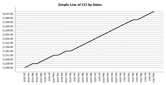
Figure 1.
Trend line of CCI from January 2019 to August 2021.
3.2. Descriptive Analysis and Pearson Correlation (I) of the Original Variables
Table 3 shows the descriptive statistics of the independent and the dependent variables. Table 4 shows the Pearson Correlation of the identified dependent and independent variables. The p-value (p) is the sig (2-tailed), which shows the correlation at both 95% and 99% confidence levels. The Building Permits, Consumer Price Index, Unemployment, Money Supply, Producer Price Index, Gross Domestic Products, and the Import Price Index demonstrate correlation to the construction cost index at 99% confidence level for the period under review with correction indexes of 0.726, 0.976, −0.706, 0.398, 0.853, 0.953, and 0.727 respectively. And the Crude Oil prices show a 95% confidence level of correlation to the CCI with a correlation index of 0.398. The employment rate for the period of January 2019 to August 2021 does not correlate with the construction cost index. The BP, CPI, MS, PPI, GDP, and IPI have a very strong positive relationship and the UNEMP has a very strong negative relationship, while the COIL has a weak positive relationship.
Table 3.
Selected descriptive statistics of identified variables from January 2019 to August 2021 (N = 32).
Table 4.
Pearson Correlation matrix for variables (N = 32).
3.3. Forecast of CCI Using Holt Model
A Holt model is adopted in forecasting the CCI from September 2021 to December 2022 to understand the changes in the CCI for the next 16 months and determine the fluctuations of the CCI, as well as the Upper and Lower Control Limits. The results (Table 5) are generated from the R Programming extension of the SPSS software (version 26.0, IBM, Armonk, NY, USA). A mean R-squared coefficient of 0.980 indicates 98% of the data values fit the regression model, showing a very strong fit for data analysis. This is a good indication because the dataset is very fit and can be used for further analysis. A lower (<0.50) co-efficient of model fit indicates that such results are weak and therefore would not be very useful for further analysis.
Table 5.
Model fit of the Construction Cost Index Forecast for the September 2021–December 2022.
A Mean Average Percentage Error of 0.217% indicates that the model prediction is excellent. MAPE < 10% is excellent and 20 < MAPE > 10 is good (Gilliland, 2010). Table 6 and Figure 2 below presents the forecast values of the CCI for September 2021 to December 2022. The results indicate the predicted values, the lower control limit (LCL), and the upper control limit (UCL) for the study period. It is worth noting that the CCI increases throughout the period under review. The UCL and LCL are critical indicators to determine whether variation in the process is stable and caused by an anticipated source. In this case, the CCI forecast line in Figure 2 is between UCL and LCL, so the observed variation in the forecast is due to random causes and probably occurs by chance. Additionally, this result indicates that the CCI forecast is stable.
Table 6.
Forecasted values of CCI for September 2021 to December 2022.

Figure 2.
Forecast of CCI for September 2021 to December 2022.
3.4. Forecast of Independent Variables for September 2021 to December 2022
The independent variables are forecasted for the period under review to understand the trends of changes that will occur for the next 16 months using the Autoregressive Integrated Moving Average (ARIMA) Model, the Winter’s Additive model, and the Simple Seasonal Model. Table 7 shows how these models are used for each analysis parameter in Section 2. Specifically, the analysis parameters are introduced in Table 1, and their data sources are listed in Table 2. The descriptive statistic values of these analysis parameters are in Table 3 and Table 4. The CCI predictions based on these parameters are in Table 5 and Table 6. After identifying the models for analysis parameters (a.k.a., independent variables) in Table 7, Table 8 shows the fitness analysis of the parameters. Notice that Table 7 and Table 8 are not for model comparison. Each coefficient in Table 8 is used to describe the quality of one model, isolated from other analyzes. When comparing different models, other statistics, such as the corrected R-squired (R2), centered R2, or information criteria of Likelihood Ration (LR) should be used. It is due to the different numbers of degrees of freedom (DF) of the analyzed models—resulting from a different number of estimated parameters. It can be seen even in the ARIMA models themselves. Therefore, the results in Table 8 are for the initial examination of the independent variables, not for model comparisons.
Table 7.
Models adopted for the Independent Variables.
Table 8.
Model fitness of the Independent Variables Forecast for the September 2021–December 2022.
The results in Table 8 indicate an overall R-squared coefficient of 0.847 depicting that 84.7% of all the independent variables fit the models adopted above. Hence, the forecasted values are a good fit for further analysis. However, Building Permit (BP) has an R-squared coefficient of 75.1%, Consumer Price Index (PPI) of 98.4%, Unemployment (UNEMP) of 73.6%, Employment (EMP) of 69%, Crude Oil (COIL) of 82.3%, Money Supply (MS) of 99.3%, Producer Price Index (PPI) of 97.4%, Gross Domestic Product (GDP) of 73.7%, and Import Price Index (IPI) of 93.4%. The Ljung-Box Q (18) test in Table 8 is for the absence of serial autocorrelation. Based on the Ljung Box Q (18) results, Model 4—shows no fit with a p-value of 0.042 (<5%), and model 1 with a p-value of 0.071 (<10%), it can be assumed that autocorrelation exists between these two models.
Table 9 shows that the results from the Simple Seasonal Model for the Unemployment (UNEMP) and Employment (EMP) parameters have the least R-squared coefficients of 73.6% and 69% respectively. The results from Winter’s Additive Model produce the fourth-least R-squared coefficient of 75.1%. The Autoregressive Integrated Moving Average (ARIMA) produces the highest R-squared coefficients which are CPI (98.4%), COIL (82.3%), MS (99.3%), PPI (97.4%), and IPI (93.4%). The overall Mean Absolute Percentage Error (MAPE) in Table 9 of all the independent variables is 5.519 indicating 5.52% of prediction error. It is less than 10%, showing that the model prediction is excellent. Thus MAPE < 10% is excellent and 20% > MAPE > 10% is good [37].
Table 9.
Model fit of the Independent Variables Forecast for the September 2021–December 2022.
Table 10 and Figure 3 show the predicted values for each of the independent variables and their respective months and years for prediction. Figure 4 illustrates the graphical presentation of the data presented in the table. The red line trend of Figure 4 shows the line trend of the existing or original data values of the independent variables from January 2019 to August 2021, and the blue line trend indicates the forecast for the next 16 months ending December 2022. It can be observed from the presentation that the Building Permits (BP), Consumer Price Index (CCI), the Money Supply (MS), and the Producer Price Index (PPI) have somewhat consistent trends from January 2019 to December 2022, while the rest of the variables have fluctuating trends.
Table 10.
Forecasted values September 2021 to December 2022.

Figure 3.
Forecast of Independent Variables for September 2021 to December 2022.

Figure 4.
Forecast of Transportation Metrix for September 2021 to December 2022.
3.5. Pearson Correlation (II) of Forecasted Independent and Dependent Variables
This study calculates a second Pearson Correlation of the forecasted values of the independent and dependent variables for the following purposes: (1) to understand what independent variables correlate with the CCI for the next 16 months starting September 2021 to December 2022 and (2) to verify the correlation generated from the original independent and dependent variables. The Holt forecasted model for the CCI generates a mean R-Squared coefficient of 98% and a MAPE of 0.217%, indicating that the prediction model is excellent and can be used for further analysis. The overall R-squared of the independent variables is 84.7% of model fit with a MAPE of 5.5% also indicates that the model is good for further analysis. Therefore, the results of the Pearson Correlation have high confidence of reliability.
The analysis shows that Building Permit, Consumer Price Index, Money Supply, Producer Price Index, and Import Price Index have a strong correlation with the Construction Cost Index at 99% confidence level. It is worth noting that Consumer Price Index, Money Supply, and Producer Price Index have a very strong positive correlation with the CCI, and Building Permit has a strong correlation. Meanwhile, the Import Price Index has a very strong negative correlation with the CCI at a 99% confidence level.
3.6. Impact of Transportation Metrics on the Construction Cost Index
This research establishes the Transportation Index from the Transportation Gross Domestic Product (GDP Transport), Transportation Consumer Price Index (CPI Transport), Transportation Service Index (TSI Freight). The first purpose is to analyze the correctness of predictions, and then secondly to check the model fit of the prediction from September 2021 to December 2022. Table 11 shows the Pearson Correlation of the variables. The CCI indicates that none of the variables have a correlation with the CCI neither at 95% nor 99% confidence levels.
Table 11.
Pearson Correction of CCI, CPI Transport, GDP Transport, and TSI Freight (N = 32).
3.7. Forecast of Transportation Metric
The purpose of this analysis is to determine a suitable model to forecast the Transportation Metrics, such as Transportation GDP, Transportation CPI, and Transportation Service Index (Freight). The data in Table 12 indicates that none of the proposed models (ARIMA and Simple Regression) is suitable to predict the metrics since the MAPE is very high with a low R-squared of 48% model fit as well.
Table 12.
Transportation metrics model fit.
In general, the data analysis focuses on the prediction aspect of construction costs and trends. The discussion on the predictive analytics process includes the increasing trend of CCI in 2022. The validation of the results uses descriptive analysis and Pearson correlations, which shows that building permits, consumer price index, money supply, producer price index, gross domestic products, and import price index have very strong positive relationships with the construction cost index. On the other hand, unemployment rates have a very strong negative relationship with the construction cost index. The results from the Holt model and the MAPE analysis also imply that the forecasts are highly reliable. Moreover, the analysis of the transportation metrics does not support the correlation between transportation development and construction costs.
The descriptive and predictive parameters and models demonstrate how they can be used in risk monitoring and control. Managers can use the discussion of CCI to develop risk prediction models and evaluate different risk control methods, such as penalized regression, ridge regression, and lasso regression when the construction industry is in a downtrend; or market development and penetration when the industry is in an uptrend. Managers should also be aware of the implementation limitations of the CCI forecasts, for example, the model overfitting issues of big data analytics and sample sizes.
4. Conclusions
Using the monthly CCI published by the ENR helps in budgeting for materials, labor, and other construction-related costs. One implication to practice is that other factors influence the CCI and should be taken into consideration. The analysis from our research shows that the number of building permits issued has a strong influence on the CCI. These results confirm the study by [13,16,18,38]. Also, the consumer price index, money supply, and producer price have a strong positive influence on the CCI, whilst the import price index has a very strong negative influence on the CCI, these results confirm the studies of [27]. In addition, the Autoregressive Integrated Moving Average (ARIMA) promises to be the most accurate prediction model with a minimum R-squared of 82.3% and maximum R-squared of 99.3%, the Winter Additive Simple Seasonal Model been the next accurate prediction model with an R-squared of 75%, and the Simple Season Model comes off with a minimum R-squared of 69% and a maximum R-squared of 73.6%. Construction managers and cost planners should adopt the ARIMA in their cost predictions as well as monitor the trends of building permits, consumer price index, money supply, producer price index, and import price index since they have a strong influence on the cost of materials, and labor.
According to the research results, it is important to provide adequate information about influencing factors and the corresponding risks with no ambiguity. This helps in developing a necessary response in risk monitoring and control, programming risk in cause-effect diagrams, and attributing ownership. The identified preliminary information, assumptions, background information, and the situation of the construction industry should be of substantial importance to project managers, senior managers, and directors of construction companies. The areas where uncertainties may occur should be identified and accurately described. In this way, the factors and their influences examined and discussed in this research will help construction companies to clearly understand and estimate the risks related to construction costs.
One limitation of this research is that machine learning techniques were not used for risk prediction. For example, future researchers could use machine learning and artificial neural networks to explore the relationships between transportation metrics, such as transportation gross domestic products, transportation consumer price index, transportation service index (freight), and CCI. This can help to determine whether changes in those indexes affect the costs of materials and labor in the construction industry.
Author Contributions
Conceptualization, H.X.; formal analysis, F.J., J.A. and H.X.; funding acquisition, F.J.; investigation, J.A. and H.X.; methodology, H.X.; project administration, F.J. and H.X.; resources, F.J. and H.X.; visualization, J.A.; writing—original draft, F.J., J.A. and H.X.; writing—review & editing, H.X. All authors have read and agreed to the published version of the manuscript.
Funding
This project is supported by the fund of Construction Project of Jiangsu Engineering Research Center “Jiangsu Province Engineering Research Center of Green Construction and BIM Technology Application for Complex Projects, (project number: JPERC2021-168)”.
Institutional Review Board Statement
Not applicable.
Informed Consent Statement
Not applicable.
Data Availability Statement
The data used for the analysis can be found through the links provided below.
- Construction Cost Index—https://www.enr.com/economics (accessed on 30 December 2021)
- Consumer Price Index—https://www.bls.gov/cpi/ (accessed on 30 December 2021)
- Unemployment Rate (general)—https://www.bls.gov/eag/eag.us.htm (accessed on 30 December 2021)
- Employment Rate (general)—https://www.bls.gov/ces/ (accessed on 30 December 2021)
- Producer Price Index—https://www.bls.gov/ppi/ (accessed on 30 December 2021)
- Crude Oil Prices—https://www.eia.gov/outlooks/steo/report/prices.php (accessed on 30 December 2021)
- Gross Domestic Product—https://www.bea.gov/data/gdp/gross-domestic-product (accessed on 30 December 2021)
- Building Permits—https://socds.huduser.gov/permits/ (accessed on 30 December 2021)
- US Import Price Index—https://www.bls.gov/mxp/ (accessed on 30 December 2021)
- Money supply—https://www.federalreserve.gov/releases/h6/current/default.htm (accessed on 30 December 2021)
Conflicts of Interest
The authors declare no conflict of interest.
References
- Leśniak, A.; Zima, K. Cost calculation of construction projects including sustainability factors using the Case Based Reasoning (CBR) method. Sustainability 2018, 10, 1608. [Google Scholar] [CrossRef] [Green Version]
- Alinizzi, M.; Haider, H.; Almoshaogeh, M.; Alharbi, F.; Alogla, S.M.; Al-Saadi, G.A. Sustainability Assessment of Construction Technologies for Large Pipelines on Urban Highways: Scenario Analysis using Fuzzy QFD. Sustainability 2020, 12, 2648. [Google Scholar] [CrossRef] [Green Version]
- Alvarenga, F.C. Analysis of the Causes of Food Additives Cost and Time in Public Works of Federal Educational Institutions. UFPA. Universidade Federal do Pará. 2019. Available online: http://repositorio.ufpa.br/jspui/bitstream/2011/11129/1/Dissertacao_Analisecausasaditivos.pdf (accessed on 30 December 2021).
- Plebankiewicz, E. Model of predicting cost overrun in construction projects. Sustainability 2018, 10, 4387. [Google Scholar] [CrossRef] [Green Version]
- Famiyeh, S.; Amoatey, C.T.; Adaku, E.; Agbenohevi, C.S. Major causes of construction time and cost overruns: A case of selected educational sector projects in Ghana. J. Eng. Des. Technol. 2017, 15, 181–198. [Google Scholar] [CrossRef]
- Elmousalami, H.H. Artificial intelligence and parametric construction cost estimate modeling: State-of-the-art review. J. Constr. Eng. Manag. 2020, 146, 03119008. [Google Scholar] [CrossRef]
- Zhang, R.; Ashuri, B.; Shyr, Y.; Deng, Y. Forecasting construction cost index based on visibility graph: A network approach. Phys. A Stat. Mech. Its Appl. 2018, 493, 239–252. [Google Scholar] [CrossRef]
- Cong, T.D.; Minh, Q.N. Estimating the construction schools cost in Ho Chi Minh City using Artificial Neural Network. In IOP Conference Series: Materials Science and Engineering; IOP Publishing: Bristol, UK, 2020; p. 062014. [Google Scholar]
- Mao, S.; Xiao, F. Time series forecasting based on complex network analysis. IEEE Access 2019, 7, 40220–40229. [Google Scholar] [CrossRef]
- Juan, Y.-K.; Liou, L.-E. Predicting the schedule and cost performance in public school building projects in Taiwan. J. Civ. Eng. Manag. 2021, 28, 51–67. [Google Scholar] [CrossRef]
- Assaad, R.; El-Adaway, I.H.; Abotaleb, I.S. Predicting project performance in the construction industry. J. Constr. Eng. Manag. 2020, 146, 04020030. [Google Scholar] [CrossRef]
- Elfahham, Y. Estimation and prediction of construction cost index using neural networks, time series, and regression. Alex. Eng. J. 2019, 58, 499–506. [Google Scholar] [CrossRef]
- Shahandashti, S.M.; Ashuri, B. Highway construction cost forecasting using vector error correction models. J. Manag. Eng. 2016, 32, 04015040. [Google Scholar] [CrossRef]
- Ghodoosi, F.; Abu-Samra, S.; Zeynalian, M.; Zayed, T. Maintenance cost optimization for bridge structures using system reliability analysis and genetic algorithms. J. Constr. Eng. Manag. 2018, 144, 04017116. [Google Scholar] [CrossRef]
- Hassim, S.; Muniandy, R.; Alias, A.H.; Abdullah, P. Construction tender price estimation standardization (TPES) in Malaysia: Modeling using fuzzy neural network. Eng. Constr. Archit. Manag. 2018, 25, 443–457. [Google Scholar] [CrossRef]
- Ashuri, B.; Lu, J. Time series analysis of ENR construction cost index. J. Constr. Eng. Manag. 2010, 136, 1227–1237. [Google Scholar] [CrossRef]
- Wang, J.; Ashuri, B. Predicting ENR construction cost index using machine-learning algorithms. Int. J. Constr. Educ. Res. 2017, 13, 47–63. [Google Scholar] [CrossRef]
- Shahandashti, S.M.; Ashuri, B. Forecasting engineering news-record construction cost index using multivariate time series models. J. Constr. Eng. Manag. 2013, 139, 1237–1243. [Google Scholar] [CrossRef]
- Juszczyk, M.; Leśniak, A. Modelling construction site cost index based on neural network ensembles. Symmetry 2019, 11, 411. [Google Scholar] [CrossRef] [Green Version]
- Tarmizi, H.; Daulay, M.; Muda, I. Impact of the economic growth and acquisition of land to the construction cost index in North Sumatra. In IOP Conference Series: Materials Science and Engineering; IOP Publishing: Bristol, UK, 2017; p. 012004. [Google Scholar]
- Moon, S.; Chi, S.; Kim, D.Y. Predicting Construction Cost Index Using the Autoregressive Fractionally Integrated Moving Average Model. J. Manag. Eng. 2017, 34, 04017063. [Google Scholar] [CrossRef]
- Caffieri, J.J.; Love, P.E.; Whyte, A.; Ahiaga-Dagbui, D.D. Planning for production in construction: Controlling costs in major capital projects. Prod. Plan. Control 2018, 29, 41–50. [Google Scholar] [CrossRef]
- Ilbeigi, M.; Ashuri, B.; Joukar, A. Time-series analysis for forecasting asphalt-cement price. J. Manag. Eng. 2017, 33, 04016030. [Google Scholar] [CrossRef]
- Ilbeigi, M.; Castro-Lacouture, D.; Joukar, A. Generalized autoregressive conditional heteroscedasticity model to quantify and forecast uncertainty in the price of asphalt cement. J. Manag. Eng. 2017, 33, 04017026. [Google Scholar] [CrossRef]
- Joukar, A.; Nahmens, I. Volatility forecast of construction cost index using general autoregressive conditional heteroskedastic method. J. Constr. Eng. Manag. 2015, 142, 04015051. [Google Scholar] [CrossRef]
- Tajani, F.; Morano, P.; Saez-Perez, M.P.; Di Liddo, F.; Locurcio, M. Multivariate dynamic analysis and forecasting models of future property bubbles: Empirical applications to the housing markets of Spanish metropolitan cities. Sustainability 2019, 11, 3575. [Google Scholar] [CrossRef] [Green Version]
- Hellaoui, H.; Bekkouche, O.; Bagaa, M.; Taleb, T. Aerial control system for spectrum efficiency in UAV-to-cellular communications. IEEE Commun. Mag. 2018, 56, 108–113. [Google Scholar] [CrossRef]
- Chimdi, J.; Girma, S.; Mosisa, A.; Mitiku, D. Assessment of factors affecting accuracy of cost estimation in public building construction projects in western oromia region, Ethiopia. J. Civ. Eng. Sci. Technol. 2020, 11, 111–124. [Google Scholar] [CrossRef]
- Ibrahim, A.H.; Elshwadfy, L.M. Assessment of Construction Project Cost Estimating Accuracy in Egypt. Open Civ. Eng. J. 2021, 15, 290–298. [Google Scholar] [CrossRef]
- ENR. Construction Cost Index (CCI). 2021. Available online: https://www.enr.com/economics (accessed on 20 January 2022).
- BLS. U.S. Bureau of Labor Statistics. 2021. Available online: https://www.bls.gov/ (accessed on 20 January 2022).
- EIA. U.S. Energy Information Administration. 2021. Available online: https://www.eia.gov/ (accessed on 20 January 2022).
- BEA. U.S. Bureau of Economic Analysis. 2021. Available online: https://www.bea.gov/ (accessed on 20 January 2022).
- Census. U.S. Census Bureau. 2021. Available online: https://data.census.gov/cedsci/ (accessed on 20 January 2022).
- HUD. Department of Housing and Urban Development. 2021. Available online: https://www.huduser.gov/portal/pdrdatas_landing.html (accessed on 20 January 2022).
- Reserve. U.S. Board of Governors of the Federal Reserve System. 2021. Available online: https://www.federalreserve.gov/ (accessed on 20 January 2022).
- Gilliland, M. FVA: A Reality Check on Forecasting Practices. Int. J. Appl. Forecast. 2013. Available online: https://forecasters.org/wp-content/uploads/FVA_A-Reality-Check_Foresight29.pdf (accessed on 30 December 2021).
- Jallan, Y.; Brogan, E.; Ashuri, B.; Clevenger, C.M. Application of Natural Language Processing and Text Mining to Identify Patterns in Construction-Defect Litigation Cases. J. Leg. Aff. Disput. Resolut. Eng. Constr. 2019, 11, 04519024. [Google Scholar] [CrossRef]
Publisher’s Note: MDPI stays neutral with regard to jurisdictional claims in published maps and institutional affiliations. |
© 2022 by the authors. Licensee MDPI, Basel, Switzerland. This article is an open access article distributed under the terms and conditions of the Creative Commons Attribution (CC BY) license (https://creativecommons.org/licenses/by/4.0/).