Abstract
In this work, an enhanced slime mould algorithm (ESMA) based on neighborhood dimension learning (NDL) search strategy is proposed for solving the optimal power flow (OPF) problem. Before using the proposed ESMA for solving the OPF problem, its validity is verified by an experiment using 23 benchmark functions and compared with the original SMA, and three other recent optimization algorithms. Consequently, the ESMA is used to solve a modified power flow model including both conventional energy, represented by thermal power generators (TPGs), and renewable energy represented by wind power generators (WPGs) and solar photovoltaic generators (SPGs). Despite the important role of WPGs and SPGs in reducing CO2 emissions, they represent a big challenge for the OPF problem due to their intermittent output powers. To forecast the intermittent output powers from SPGs and WPGs, Lognormal and Weibull probability density functions (PDFs) are used, respectively. The objective function of the OPF has two extra costs, penalty cost and reserve cost. The penalty cost is added to formulate the underestimation of the produced power from the WPGs and SPGs, while the reserve cost is added to formulate the case of overestimation. Moreover, to decrease CO2 emissions from TPGs, a direct carbon tax is added to the objective function in some cases. The uncertainty of load demand represents also another challenge for the OPF that must be taken into consideration while solving it. In this study, the uncertainty of load demand is represented by the normal PDF. Simulation results of ESMA for solving the OPF are compared with the results of the conventional SMA and two further optimization methods. The simulation results obtained in this research show that ESMA is more effective in finding the optimal solution of the OPF problem with regard to minimizing the total power cost and the convergence of solution.
1. Introduction
Optimal power flow (OPF) has been a crucial tool for power systems’ operation in an efficient and secured way since its inception in 1962 by Carpentier [1]. OPF is employed for many objectives in power system such as minimizing total generation cost, reducing CO2 emissions, minimizing power losses, and maintaining voltage stability, as well as maintaining the optimal settings of control variables. This process is commonly constrained by set of restrictions which have to be satisfied, such as power generator capability, bus voltage, transmission line capacity, and any other technical constraints. Conventional OPF problem deals with fossil fuels power stations. When the penetration level of solar photovoltaic (PV) and wind power into the grid increases, it is necessary to study OPF problem taking into consideration the uncertain nature of these sources. In addition to the uncertainty in generation side, there is also uncertainty in the load side that can occur due to several factors such as the induction of electric vehicles [2,3]. Without taking this uncertainty into our consideration, realized load values will differ from the forecast values of load demand, and consequently, the planned operational state through the OPF might be non-optimal.
In the literature, different methods have been provided to model renewable energy sources (RESs) and load demand uncertainties. G-best guided artificial bee colony is provided in [4] to enhance OPF results that are verified in the past literature with similar experimental conditions. In [5], the authors proposed a modified bacteria foraging algorithm to find the best solution of OPF problem that incorporates with a mixture model for thermal power, wind power, and static synchronous compensator (STATCOM). In [6], the authors studied the OPF problem with and without wind power using the particle swarm optimization algorithm, and the Weibull distribution function was used to model the uncertain wind power generation. Reference [7] provided an OPF problem with comprehensive modeling of uncertainty in solar and wind power depending on a combination between success history-based adaptation of differential evolution and the superiority of feasible solution (SF) that is a methodology for handling constraints. The authors in [8] provided a full review of the OPF problem in its diverse formulas. OPF with traditional sources, RESs, and energy storage systems was studied. In [9], a genetic algorithm, the two-point estimation method, and Monte Carlo simulation were applied to solve the OPF problem including RESs and an energy storage system, and the uncertain nature of wind, solar, and load demand was handled by a new strategy. In [10], the authors presented a novel heap optimization algorithm (HOA) to find the optimal solution of the power flow. HOA-based OPF methodology is flexible and applicable compared with that achieved by using the genetic algorithm. A security constrained OPF (SCOPF) problem was studied in [11] incorporating wind energy and responsive demands. Gaussian distribution and Beta distribution were chosen for modeling the load demand and wind power, respectively. The authors assume operating costs, emission, and security indices as single and multi-objective functions. In [12], the OPF problem was studied incorporating several flexible AC transmission system (FACTS) devices with uncertain wind power and uncertain load demand. The uncertain output power of RESs and load demand are handled in [13] by providing uncertainty probability distribution to optimize the conventional generation. In [14], the authors developed an OPF model with stochastic wind power depending on the Lévy coyote optimization algorithm.
The Slime mould algorithm (SMA) is used in many research studies to solve the OPF problem and the economic dispatch. Like many metaheuristic optimization algorithms, SMA suffers from premature convergence during solving complex nonlinear problems. It also suffers from the insufficient precision of optimization and slow optimization speed, which may lead to easily falling into a local optima [15,16,17,18].
In this paper, an enhanced slime mould algorithm (ESMA) is proposed to overcome the drawbacks of the original SMA for solving the OPF problem. The ESMA is proposed by modifying the original SMA based on the neighborhood dimension learning (NDL) search strategy. The validity of the ESMA was tested experimentally through 23 benchmark functions. It was compared with the original (SMA) [19] and three other recent optimization algorithms, including the colony predation algorithm (CPA) [20], the aquila optimizer (AO) [21], and Runge Kutta (RUN) algorithm [22]. A modified IEEE 30–bus system incorporating one SPG and two WPGs was used for testing the validity of the proposed algorithm in reaching the optimal solution for OPF problem with uncertain renewable energy sources (RESs), variable load demand and ramp rate effect of TPGs, in addition to some theoretical cases. Two other optimization algorithms: black widow optimization algorithm (BWOA) [23], and moth swarm algorithm (MSA) [24], in addition to SMA [19] were applied for solving the OPF problem with the same conditions to verify the validity of ESMA comparing to other algorithms. The remaining sections of this research are organized as follows: Section 2 presents the mathematical modeling and the associated system constraints that are applied on the objective functions of the OPF problem. Then, Section 3 provides the modeling of the uncertain output of WPG and SPG. Section 4 presents the ESMA to solve the OPF problem incorporating the uncertain RESs. In Section 5, simulation results are provided including several practical case studies with the four applied algorithms. Finally, conclusions of this paper are presented in Section 6.
2. Problem Formulation
TPGs have constant power outputs, while WPGs and SPG have variable power outputs that must be balanced with the aid of the energy mix of all involved generators and the reserve power, thus the total power cost consists of the operation costs for all the involved power generators, penalty cost, and reserve cost. In this subsection, the cost models of all power generators involved in the objective function of the OPF is performed as follows.
2.1. Cost Model of TPGs
Fossil fuel is used to operate TPGs. Equation (1) shows how to calculate the fossil fuel cost ($/h) of all TPGs.
The valve-point loading has an impact on the total fuel cost, so taking it into consideration will give more realistic and precise cost as shown in (2).
All coefficients of cost and emission for the TPGs that are used in cost calculations are recorded in Table 1.

Table 1.
Cost and emission Coefficients for TPGs [25].
2.2. Direct Power Cost of SPG and WPGs
When private parties have the ownership of SPG or WPG, independent system operators (ISO) will pay an amount of money proportional to the contractually scheduled output powers.
In this concept, the direct cost of wind power produced from the jth WPG in proportion to its scheduled power has been provided in (3).
Following the same method, the direct cost of the kth SPG can be modelled by
2.3. Cost Assessment for Uncertain Wind Power Output
One of the most challenging characteristics of wind energy is its intermittent output, so two situations might arise. The first one happens if the actual output power from the WPG is lower than the anticipated power output. This means that there is an overestimation of the output of WPGs. In this case, ISO uses the spinning power reserved for maintaining the reliability of the supplied power to its consumers.
To overcome this situation, reserve cost is need to committee reserve power units. This cost can be determined for the jth WPG as follows:
The other situation happens if the actual output of the WPG has a value greater than expected. This means that there is an underestimation in the output power. Then, there will be a remaining power that will be dissipated if there is not any possibility to decrease the output of TPGs. In this regard, ISO should pay a penalty cost according to the rest power. This cost can be determined for the jth WPG by
2.4. Cost Assessment for Uncertain Solar PV Power
Solar output power has also intermittent and uncertain nature, so the same concept followed to deal with underestimation and overestimation scenarios of output power of WPGs will be followed with solar energy. In this work, solar radiation will follow lognormal probability density functions (PDF) [26], which differs from the Weibull PDF followed by wind power.
Thus, for making calculations simpler, the models of penalty cost and reserve cost are designed in a similar concept used in [27].
Section 3 provides more details for stochastic wind and solar power calculation.
For the kth SPG, the reserve cost is given as follows:
Equation (8) shows the formulation of the penalty cost corresponding to the kth SPG.
2.5. Emissions and Carbon Tax
Producing electricity through burning fossil fuels is one of the most emitting sources of greenhouse gases into the surrounding environment. Emissions are determined in (t/h) as follows:
The emission coefficients values of the TPGs provided in Table 1 are the same as in [25] with only small modification in the value of μ of the TPG connected at bus 1.
Due to the dangerous effects associated with climate change phenomena, regulators in many countries tend to set severe rules on power sectors to diminish the carbon emission (carbon footprint) [28] by applying a carbon tax which is one of the most useful methods for pushing investors towards renewable energy projects. The emission cost ($/h) is determined by
2.6. Objective Functions of the OPF
The objective function (F1) of the OPF include all the previously presented cost models from (2) to (8). F1 neglects the cost of emissions, while another objective function (F2) is proposed with considering the cost of emissions to study its impact on the generation scheduling. F2 is expressed with the same cost models used in F1 in addition to the cost of emissions provided in (9) and (10).
Hence, the objective is to minimize F1 shown in (11):
To minimize F2 that is formulated as follows:
Both system equality and inequality constraints are imposed on the above mentioned OPF objective functions as shown below:
2.6.1. Equality Constraints
To provide an active and reactive power balance in the system, equality constraints should be applied for the system. Equality means that these active and reactive powers should be equivalent to summation of total load and total power loss in the network. Consequently, equality constraints have been given as follows [7]:
2.6.2. Inequality Constraints
Equipment and components existing in any power system operate within operating limits which are called inequality constraints. These constraints can be expressed as follows:
- 1.
- Constraints of Generators:
Equations (15)–(17) represent the limits of active power generation for TPGs, WPGs, and SPGs, respectively.
Reactive power limits of all generators are showed by (18) to (20) with the same arrangement in the previous active power limits equations.
Equation (21) shows the constraints applied on generator buses voltage.
- 2.
- Security constraints:
The voltage limits applied to load buses are shown by (22), while (23) gives the capacity constraints of transmission lines.
The active power losses (Ploss) in transmission lines and voltage deviation (Vd) represent also essential parameters when studying OPF problem. It is not allowable to avoid the active power loss in transmission lines because of their inherent resistances. Ploss of the grid is given by
Equation (25) refers to the voltage deviation (Vd) which indicates how much load buses voltages, in a power system, deviate from a nominal voltage value which usually is 1 p.u. Vd gives a sign for the voltage quality of the power system.
- 3.
- TPGs Ramp Rate Constraints:
In practical conditions, the produced power from a thermal power generator should follow ramp rates because of the physical limitations of thermal generators. This means that to rise the generated power from a thermal generator, it follows the up-ramp rate. In contrast, to reduce the generated power, it follows the down-ramp rate. In this regard, the limits of ramp rate can be formed as follows:
The constraints of ramp-rate in OPF study are formulated as following:
It is worth pointing out that the presence of ramp-rate limits will increase the cost of generation due to changing the new operating points of TPGs from their original operating points without ramp rate constraints. The new limits of a TPG with limits of ramp-rate should not outdo the limits () and () which are provided in (27) and (28), respectively.
3. Stochastic Solar Power, Wind Power, and Models of Uncertainty
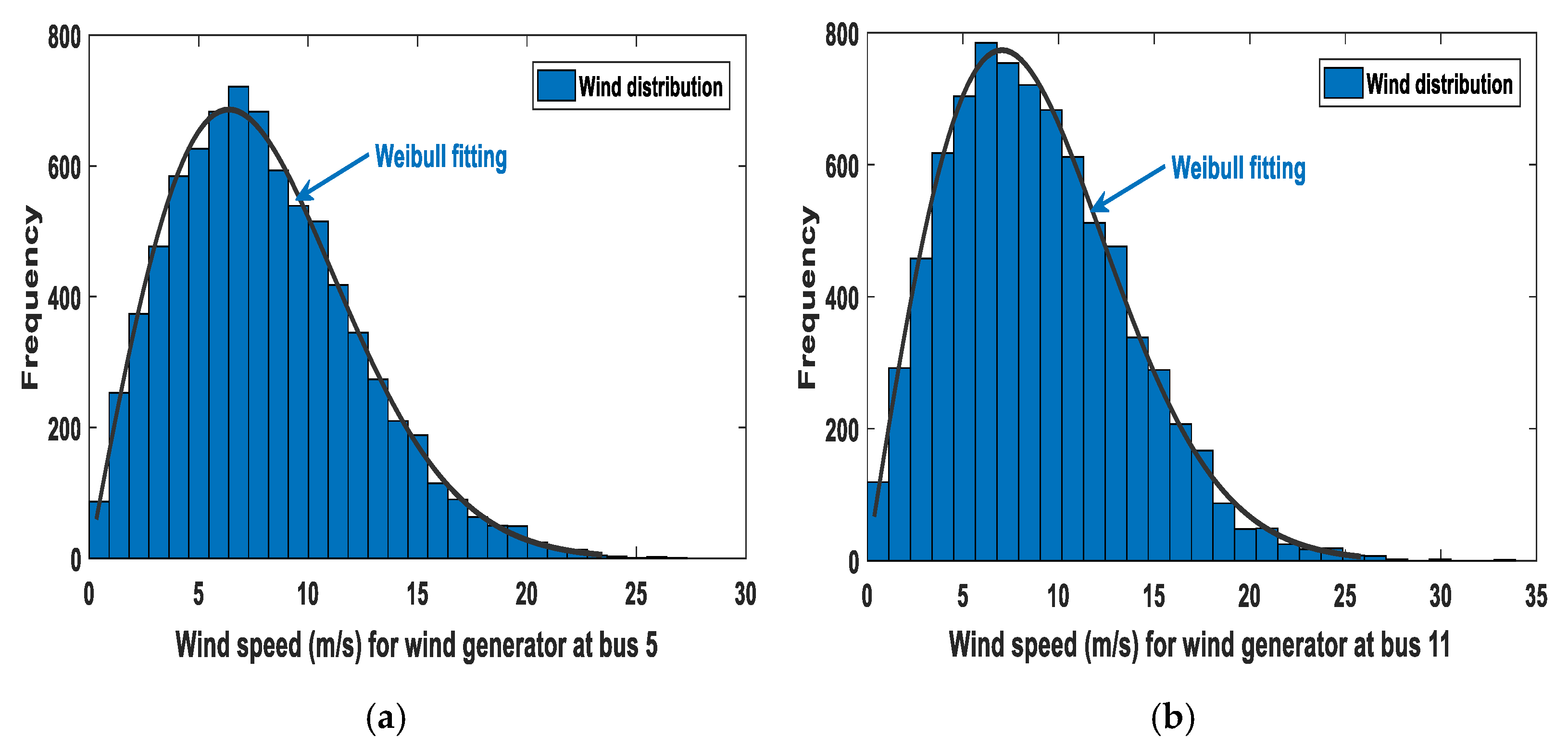
This Weibull PDF is followed by wind speed distribution for calculations of mean power of wind turbines as presented in [5,27]. The probability () of wind speed () in (m/s) based on Weibull PDF has been provided as follows:
In (30), the mean of Weibull PDF is defined as follows:
where, indicates gamma function which is defined as
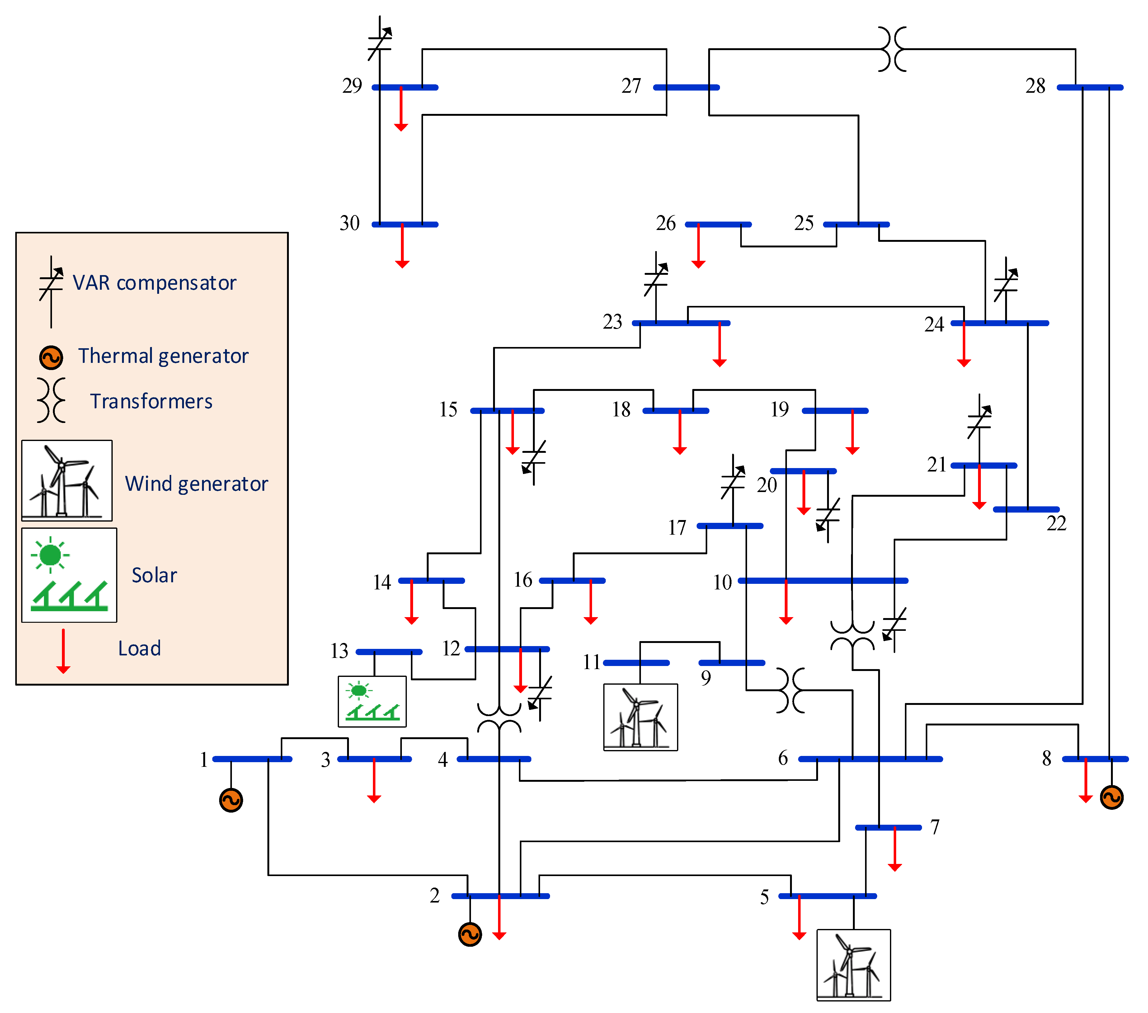
In this study, the IEEE-30 bus system is modified via replacing two TPGs at bus 5 and bus 11 with two WPGs in addition to replacing TPG at bus 13 with SPG, as shown in Figure 1. Other system characteristics are provided in Table 2. The selected values of Weibull scale () and shape () parameters are mentioned in Table 3. Weibull fitting and distributions of wind frequency are provided in Figure 2. They are obtained through Monte Carlo simulation running with 8000 iterations [7].
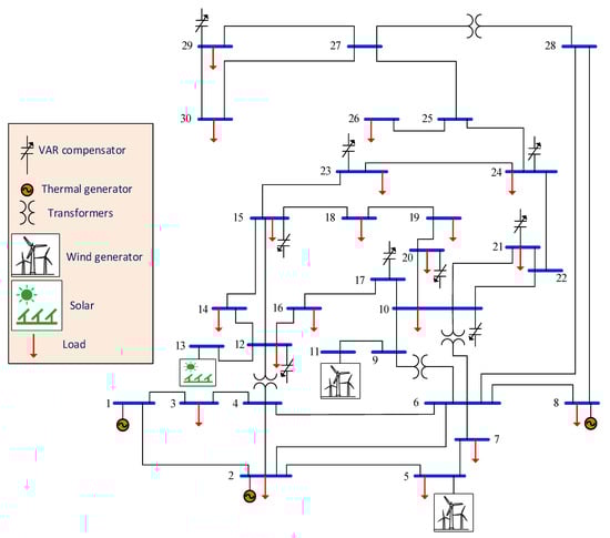
Figure 1.
Modified IEEE-30 bus power system.
Table 2.
Characteristics of the modified IEEE-30 bus system [7].
Table 3.
Weibull and lognormal PDF Parameters for WPGs and SPG.

Figure 2.
Wind speed distribution for WPGs, (a) WPG1 at bus 5 (c = 9, k = 2) and (b) WPG2 at bus 11 (c = 10, k = 2).
Standard [30] regulates the design requirements of wind turbines and determines wind turbine class IA which is the highest turbulent and proper for operating at the maximum annual average wind speed of 10 m/s at hub height. Parameters of wind farm scale () and shape (), have been chosen sensibly in order to keep the mean of Weibull PDF at a maximum value nearby 10. This will help in reaching both diverse and realistic geographic places for the two WPGs.
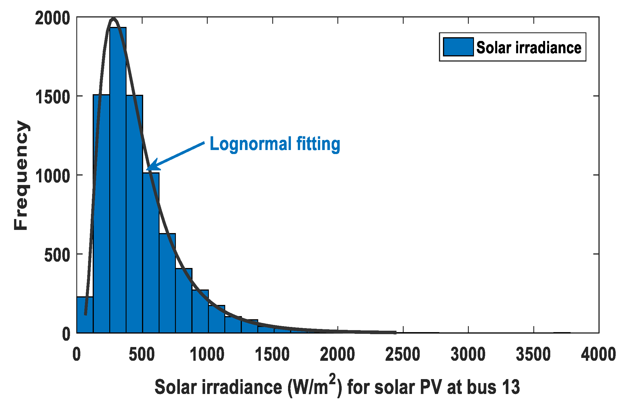
The output power from the SPG is in a direct relationship with the irradiance (I) that tracks lognormal PDF [26]. The solar irradiance probability with standard deviation () and mean (), is determined by
Equation (33) presents the mean parameter of the lognormal PDF ().
The distribution of frequency and lognormal probability for the solar irradiance obtained by running Monte-Carlo simulation with a sample size of 8000 iterations are shown in Figure 3. The selected values of lognormal PDF parameters are provided in Table 3.
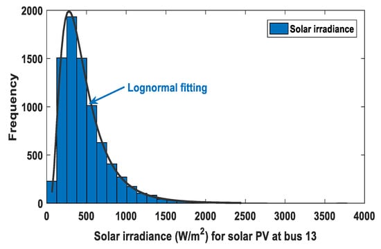
Figure 3.
Solar irradiance distribution for SPG ( μ = 6).
3.1. Models of Solar and Wind Powers
As previously demonstrated, there are two WPGs in the new IEEE-30 bus power system. WPG 1 is linked to bus 5, and its cumulative active power is 75 MW. WPG 2 is linked to bus 11, and its cumulative active power equals 60 MW.
The output power of a wind turbine () depends on the speed of wind () as described below [7]:
Enercon E82-E4, which is a product datasheet of wind turbine, states the different speeds of a wind turbine with rated power 3 MW as follows: = 3 m/s, = 25 m/s, and = 16 m/s.
Likewise, the output power of SPG, depending on solar irradiance (I), as stated below [31]:
3.2. Probability Calculation of Wind Power
The output power of WPG, according to (34), has a discrete nature in certain wind speed regions. The value of power output will be zero when the value of is below and above , while the wind turbine will produce the rated value when the value of is between and . For the illustrated discrete zones, the probabilities of wind turbine output power are provided by [32]:
The wind turbine has a continuous output power between and . Thus, for the continuous zone, the probabilities of wind turbine output power are provided by [33]
3.3. Over/Underestimation Cost of Solar Power
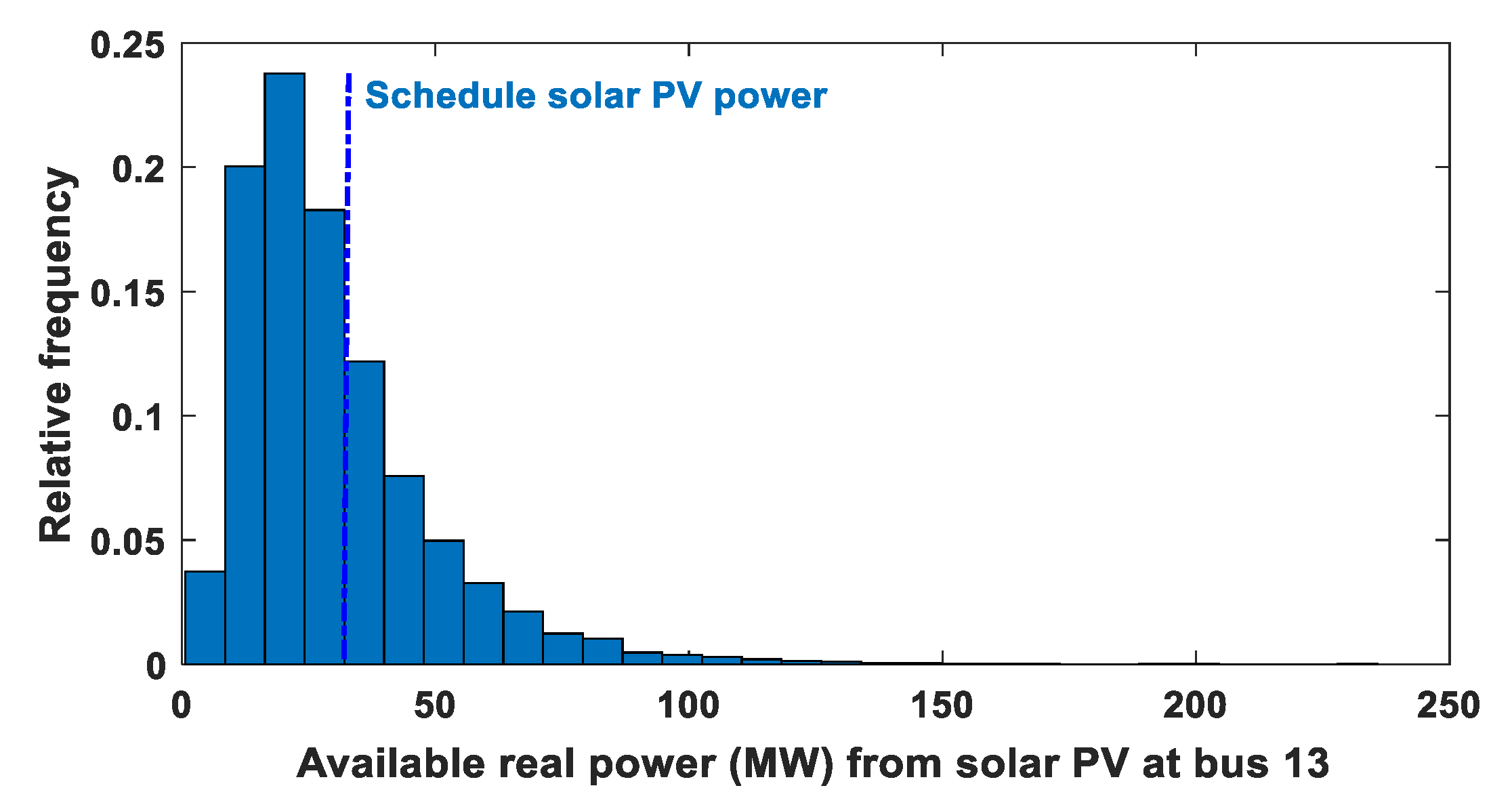
The SPG produces a power that has a stochastic nature. Figure 4 verifies this nature, and it also defines the scheduled output power of the SPG to be transferred to the grid through the dotted line. It is important to notice that the scheduled power of SPG is an inconstant value, thus the owner of the SPG and the ISO should sign a jointly power agreement. Equations (39) and (40) are developed for calculating the cost of under- and overestimation () in the output power of the SPG, respectively.
where and indicate the surplus and shortage powers which lie on the left and right half plane of schedule power in Figure 4, respectively. Similarly, represent relative frequencies of the happening of . While are the numbers of discrete bins lie on the right and left plane of for the generation of PDF, respectively.

Figure 4.
Real power (MW) distribution for SPG at bus 13.
4. Optimization Algorithm
4.1. Original SMA
The slime mould optimization algorithm is developed in [19]. It generally denotes the physarum polycephalum and it has been named by this name because its first classification was under category of fungus [34].
The mathematical model of SMA is as follows [19]:
4.1.1. Food Approach
Based on the smell in the surrounding air, slime mould can approach food [19]. Equations (41)–(44) is provided to imitate the contraction method:
The slime mould weight () is calculated as follows:
In (45), condition means that S(i) ranks the first half of population.
4.1.2. Wrap Food
The mathematical approach followed by slime mould for updating its location is as follows:
4.1.3. Grabble Food
This mathematical approach means that if the concentration of food is high, the weight close to the region is bigger. On the other hand, if the concentration of food is little, the weight close to the region will decrease and hence it decides to turn to explore other areas.
represents a vector that has random values oscillates in the range of [−a, a] and gradually accesses zero with the iterations increment. Values of have been taken in the range of [−1, 1] and eventually tend towards zero. Synergistic interaction that takes place between and provides a simulation for the selective behavior of slime mould. It will keep distributing organic material for exploring other regions, even if it found a better food source, trying to find a food source with higher quality instead of using all of it in one source.
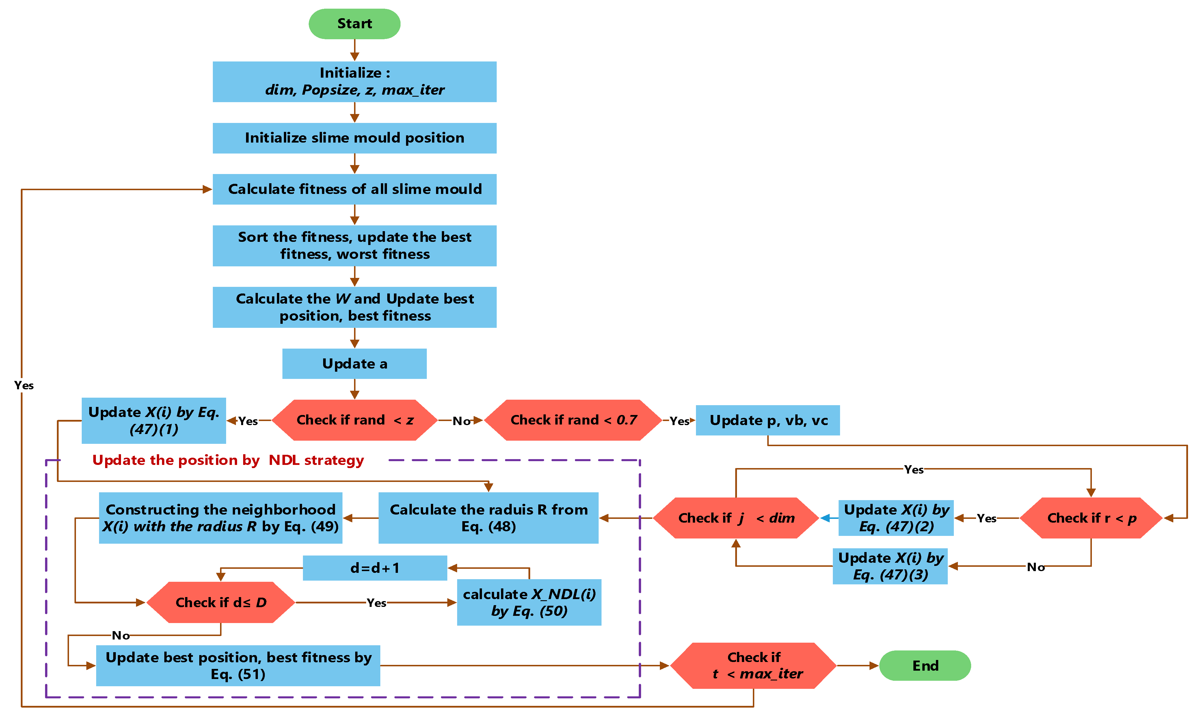
4.2. Proposed ESMA
The ESMA is developed by the neighborhood dimension learning (NDL) search strategy to improve the search abilities of the ESMA and to make the exploration-exploitation more balanced [35]. In this strategy, firstly, a radius () is defined by Euclidean distance () between the current location of and the candidate location from the following equation:
Then, the neighbors of denoted by is formed by (49) considered to :
As soon as the neighborhood of is formed, multi neighbors learning are performed using this equation:
where d-th dimension of is computed by the d-th dimension of a random of neighbor chosen from , and a random position from the population of slime mould.
Finally, selecting the best position is given using (51).
The flow chart of ESMA is shown in Figure 5.
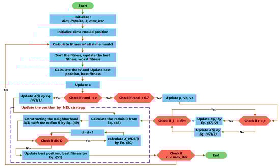
Figure 5.
ESMA flow chart.
5. Results
5.1. Performance of the Proposed ESMA Algorithm
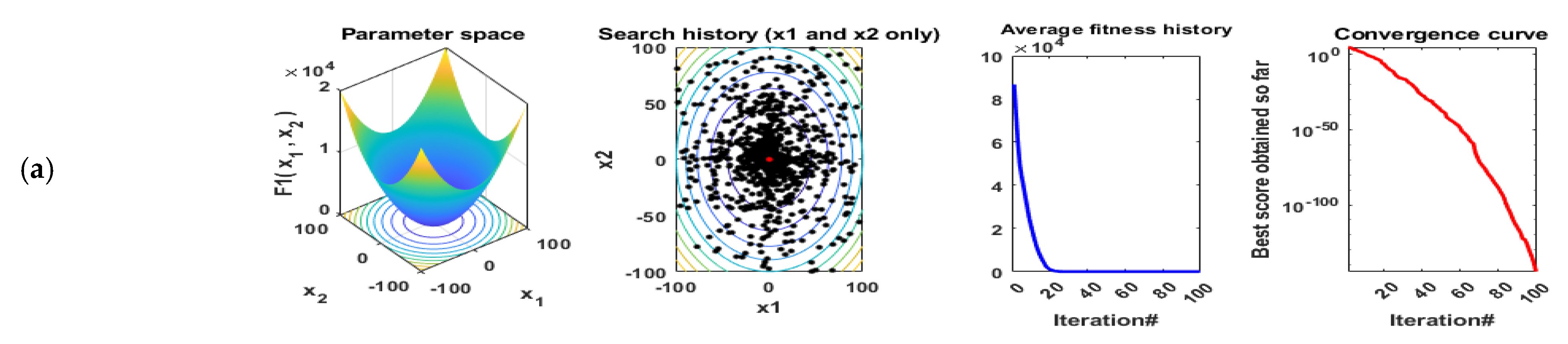
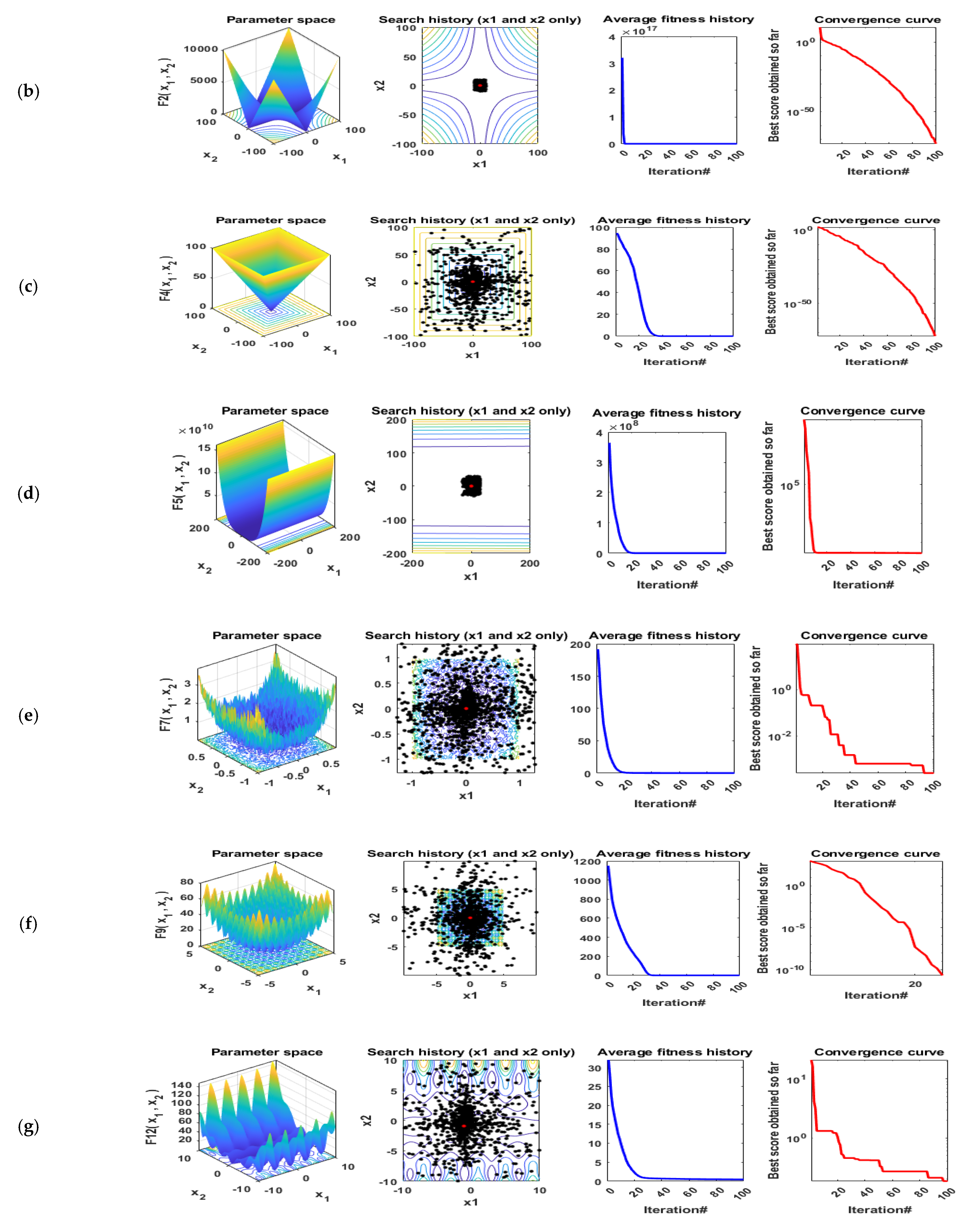
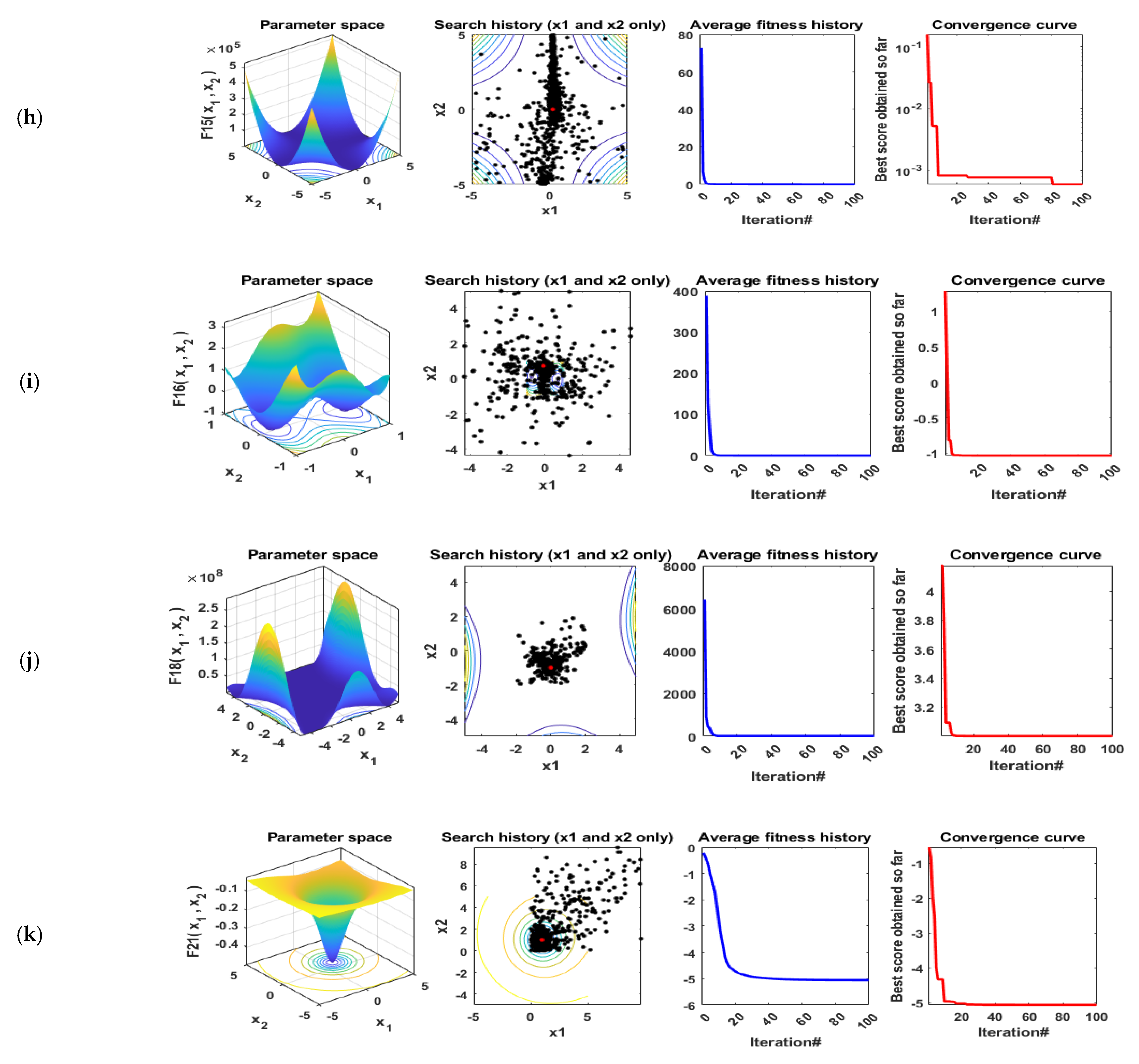
In this subsection, the effectiveness and performance of the proposed ESMA algorithm are evaluated on many benchmark functions including the best values, mean values, worst values, and standard deviation (STD) for the solutions obtained by the ESMA technique, the original SMA algorithm, and the three recent optimization algorithms, including CPA, AO, and RUN. The results of the proposed ESMA algorithm are compared with these well known optimization algorithms. These algorithms have been performed in 20 independent runs. The maximum number of iterations for each run is 200 and the population size is 50. All simulations were executed using MATLAB R2016a on a laptop including Core i5-4210U CPU@2.40 GHz of speed, and 8 GB of RAM. Figure 6 illustrates the qualitative metrics using ESMA algorithm for 11 benchmark functions including 2D views of the functions, search history, average fitness history, and convergence curve.
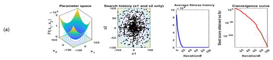
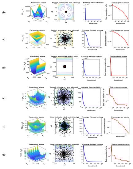
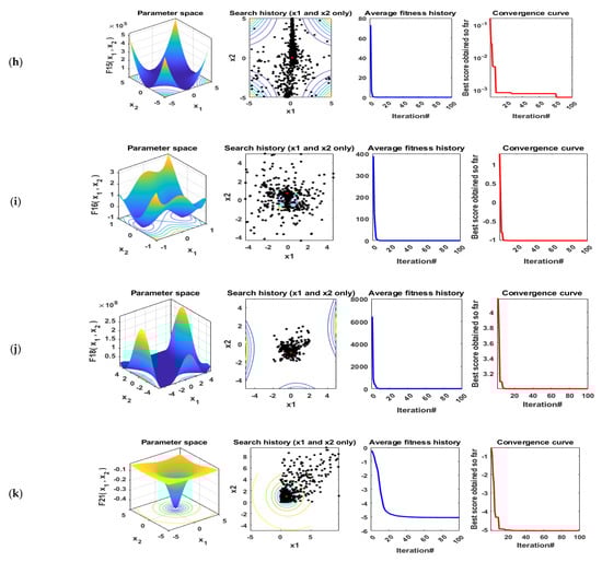
Figure 6.
Qualitative metrics of 11 benchmark functions: 2D views of the functions, search history, average fitness history, and convergence curve using ESMA algorithm. (a) F1; (b) F2; (c) F4; (d) F5; (e) F7; (f) F9; (g) F12; (h) F15; (i) F16; (j) F18; (k) F21.
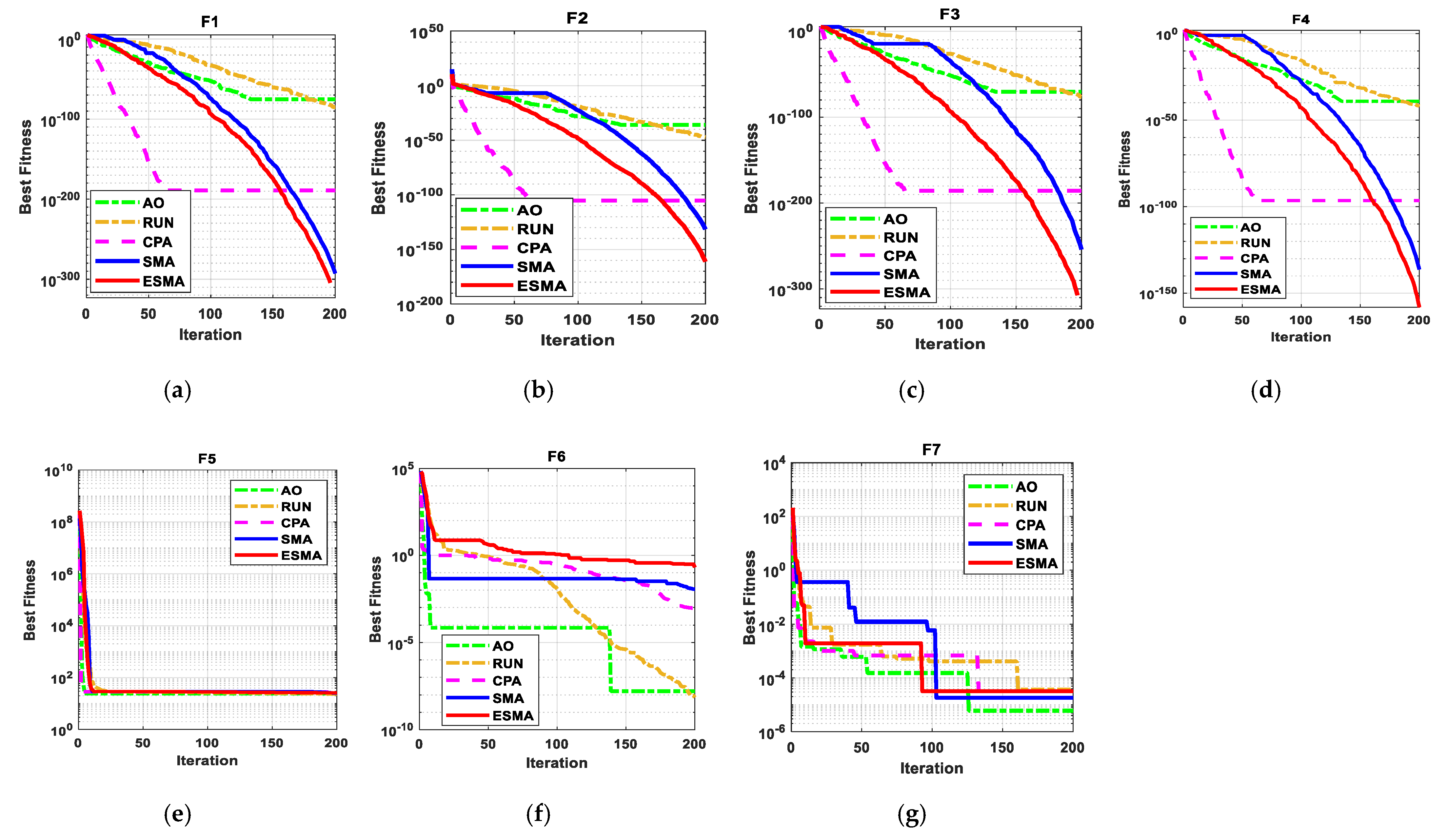
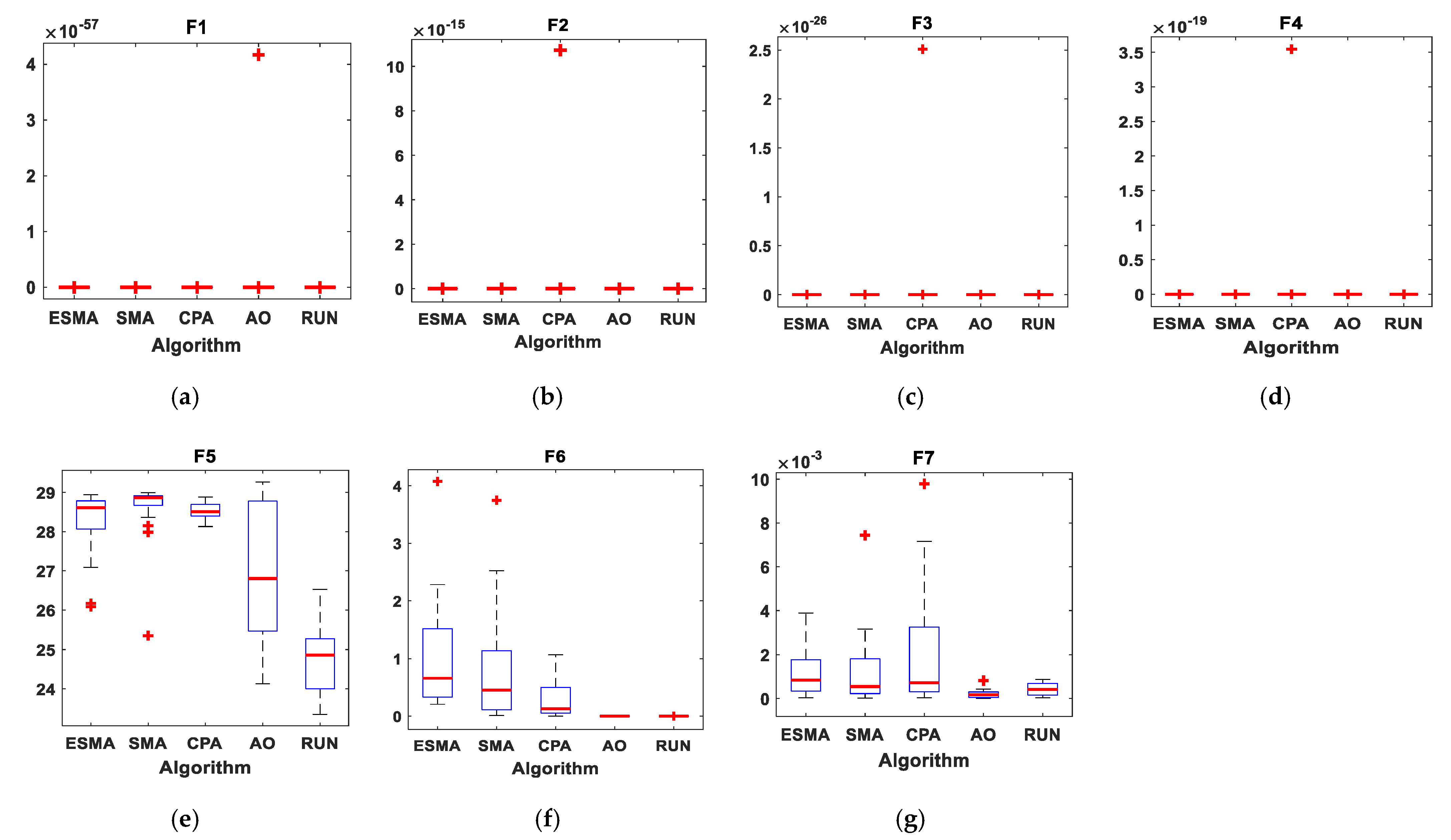
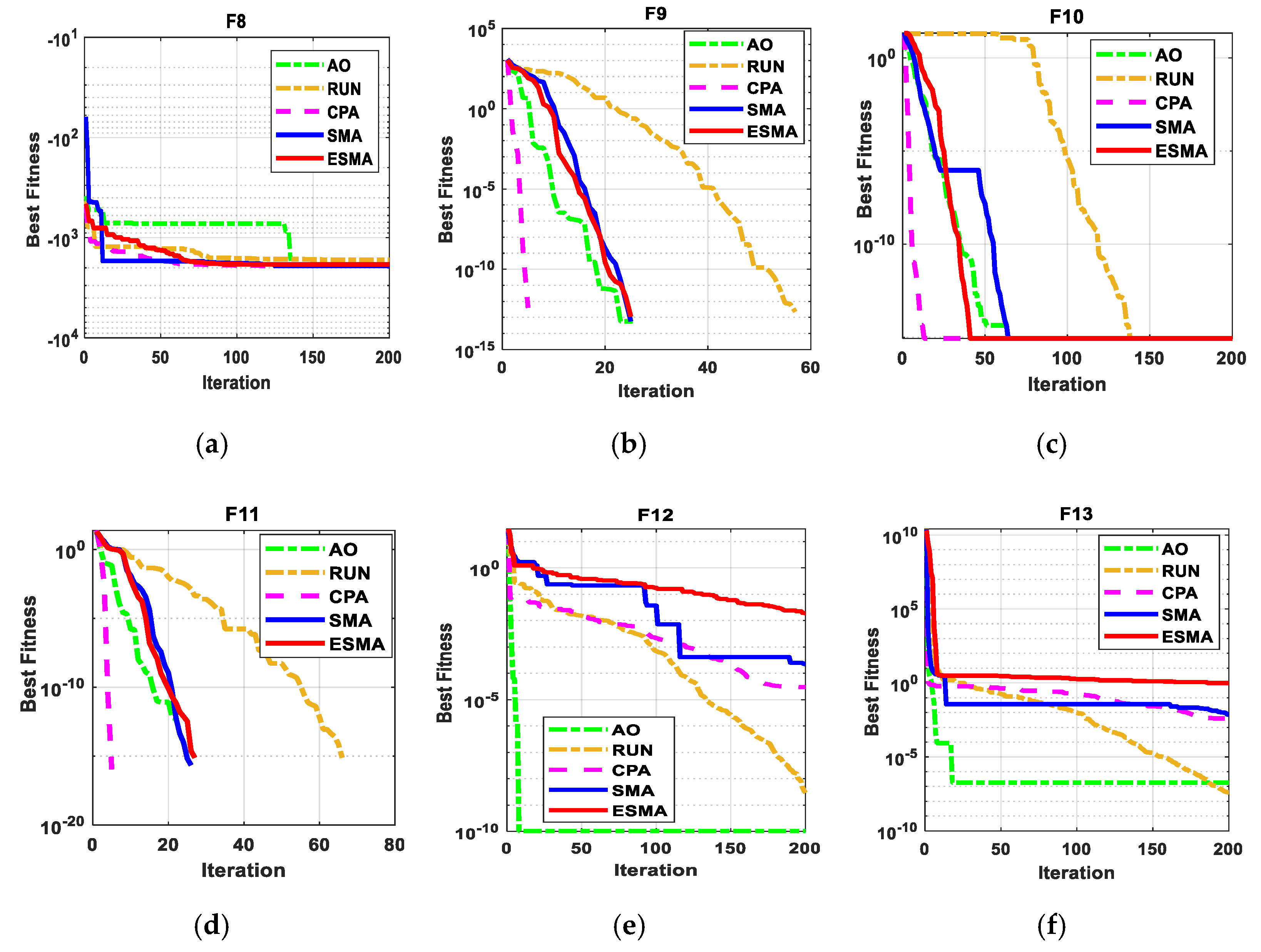
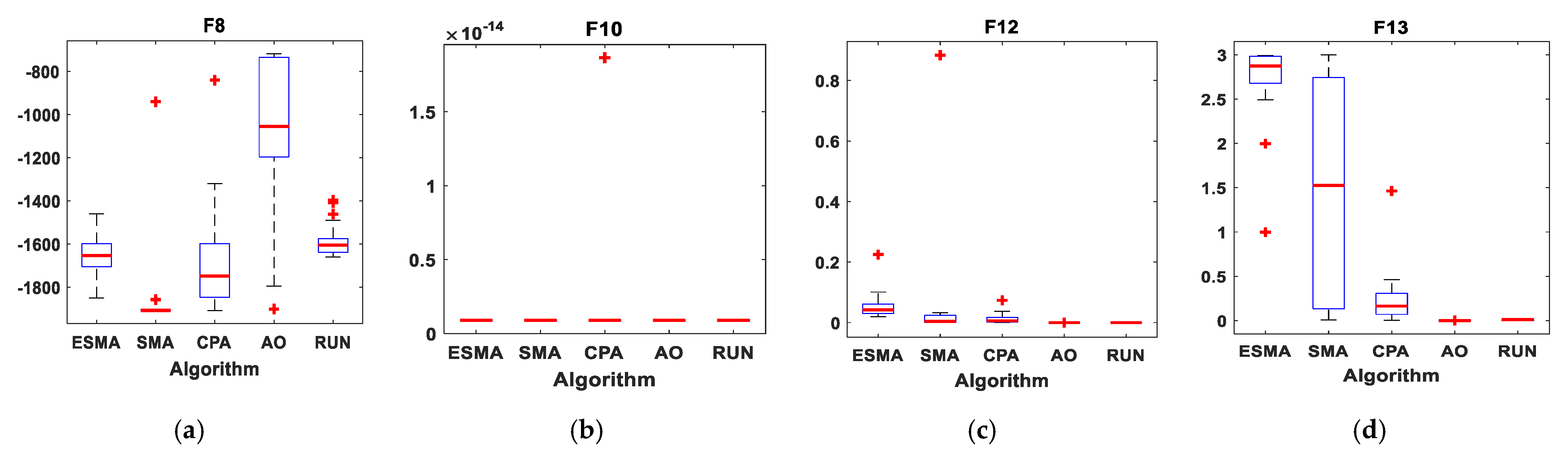
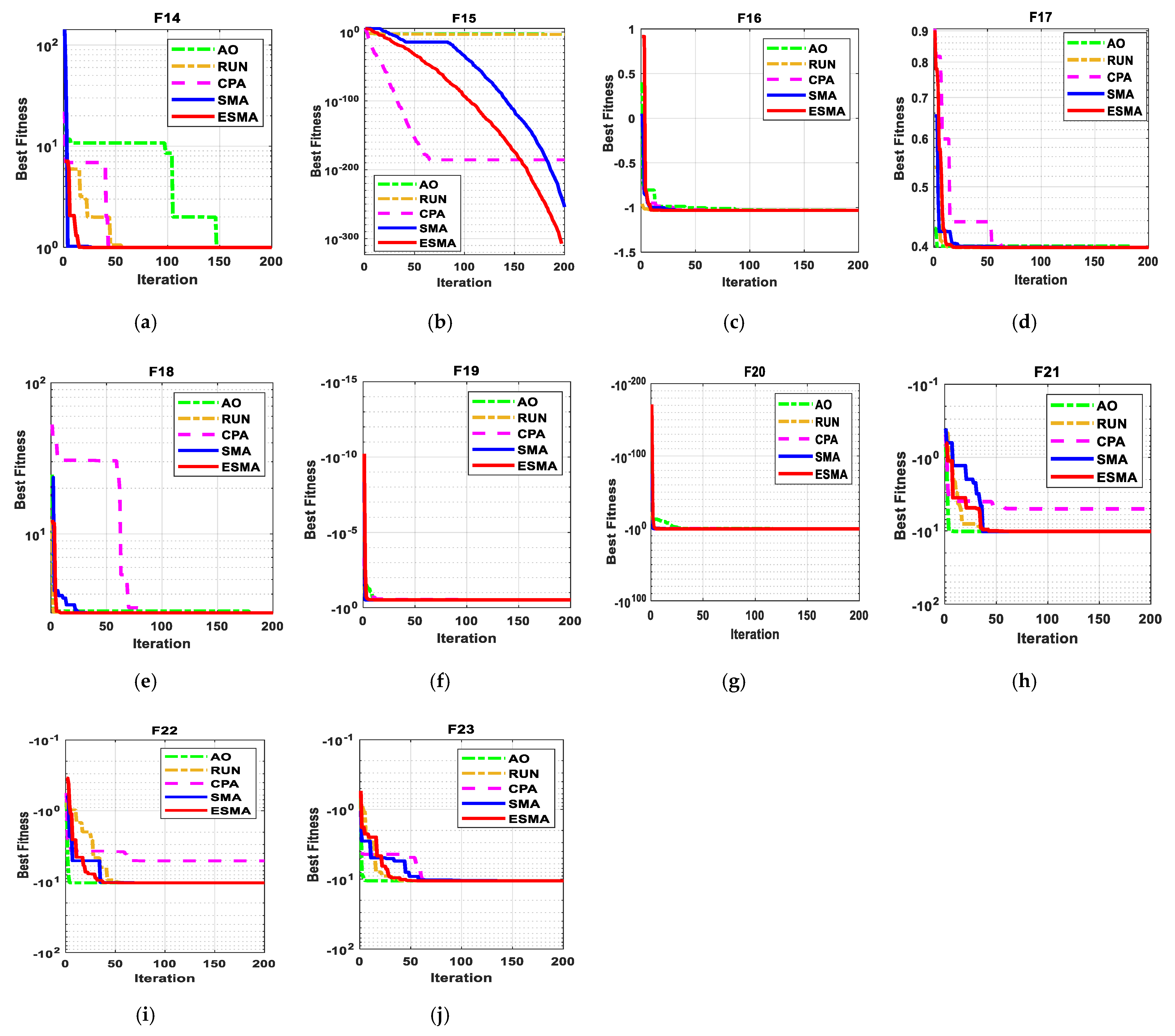
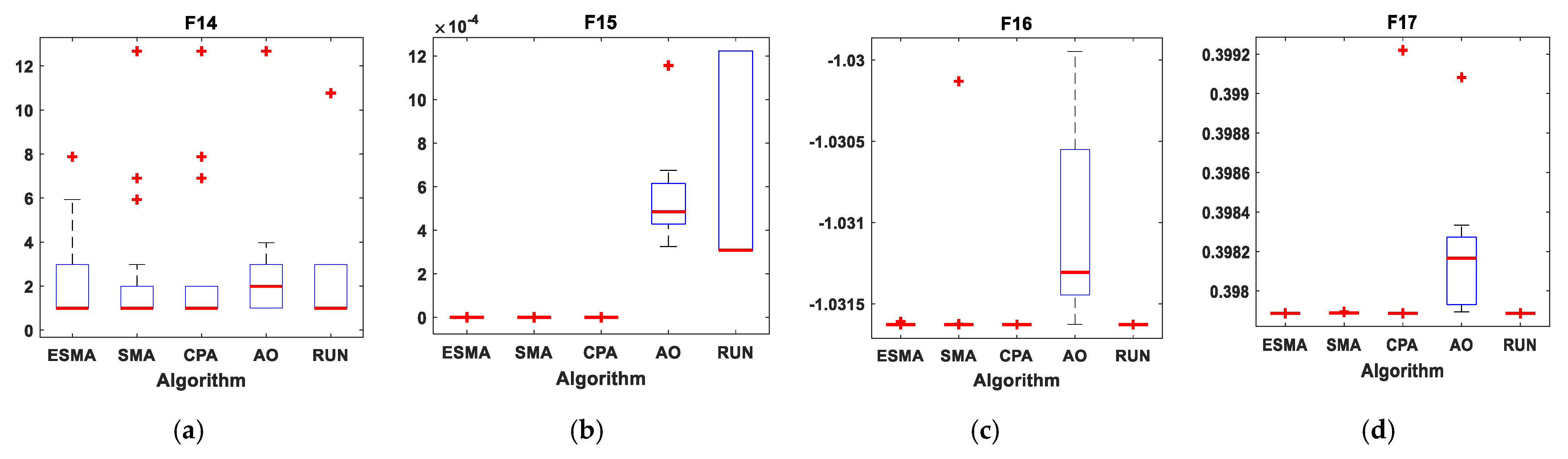
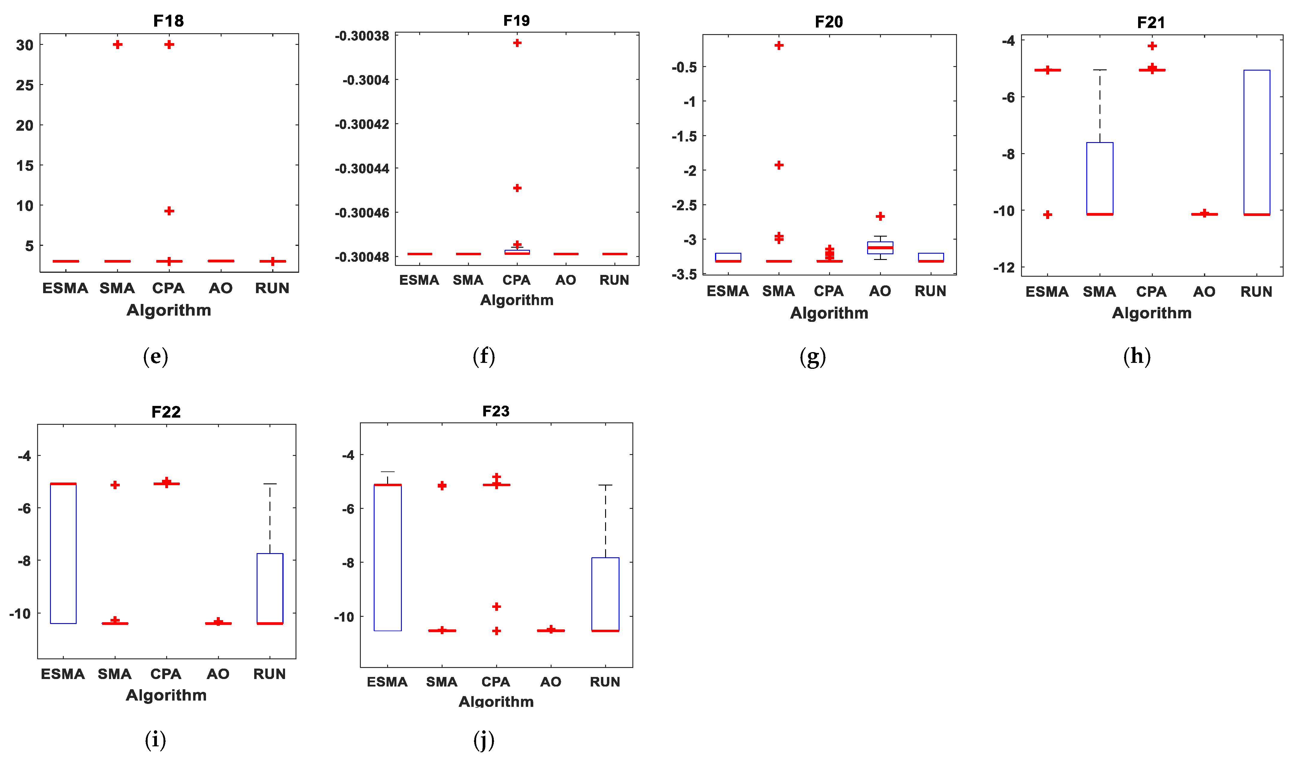
The statistical results of the proposed ESMA algorithm, the original SMA algorithm, and three recent algorithms when applied for unimodal benchmark functions, multimodal benchmark functions, and composite benchmark functions are presented in Table 4, Table 5 and Table 6, respectively. The best values were achieved with the proposed ESMA, SMA, CPA, AO, and RUN algorithms shown in bold. It is obviously seen that the ESMA algorithm reaches to the best solution for many benchmark functions. The convergence curves of all algorithms for the unimodal benchmark functions are shown in Figure 7 while the boxplots for these techniques for this type of functions are displayed in Figure 8. In addition, Figure 9 shows the convergence curves of these algorithms for the multimodal benchmark functions while Figure 10 presents the boxplots for each algorithm for these functions. Finally, the convergence curves of all algorithms for the composite benchmark functions are displayed in Figure 11 while the boxplots for all algorithms for this type of benchmark functions are presented Figure 12. From these figures, it is clearly seen that the proposed ESMA technique reaches a stable point for all functions and the boxplots of the ESMA technique are very narrow for most functions compared to the other well known techniques.
Table 4.
The statistical results of unimodal benchmark functions using the proposed ESMA algorithm and other recent algorithms 1.
Table 5.
The statistical Results of multimodal benchmark functions using the proposed ESMA algorithm and other recent algorithms 1.
Table 6.
The statistical results of composite benchmark functions using the proposed ESMA algorithm and other recent algorithms 1.
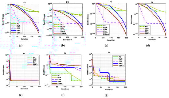
Figure 7.
The convergence curve of all algorithms for seven unimodal benchmark functions. (a) F1; (b) F2; (c) F3; (d) F4; (e) F5; (f) F6; (g) F7.
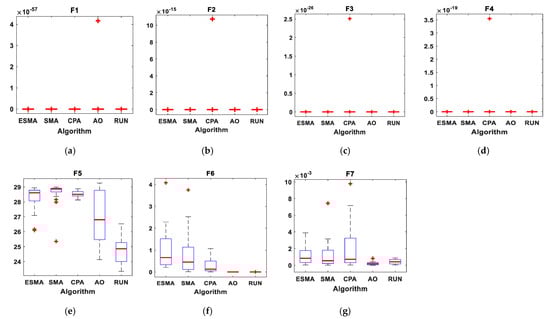
Figure 8.
Boxplots for all algorithms for seven unimodal benchmark functions. (a) F1; (b) F2; (c) F3; (d) F4; (e) F5; (f) F6; (g) F7.
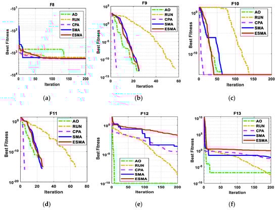
Figure 9.
The convergence curves of all algorithms for six multi-modal benchmark functions. (a) F8; (b) F9; (c) F10; (d) F11; (e) F12; (f) F13.
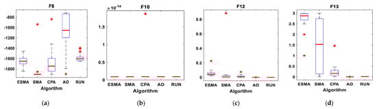
Figure 10.
Boxplots for all algorithms for some of multi-modal benchmark functions. (a) F8; (b) F10; (c) F12; (d) F13.
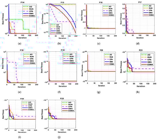
Figure 11.
The convergence curves of all algorithms for ten composite benchmark functions. (a) F14; (b) F15; (c) F16; (d) F17; (e) F18; (f) F19; (g) F20; (h) F21; (i) F22; (j) F23.
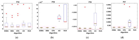
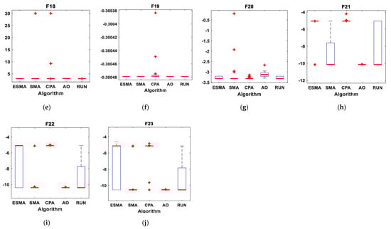
Figure 12.
Boxplots for all algorithms for ten composite benchmark functions. (a) F14; (b) F15; (c) F16; (d) F17; (e) F18; (f) F19; (g) F20; (h) F21; (i) F22; (j) F23.
5.2. Real-World Application
In this subsection, several case studies are implemented on the modified IEEE-30 bus power system to solve the OPF problem. The results of applying the enhanced ESMA for all cases are provided and explained. Conventional SMA and two different optimization algorithms, BWOA and MSA, are also applied to confirm the validity of ESMA.
The case studies are organized as follows: Cases 1 and 2 are dedicated to minimizing the total generation cost without and with carbon tax respectively, Cases 3 and 4 are performed for studying the impact of reserve and penalty cost variation on the optimized cost respectively, Case 5 is implemented for studying of ramp rate effect of TPGs, and finally, Case 6 is performed for studying the impact of load demand uncertainties.
The simulation of optimization techniques is performed based on MATLAB using a computer with the following properties: Intel® Core™ i3-380M Processor 3M Cache, 2.53 GHz and 4 GB RAM.
In every case, the objective function reaches its optimum value after running the algorithm 5 times, and a maximum of 1000 iterations are set as the ending criteria of the algorithms. The settings of control variables are also listed.
5.2.1. Case 1: Minimization of Generation Cost
This case is performed to optimize scheduled output powers from all different types of energy sources used in the modified power system to reach the possible minimum value of the total power cost based on (11).
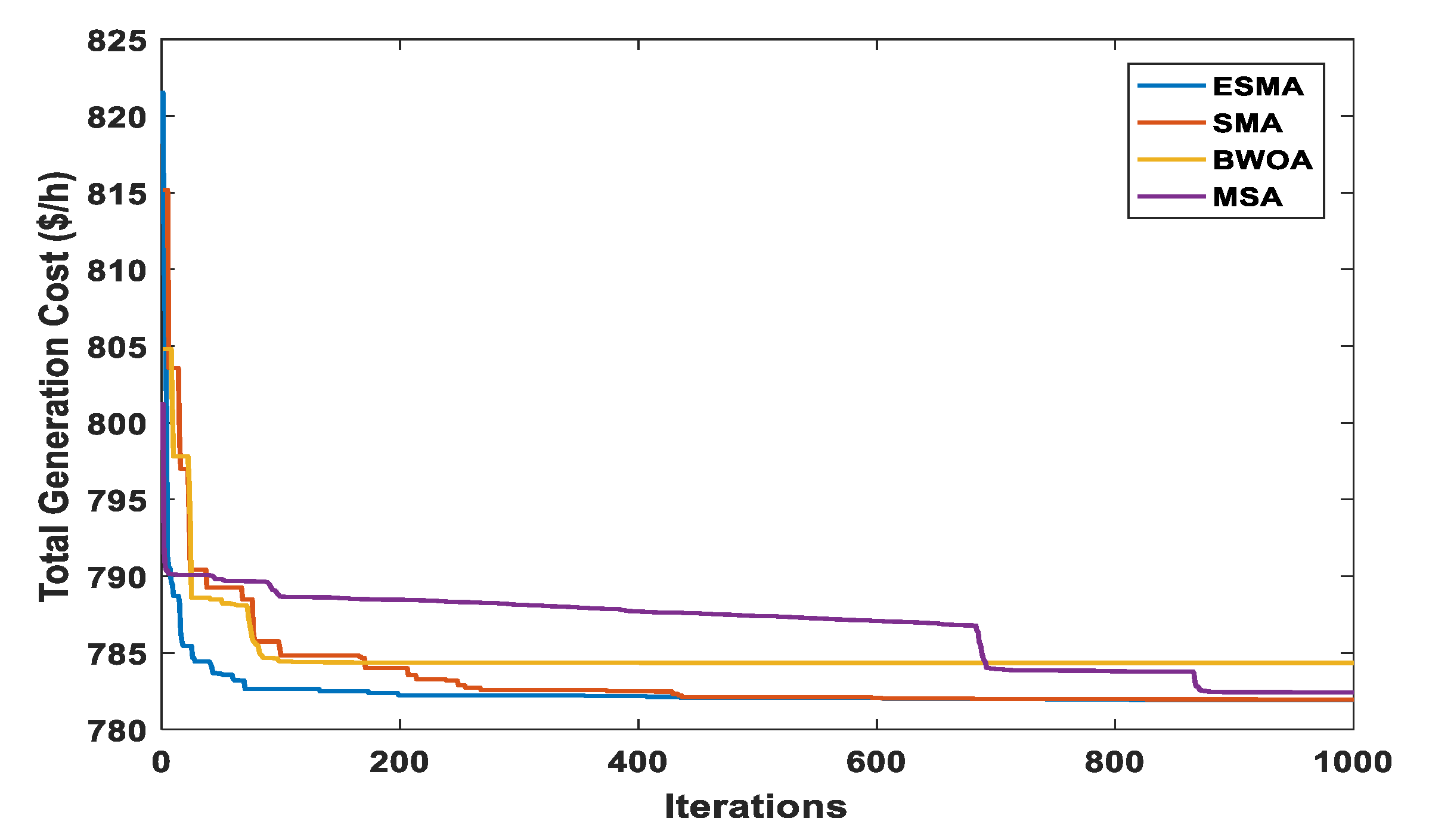
Figure 13 provides the convergences of applied OPF optimization techniques. The optimally obtained results of overall cost, control variables, reactive powers, and other parameters have been provided in Table 7.
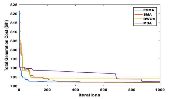
Figure 13.
Characteristics of convergence for different algorithms (Case 1).
Table 7.
Case 1 simulation results.
The voltage of ith bus is denoted by in Table 7. The effectiveness of ESMA is very clear from the simulation results of case 1. Comparing to the conventional SMA and other performed optimization techniques for OPF, ESMA has a fast convergence and better solution quality. Among all applied algorithms, ESMA achieved the minimum total power cost of 781.9376 $/h.
5.2.2. Case 2: Total Power Cost Minimization with Carbon Tax
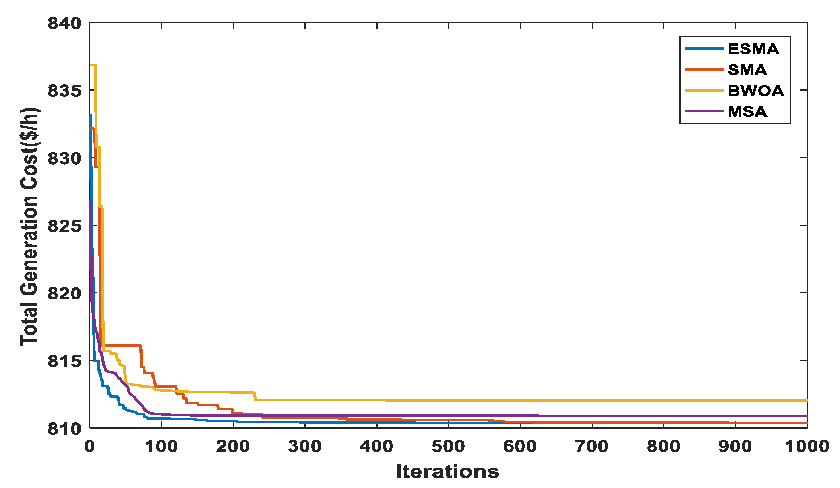
The objective of this case is to minimize the total power cost, with imposing a fixed carbon tax (Ctax) on the thermal power generators because of their CO2 emissions according to (12). The forced Ctax is supposed to be 20 ($/ton) [7]. Increasing the penetration level of wind and solar energy into the power grid is expected with forcing the carbon tax; this conception obviously appears in the simulation results. Similarly to Case 1, a comparison between the convergence of ESMA and other performed algorithms is provided through Figure 14, and the optimally obtained results of overall cost, control variables, reactive powers, and other parameters have been provided in Table 8.
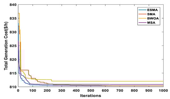
Figure 14.
Characteristics of convergence for different algorithms (Case 2).
Table 8.
Case 2 simulation results.
The minimum value of total power cost achieved by ESMA is 810.3558 $/h which means that ESMA outdoes SMA and all other used techniques with regard to total power cost minimization and the convergence of the solution.
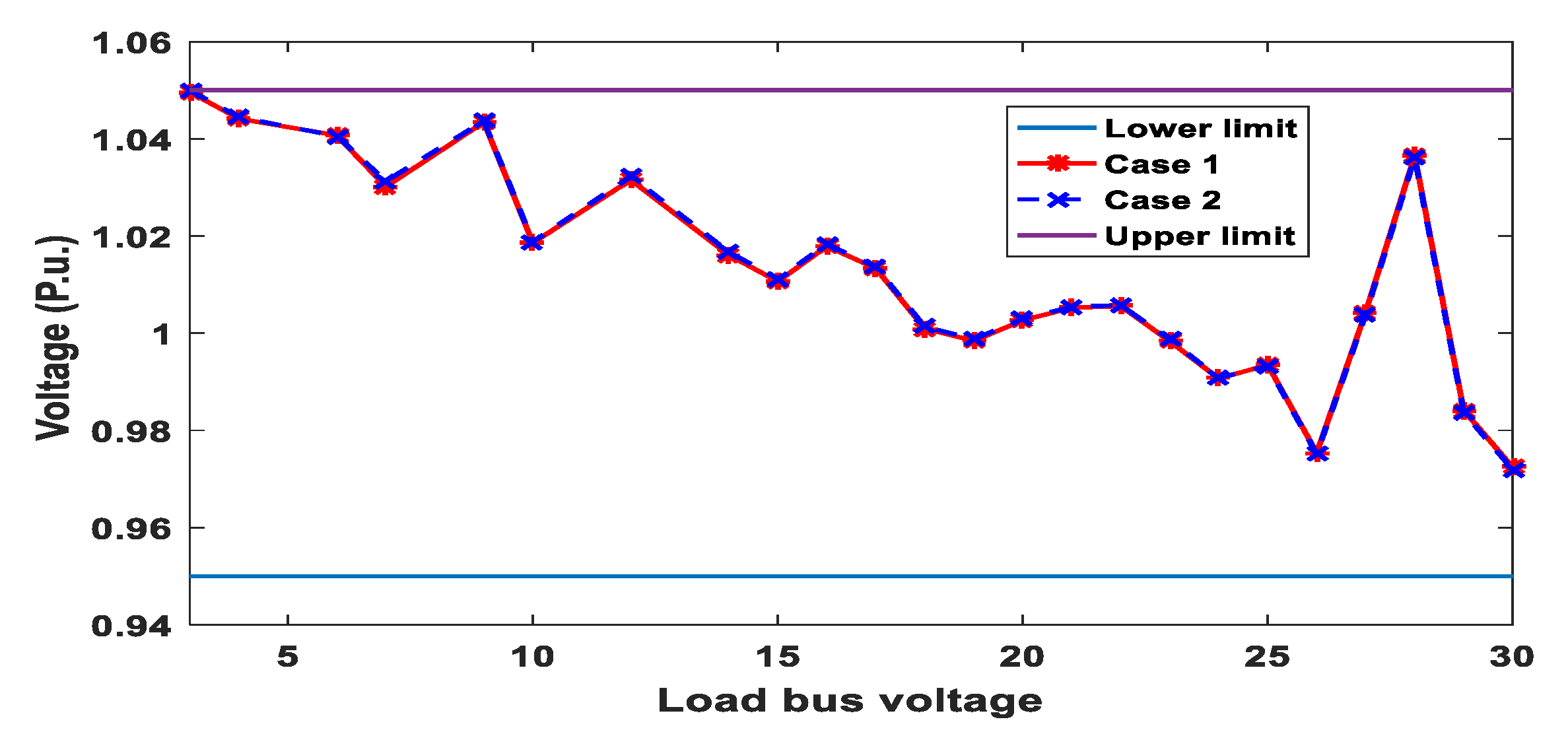
Load buses voltages have an important role in OPF study. Therefore, it is essential to deal with the constraints of load buses voltages. Operating voltages of all load buses in the IEEE- 30 bus system must be within the range [0.95–1.05] p.u.
In this concern, Figure 15 provides voltage profiles of load buses for Case 1 and Case 2. It is clear from Figure 15 that all voltages of load buses are inside limits after finishing the optimization process of the two cases.
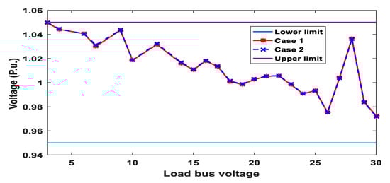
Figure 15.
Profile voltages of Load buses for Cases 1 and 2.
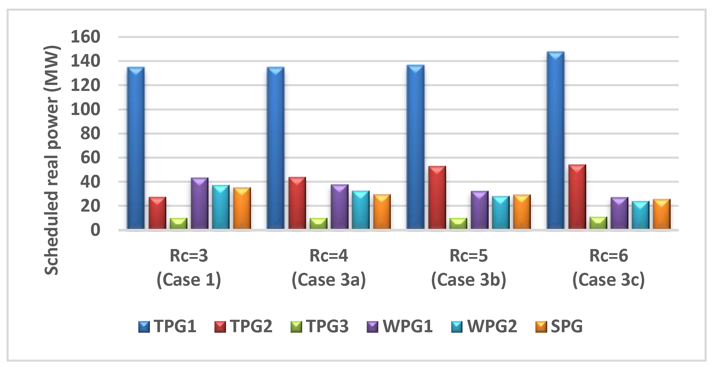
5.2.3. Case 3: Impact of Reserve Cost Variation on the Optimized Cost
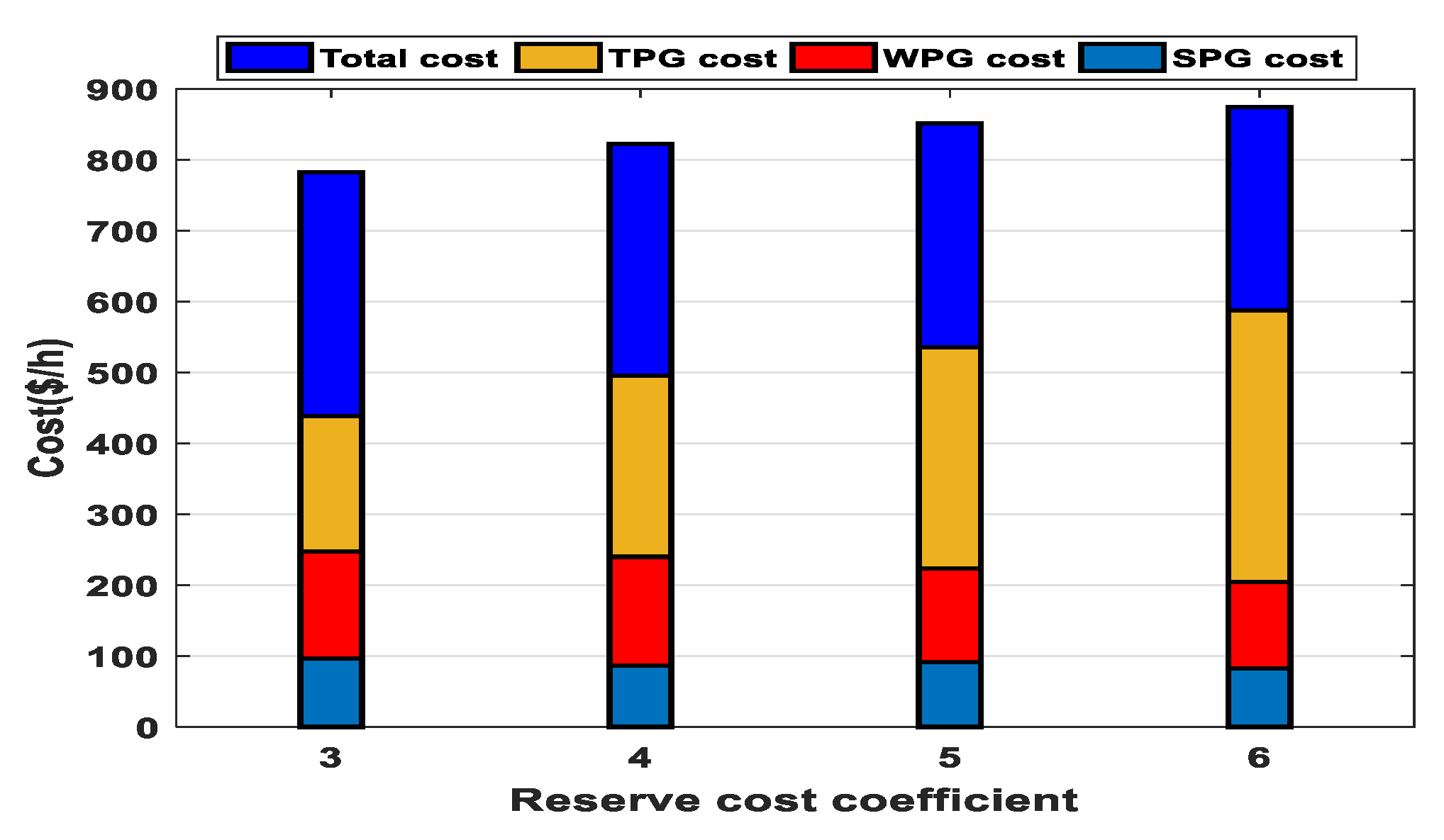
This case is applied to study and analyze the impact of variation of reserve cost coefficient on various optimized costs. All relevant parameters were kept as those used in Case 1 except reserve cost coefficients. In this case, SPG and WPGs have reserve cost coefficients started from (Case 1) to until with an increase of 1, and their penalty cost coefficients are as the same values used in Case 1. The optimally scheduled powers of all generators are shown in Figure 16. To make Figure 16 clearer, Case 3a denotes , Case 3b denotes , while Case 3c denotes . The optimally scheduled powers from WPGs and SPG decrease with the increase in reserve cost coefficient as reducing the scheduled power requests a smaller quantity from the spinning reserve. When there is a shortage of output power from WPGs or SPG, TPGs compensate it. Therefore, the cost of TPGs rises as noticed from the cost profile of TPGs in Figure 17 while the costs of WPGs and SPG decreases gradually to a certain amount. In total, the entire cost of the produced power rises with the rise in the reserve cost coefficient.
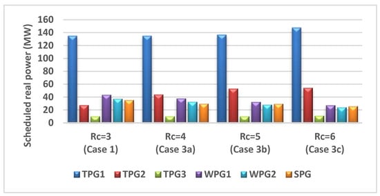
Figure 16.
Impact of reserve cost coefficient (Rc) variation on the optimally scheduled active powers.
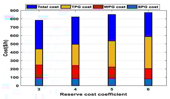
Figure 17.
Impact of Rc variation on costs of all generators.
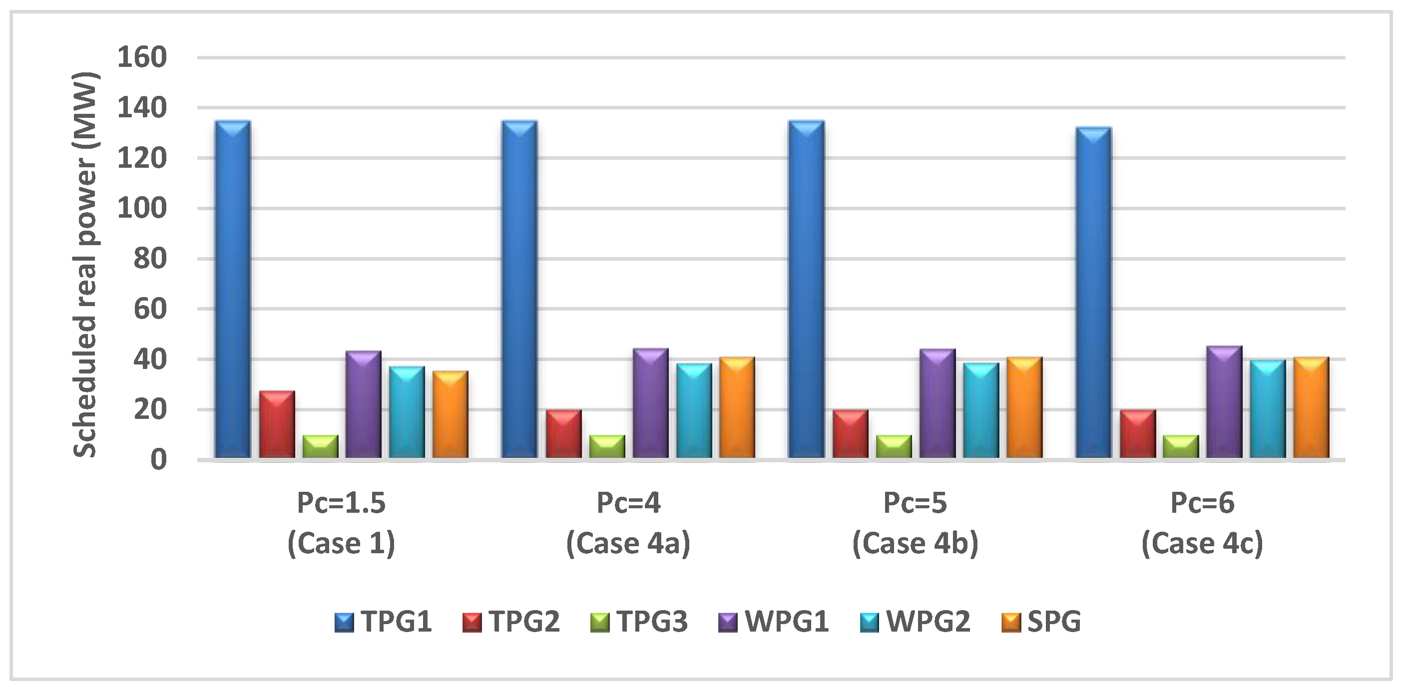
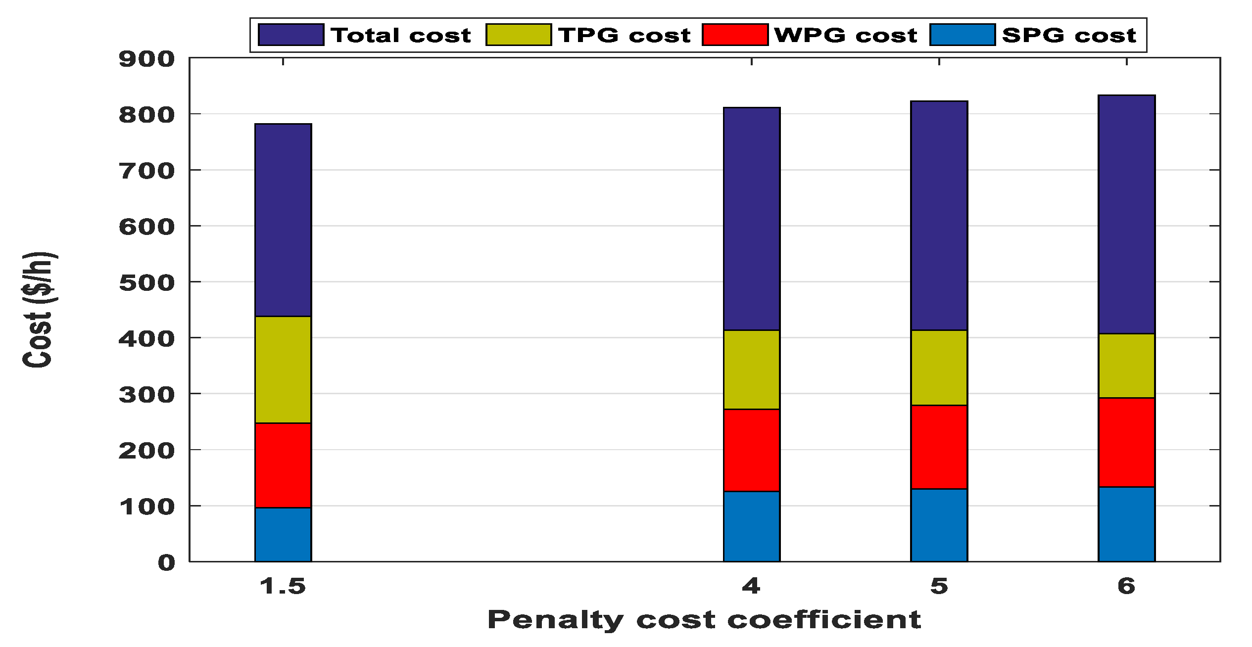
5.2.4. Case 4: Impact of Penalty Cost Variation on the Optimized Cost
The effect of varying the penalty cost coefficient on various optimized costs is studied and analyzed in this case. All relevant parameters were kept as those used for Case 1 except the penalty cost coefficients. In this case, SPG and WPGs have coefficients of penalty cost started from (Case 1) to (Case 4a), (Case 4b), and (Case 4c), while reserve cost coefficients remain unchanged from Case 1, . Figure 18 illustrates the optimally scheduled power from all generators.
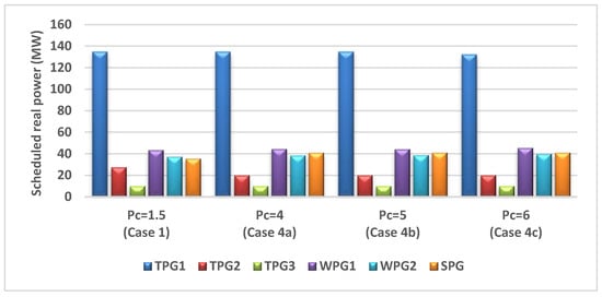
Figure 18.
Impact of penalty cost coefficient (Pc) variation on the optimally scheduled active power.
If the penalty cost coefficient rises, the scheduled output powers of WPGs and SPG will increase because the rise in the scheduled output power will help to decrease the penalty cost in case of wind speed or solar irradiance has a high value. This concept is unlike the concept in the previous case because the raises in the scheduled output powers do not sound identical for all RESs due to the extremely non-linear relationships between PDFs and penalty or reserve cost of RESs. From Figure 19, a progressive increment in WPGs cost and a minor fluctuation in the SPG cost are observed. It is also noticed that the cost of TPGs is approximately constant in addition to a steady growth in total power cost.
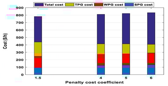
Figure 19.
Impact of Pc variation on costs of all generators.
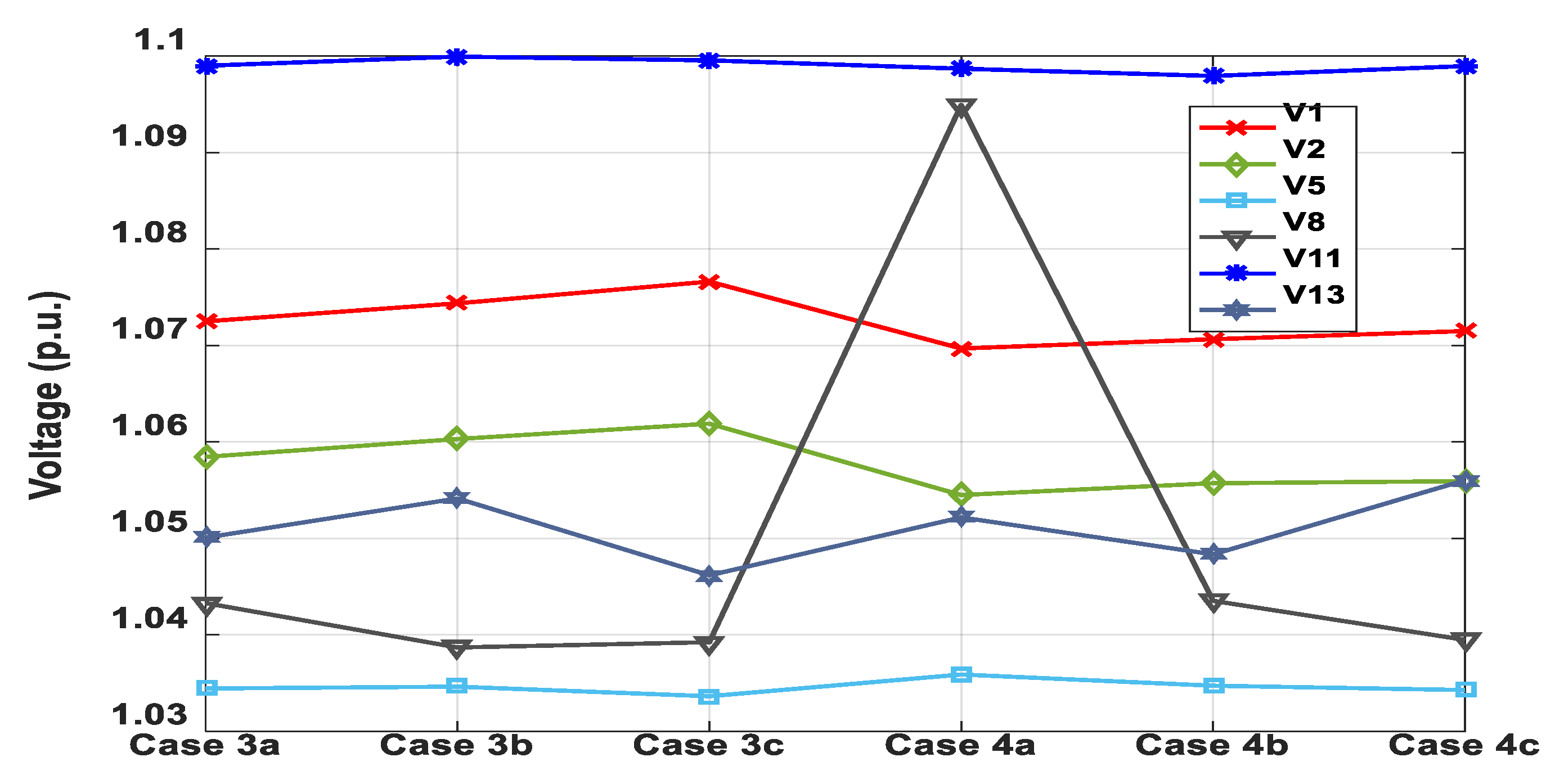
All generator buses voltages for Cases 3 and 4 are presented in Figure 20. It is noticed that all generator buses voltages lie on the specified range of p.u. voltage (0.95–1.1). The generators’ reactive powers are also illustrated in Figure 21. The reactive power limits mentioned in Table 7 indicate that TPG3 and WPG2 reached their reactive power capability maximum limits for many cases. Accordingly, considering the reactive power constraints when performing any optimization technique is very important.
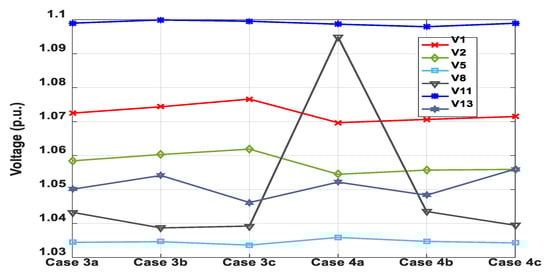
Figure 20.
Generator buses voltages (Cases 3 and 4).
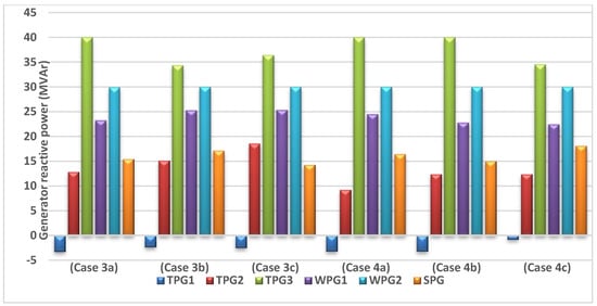
Figure 21.
Scheduled reactive powers for all generators (Cases 3 and 4).
5.2.5. Case 5: The Impact of Considering Ramp-Rate Limits of TPGs
The impact of considering ramp rate limits of TPGs while minimizing the total power cost based on (11) is studied and analyzed in this case. The produced power at the preceding hour for TPGs and their limits of ramp-rate are provided in Table 1 [36].
Table 9 provides the optimal results of this case such as total power cost, control variables, reactive powers, and other important parameters.
Table 9.
Case 5 simulation results (considering the effect of ramp rate).
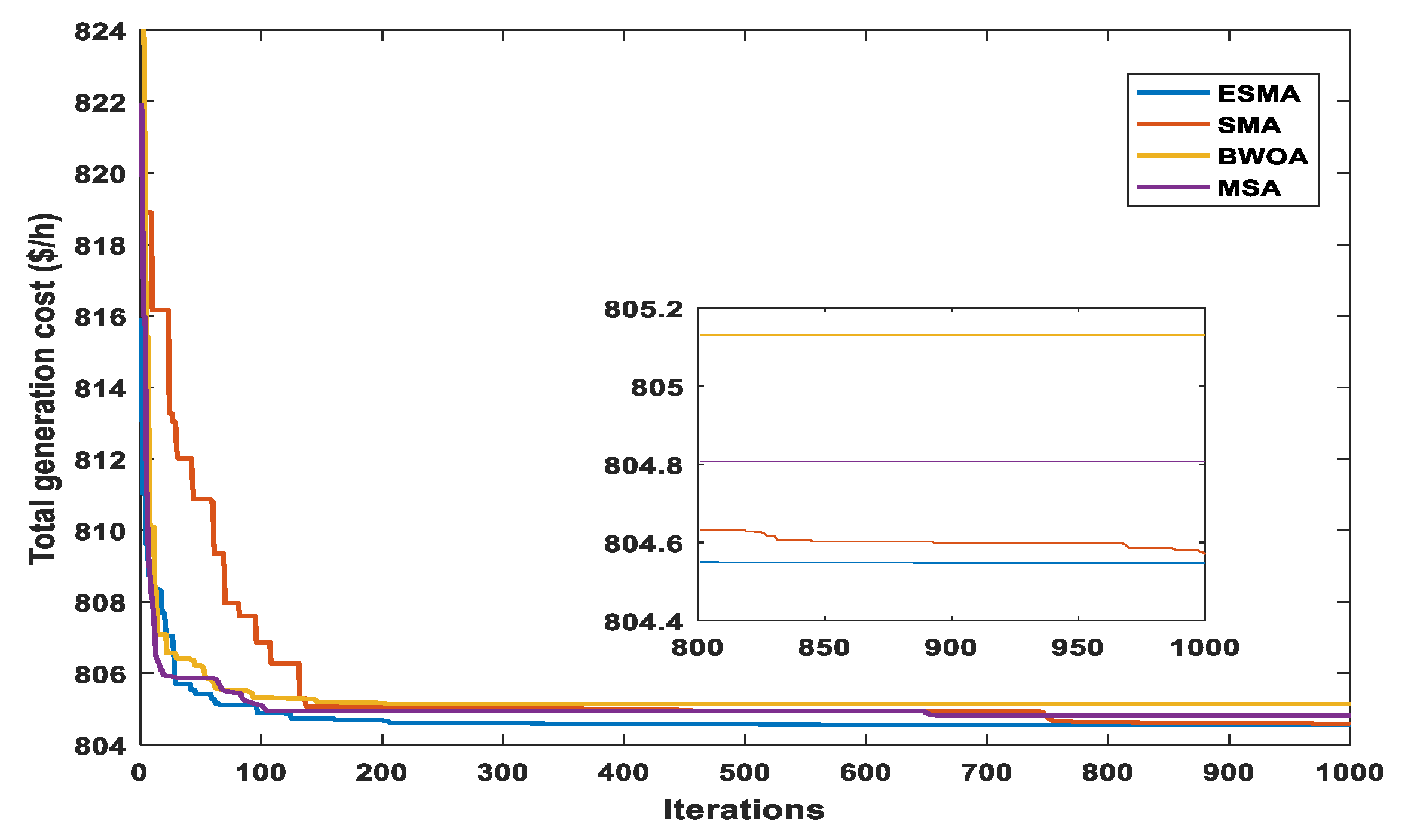
Figure 22 provides the convergences of the different applied techniques in Case 5.
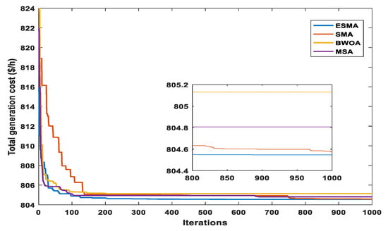
Figure 22.
Solution convergence of different algorithms (Case 5).
The impact of the ramp rate limits of the TPGs is clear from the Case 5 simulation results. If we look at the results of Case 5 in Table 9 and the results of Case 1 in Table 7, we can find that the total power cost is increased as expected as a result of changing the new operating points of TPGs from their original operating points without ramp rate constraints. The effectiveness of ESMA is very clear from the simulation results of Case 5. Compared to the conventional SMA and other applied optimization algorithms, ESMA has the fastest convergence and the best solution quality. The minimum overall power cost achieved using the ESMA is 804.5476 $/h. Thus, ESMA outperforms SMA and all other performed techniques with regard to total power cost minimization and the convergence of solutions for this practical case. There is no violation in system constraints after performing the OPF study as shown in Table 9.
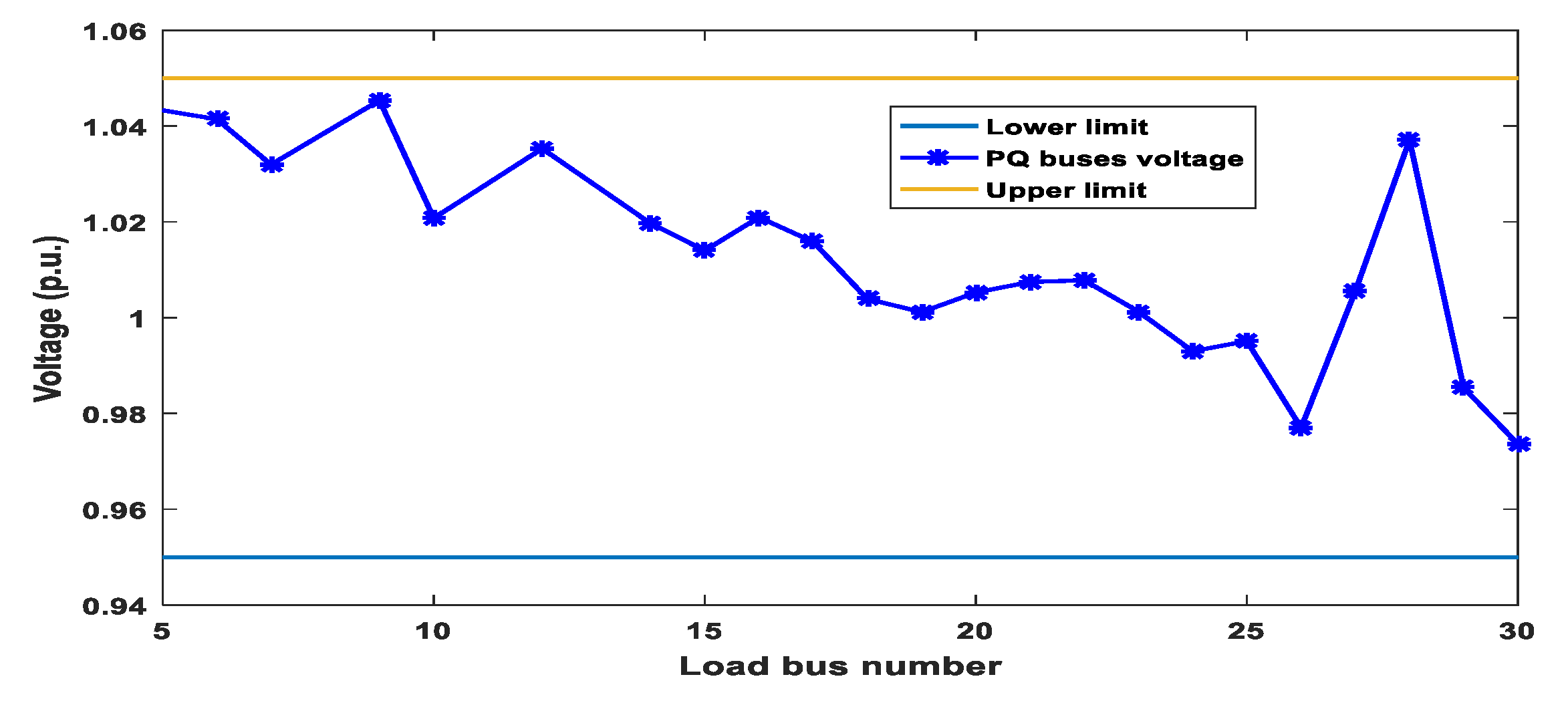
Figure 23 shows also the voltage profile of load buses in Case 5. It is noticed that all voltages of load buses are inside the predefined limits.
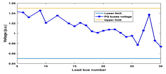
Figure 23.
Profile of PQ buses voltages (Case 5).
5.2.6. Case 6: The Impact of Load Demand Uncertainties
In Case 6, another realistic situation of load demand variation is provided. The load demand uncertainty has been modeled by the normal PDF [37]. A level-based procedure is executed to accomplish the process of optimization during some different levels (scenarios) of the power system load.
The uncertainty of the load using the normal PDF with standard deviation (σd) = 10 and mean (μd) = 70 is illustrated in Figure 24. There are four-color areas in Figure 24. These areas denote the four considered levels of load demand (Pd).
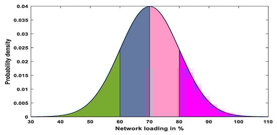
Figure 24.
Representation of load uncertainty by normal PDF (μd = 70, and σd = 10).
The occurring probability of the i-th level of load demand () is depicted below [12]:
Equation (51) determines the mean of the i-th level of load demand ().
The calculated values of the four means, as a percentage of nominal loading, and the four probabilities for the four loading levels are recorded in Table 10. For each scenario, the four performed algorithms try to optimally minimize the total power cost based on (11). In each loading scenario, the scheduled powers of all the system generators are optimized.
Table 10.
Probabilities and means of loading levels [12].
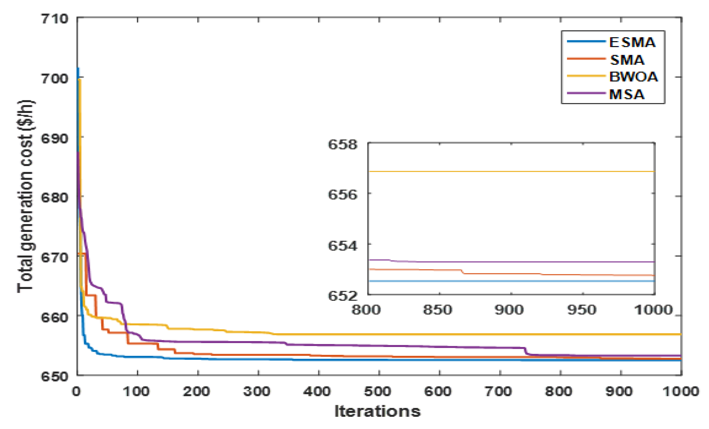
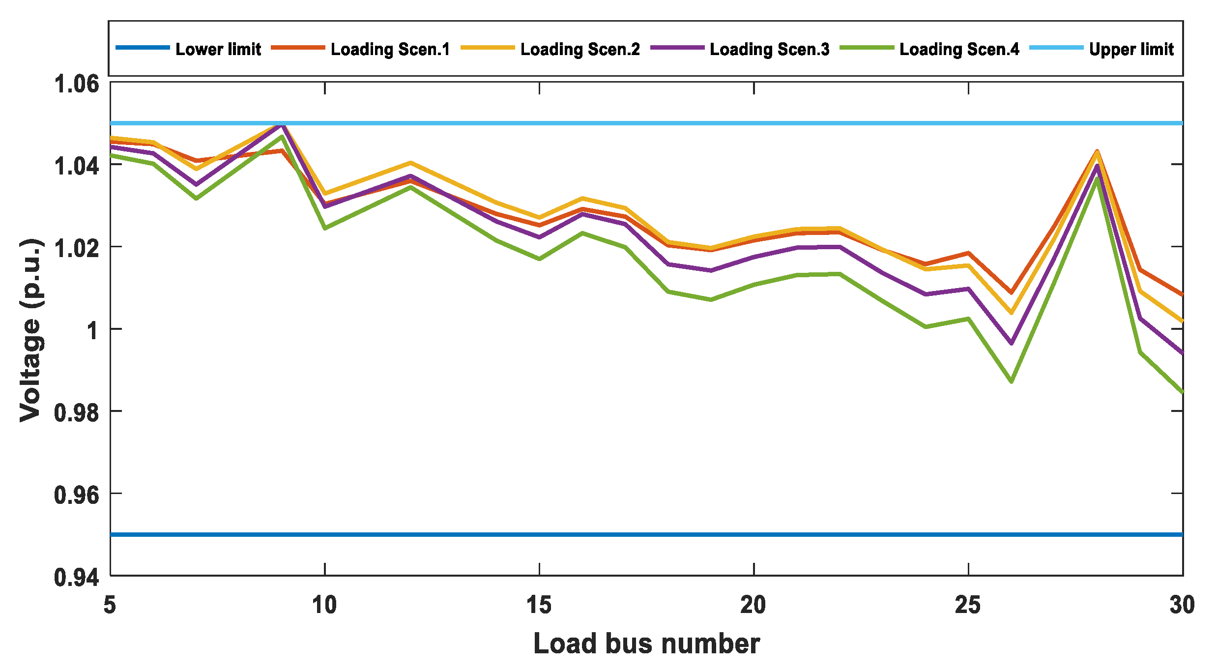
For simplicity, only the results of loading levels 1 and 3 (L1 and L3) are recorded in Table 11 and Table 12. It is clear from the results of Case 6 that the operation cost and power losses of the system under realistic loading levels are justifiably lesser than their values under theoretical conditions in Case 1. Figure 25 illustrates that ESMA outdoes all other performed methods with regard to overall power cost minimization and the convergence of solution. The voltage profiles of load buses for different loading levels for the ESMA are plotted in Figure 26. The values of voltage and system variables are recorded in Table 11 and Table 12. These values show that all system constraints are satisfied.
Table 11.
Case 6 simulation results (L1).
Table 12.
Case 6 simulation results (L3).
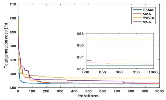
Figure 25.
Solution convergence for various algorithms (Case 6).
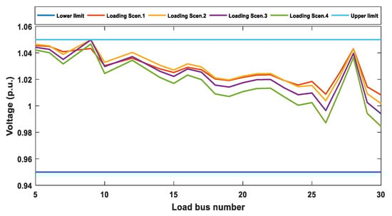
Figure 26.
Profiles of load buses voltages for all system loading levels (Case 6).
6. Conclusions
This research provided an enhanced slime mould algorithm to solve optimally the OPF problem. The performance of the proposed algorithm has been evaluated using 23 benchmark test functions and has been compared with the conventional SMA and three recent optimization algorithms: CPA, AO, and RUN. The results of the proposed ESMA algorithm are compared with these well-known optimization algorithms. The ESMA algorithm reached the best solution for many benchmark functions.
Consequently, the ESMA was used to solve the OPF problem in the IEEE-30 bus power system that modified to include stochastic solar and wind energy sources. The uncertain outputs of solar and wind energy sources were modelled through lognormal and Weibull PDFs, respectively.
The total cost of power produced from all power generators was optimally minimized in two different case studies; one of them neglected the carbon emission and the other considered it. The effect of varying the reserve and penalty cost coefficients of SPG and WPGs on the total power cost were also analyzed.
The impacts of considering ramp rate limits of TPGs and uncertain load demand have been studied to observe the validity of ESMA under more practical cases.
To test ESMA validity in real world applications, conventional SMA and two other optimization techniques, BWOA and MSA, were performed for the adjusted IEEE-30 bus system at the same system conditions. Simulation results obtained by the ESMA in each case study were compared with the results obtained by other applied algorithms.
Simulation results of all case studies prove the effectiveness of ESMA for solving of OPF problem with maintaining the system constraints inside the limits that have been set by the ISO. ESMA outperforms the conventional SMA and other optimization algorithms in terms of total power cost minimization and the convergence of problem solution under the practical and theoretical cases.
Author Contributions
Conceptualization, M.F., S.K. and A.M.A. (Ahmed M. Atallah); Data curation, M.H.H. and A.M.A. (Ahmed M. Agwa); Formal analysis, M.F., S.K. and A.M.A. (Ahmed M. Atallah); Software, M.H.H. and A.M.A. (Ahmed M. Agwa); Investigation, M.F., S.K. and A.M.A. (Ahmed M. Atallah); Methodology, M.F., S.K. and A.M.A. (Ahmed M. Atallah); Project administration, M.H.H. and A.M.A. (Ahmed M. Agwa); Resources, M.H.H. and A.M.A. (Ahmed M. Agwa); Software M.F., S.K. and A.M.A. (Ahmed M. Atallah); Supervision, S.K., M.H.H. and A.M.A. (Ahmed M. Agwa); Validation, S.K. and M.F.; Visualization, M.H.H. and A.M.A. (Ahmed M. Agwa); Writing original draft, M.F., S.K. and A.M.A. (Ahmed M. Atallah); Writing—review & editing, M.H.H. and A.M.A. (Ahmed M. Agwa). All authors have read and agreed to the published version of the manuscript.
Funding
This research was funded by the Deputyship for Research & Innovation, Ministry of Education in Saudi Arabia through the project number “IF_2020_NBU_405”.
Institutional Review Board Statement
Not applicable.
Informed Consent Statement
Not applicable.
Data Availability Statement
Not applicable.
Acknowledgments
The authors extend their appreciation to the Deputyship for Research & Innovation, Ministry of Education in Saudi Arabia for funding this research work through the project number “IF_2020_NBU_405”. The authors gratefully thank the Prince Faisal bin Khalid bin Sultan Research Chair in Renewable Energy Studies and Applications (PFCRE) at Northern Border University for their support and assistance.
Conflicts of Interest
The authors declare no conflict of interest.
Nomenclature
| The fossil fuel cost | |
| ai, bi, and ci | Coefficients of cost for the ith TPG |
| PTPG,i | Output power from the ith TPG |
| NTPG | The number of TPGs in the power system |
| di and | Coefficients of valve-point loading |
| The minimum power of ith TPG | |
| The direct cost of wind power produced from the jth WPG | |
| Scheduled output power from the jth WPG | |
| The direct cost coefficient of the jth WPG | |
| The direct cost of the kth SPG | |
| Scheduled output power from the kth SPG | |
| The coefficient of direct cost associated with the kth SPG | |
| The reserve cost for the jth WPG | |
| The available power of the jth WPG | |
| Coefficient of reserve cost for the jth WPG | |
| Available output power from the jth WPG | |
| The Weibull PDF of the jth WPG output power | |
| Penalty cost for the jth WPG | |
| Coefficient of penalty cost for the jth WPG | |
| The rated output power of the jth WPG | |
| The reserve cost for the kth SPG | |
| Available output power from the kth SPG | |
| Coefficient of reserve cost for the kth SPG | |
| The shortage occurrence probability of solar power | |
| The expectation of being the output of SPG below the | |
| Coefficient of penalty cost of the kth SPG | |
| The surplus occurrence probability of solar power | |
| ) | The expectation of being the output of SPG above the |
| The coefficients of emissions from the ith TPG | |
| The emission cost | |
| Carbon tax | |
| Emissions (ton/h) | |
| Output power from the ith TPG at previous hour | |
| Limits of down and up ramp-rate for the ith TPG | |
| NSPG and NWPG | The number of SPGs and WPGs existing in the modified power system, respectively |
| NB | The total number of grid buses |
| The difference between voltage angles of bus i and bus j | |
| The active and reactive components of the generated power at bus i, respectively | |
| The active and reactive components of load demand at bus i, respectively | |
| The conductance and susceptance between bus i and bus j, respectively | |
| NG | The total number of generators in the system |
| NB | The total number of load buses |
| NL | The total number of system transmission lines |
| and c | Shape and scale factors of Weibull PDF, respectively |
| Vd | Voltage deviation |
| I | Solar irradiance (W/m2) |
| The cut-in, cut-out, and rated wind speeds of the wind turbine, respectively | |
| The rated power of wind turbine | |
| The solar irradiance in a standard environment (800 W/m2) | |
| Specific irradiance amount (120 W/m2) | |
| The rated power of SPG | |
| Value reduces linearly from one to zero | |
| T | The t-th iteration |
| The individual position that has the most focus on smell found currently | |
| The slime mould position | |
| and | Two individuals selected randomly from the whole population |
| S(i) | The fitness value of , i ∈ 1, 2, 3, …, n |
| R | Random value in range [0, 1] |
| bF and wF | The best and worst fitness obtained in the present iteration |
| SmellIndex | The sequence of sorting the values of fitness function |
| UB and LB | The upper and lower boundaries of the search space, respectively |
| Rand | The random value varies from 0 to 1 |
| Z | Parameter between [0, 0.1] |
| and | The high and low limits of i-th level of load demand, respectively |
References
- Carpentier, J. Contribution to the economic dispatch problem. Bull. Soc. Fr. Electr. 1962, 3, 431–447. [Google Scholar]
- Hussain, S.; Ahmed, M.A.; Kim, Y.C. Efficient Power Management Algorithm Based on Fuzzy Logic Inference for Electric Vehicles Parking Lot. IEEE Access 2019, 7, 65467–65485. [Google Scholar] [CrossRef]
- Hussain, S.; Lee, K.B.; Ahmed, M.A.; Hayes, B.; Kim, Y.C. Two-stage fuzzy logic inference algorithm for maximizing the quality of performance under the operational constraints of power grid in electric vehicle parking lots. Energies 2020, 13, 4634. [Google Scholar] [CrossRef]
- Roy, R.; Jadhav, H.T. Optimal power flow solution of power system incorporating stochastic wind power using Gbest guided artificial bee colony algorithm. Int. J. Electr. Power Energy Syst. 2015, 64, 562–578. [Google Scholar] [CrossRef]
- Panda, A.; Tripathy, M. Security constrained optimal power flow solution of wind-thermal generation system using modified bacteria foraging algorithm. Energy 2015, 93, 816–827. [Google Scholar] [CrossRef]
- Ravi, K. Optimal power flow considering intermittent wind power using particle swarm optimization. Int. J. Renew. Energy Res. 2016, 6, 504–509. [Google Scholar]
- Biswas, P.P.; Suganthan, P.N.; Amaratunga, G.A. Optimal power flow solutions incorporating stochastic wind and solar power. Energy Convers. Manag. 2017, 148, 1194–1207. [Google Scholar] [CrossRef]
- Khan, B.; Singh, P. Optimal power flow techniques under characterization of conventional and renewable energy sources: A comprehensive analysis. J. Eng. 2017, 2017, 9539506. [Google Scholar] [CrossRef] [Green Version]
- Reddy, S.S. Optimal power flow with renewable energy resources including storage. Electr. Eng. 2017, 99, 685–695. [Google Scholar] [CrossRef]
- Shaheen, M.A.; Hasanien, H.M.; Al-Durra, A. Solving of Optimal Power Flow Problem Including Renewable Energy Resources Using HEAP Optimization Algorithm. IEEE Access 2021, 9, 35846–35863. [Google Scholar] [CrossRef]
- Khazali, A.; Kalantar, M. Optimal generation dispatch incorporating wind power and responsive loads: A chance-constrained framework. J. Renew. Sustain. Energy 2015, 7, 023138. [Google Scholar] [CrossRef]
- Biswas, P.P.; Arora, P.; Mallipeddi, R.; Suganthan, P.N.; Panigrahi, B.K. Optimal placement and sizing of FACTS devices for optimal power flow in a wind power integrated electrical network. Neural Comput. Appl. 2021, 33, 6753–6774. [Google Scholar] [CrossRef]
- Chamanbaz, M.; Dabbene, F.; Lagoa, C. AC optimal power flow in the presence of renewable sources and uncertain loads. arXiv 2017, arXiv:1702.02967. [Google Scholar]
- Kaymaz, E.; Duman, S.; Guvenc, U. Optimal power flow solution with stochastic wind power using the Lévy coyote optimization algorithm. Neural Comput. Appl. 2021, 33, 6775–6804. [Google Scholar] [CrossRef]
- Khunkitti, S.; Siritaratiwat, A.; Premrudeepreechacharn, S. Multi-objective optimal power flow problems based on slime mould algorithm. Sustainability 2021, 13, 7448. [Google Scholar] [CrossRef]
- Nusair, K.; Alasali, F.; Hayajneh, A.; Holderbaum, W. Optimal placement of FACTS devices and power-flow solutions for a power network system integrated with stochastic renewable energy resources using new metaheuristic optimization techniques. Int. J. Energy Res. 2021, 45, 18786–18809. [Google Scholar] [CrossRef]
- ElSayed, S.K.; Elattar, E.E. Slime Mold Algorithm for Optimal Reactive Power Dispatch Combining with Renewable Energy Sources. Sustainability 2021, 13, 5831. [Google Scholar] [CrossRef]
- Wei, Y.; Zhou, Y.; Luo, Q.; Deng, W. Optimal reactive power dispatch using an improved slime mould algorithm. Energy Rep. 2021, 7, 8742–8759. [Google Scholar] [CrossRef]
- Li, S.; Chen, H.; Wang, M.; Heidari, A.A.; Mirjalili, S. Slime mould algorithm: A new method for stochastic optimization. Future Gener. Comput. Syst. 2020, 111, 300–323. [Google Scholar] [CrossRef]
- Tu, J.; Chen, H.; Wang, M.; Gandomi, A.H. The Colony Predation Algorithm. J. Bionic Eng. 2021, 18, 674–710. [Google Scholar] [CrossRef]
- Abualigah, L.; Yousri, D.; Abd Elaziz, M.; Ewees, A.A.; Al-qaness, M.A.; Gandomi, A.H. Aquila Optimizer: A novel meta-heuristic optimization Algorithm. Comput. Ind. Eng. 2021, 157, 107250. [Google Scholar] [CrossRef]
- Ahmadianfar, I.; Heidari, A.A.; Gandomi, A.H.; Chu, X.; Chen, H. RUN beyond the metaphor: An efficient optimization algorithm based on Runge Kutta method. Expert Syst. Appl. 2021, 181, 115079. [Google Scholar] [CrossRef]
- Peña-Delgado, A.F.; Peraza-Vázquez, H.; Almazán-Covarrubias, J.H.; Torres-Cruz, N.; García-Vite, P.M.; Morales-Cepeda, A.B.; Ramirez-Arredondo, J.M. A Novel Bio-Inspired Algorithm Applied to Selective Harmonic Elimination in a Three-Phase Eleven-Level Inverter. Math. Probl. Eng. 2020, 2020, 8856040. [Google Scholar] [CrossRef]
- Mohamed, A. Moth Swarm Algorithm (MSA). MATLAB Central File Exchange. 10 September 2021. Available online: https://www.mathworks.com/matlabcentral/fileexchange/57822-moth-swarm-algorithm-msa (accessed on 15 November 2021).
- Chaib, A.E.; Bouchekara, H.R.; Mehasni, R.; Abido, M.A. Optimal power flow with emission and non-smooth cost functions using backtracking search optimization algorithm. Int. J. Electr. Power Energy Syst. 2016, 81, 64–77. [Google Scholar] [CrossRef]
- Chang, T.P. Investigation on frequency distribution of global radiation using different probability density functions. Int. J. Appl. Sci. Eng. 2010, 8, 99–107. [Google Scholar]
- Shi, L.; Wang, C.; Yao, L.; Ni, Y.; Bazargan, M. Optimal power flow solution incorporating wind power. IEEE Syst. J. 2011, 6, 233–241. [Google Scholar] [CrossRef]
- Yao, F.; Dong, Z.Y.; Meng, K.; Xu, Z.; Iu, H.H.; Wong, K.P. Quantum-inspired particle swarm optimization for power system operations considering wind power uncertainty and carbon tax in Australia. IEEE Trans. Ind. Inform. 2012, 8, 880–888. [Google Scholar] [CrossRef]
- Alsac, O.; Stott, B. Optimal load flow with steady-state security. IEEE Trans. Power Appar. Syst. 1974, PAS-93, 745–751. [Google Scholar] [CrossRef] [Green Version]
- IEC I. 61400e1: Wind Turbines Part 1: Design Requirements; International Electrotechnical Commission: Geneva, Switzerland, 2005.
- Reddy, S.S.; Bijwe, P.R.; Abhyankar, A.R. Real-time economic dispatch considering renewable power generation variability and uncertainty over scheduling period. IEEE Syst. J. 2014, 9, 1440–1451. [Google Scholar] [CrossRef]
- Dubey, H.M.; Pandit, M.; Panigrahi, B.K. Hybrid flower pollination algorithm with time-varying fuzzy selection mechanism for wind integrated multi-objective dynamic economic dispatch. Renew. Energy 2015, 83, 188–202. [Google Scholar] [CrossRef]
- Lai, L.L.; Ma, J.T.; Yokoyama, R.; Zhao, M. Improved genetic algorithms for optimal power flow under both normal and contingent operation states. Int. J. Electr. Power Energy Syst. 1997, 19, 287–292. [Google Scholar] [CrossRef]
- Howard, F.L. The life history of Physarum polycephalum. Am. J. Bot. 1931, 18, 116–133. [Google Scholar] [CrossRef]
- Nadimi-Shahraki, M.H.; Taghian, S.; Mirjalili, S. An improved grey wolf optimizer for solving engineering problems. Expert Syst. Appl. 2021, 166, 113917. [Google Scholar] [CrossRef]
- Niknam, T.; Narimani, M.R.; Aghaei, J.; Tabatabaei, S.; Nayeripour, M. Modified honey bee mating optimisation to solve dynamic optimal power flow considering generator constraints. IET Gener. Transm. Distrib. 2011, 5, 989–1002. [Google Scholar] [CrossRef]
- Mohseni-Bonab, S.M.; Rabiee, A.; Mohammadi-Ivatloo, B. Voltage stability constrained multi-objective optimal reactive power dispatch under load and wind power uncertainties: A stochastic approach. Renew. Energy 2016, 85, 598–609. [Google Scholar] [CrossRef]


Publisher’s Note: MDPI stays neutral with regard to jurisdictional claims in published maps and institutional affiliations. |
© 2022 by the authors. Licensee MDPI, Basel, Switzerland. This article is an open access article distributed under the terms and conditions of the Creative Commons Attribution (CC BY) license (https://creativecommons.org/licenses/by/4.0/).