Article

Characterizing the Payback and Profitability for Automated Heavy Duty Vehicle Platooning

National Transportation Research Center, Oak Ridge National Laboratory, Oak Ridge, TN 37932, USA
*
Author to whom correspondence should be addressed.
Sustainability 2022, 14(4), 2333; https://doi.org/10.3390/su14042333
Submission received: 7 January 2022 / Revised: 6 February 2022 / Accepted: 8 February 2022 / Published: 18 February 2022

Abstract

:
Heavy duty vehicle platooning under highway operating conditions has been projected to provide significant fuel economy gains based on aerodynamic drag improvements of the platooning vehicles. Realizing these benefits and the economic viability under real-world operating conditions presents several challenges. The objective of this paper (the third as part of a series) is to analytically quantify the payback and profitability of heavy-duty vehicles platooning across the U.S. Interstate highway system. In this paper, a rigorous assessment of several factors that influence the platooning system payback for an end-user as well as the revenue potential for suppliers who may be utilizing an equipment lease model dependent on end-user savings, is presented. In this assessment key interactions explored include market adoption rates, platooning velocities, platoon-able daily mileage, platooning likelihood, variations in baseline powertrain fuel economy (diesel or electric), price of fuel (diesel or electricity), platooning fuel economy benefits, price of the added technology, and the impact of natural platooning due to traffic interactions. Further, the paper explores the economic impact of higher levels of vehicle automation for the trailing vehicles in the platoon, where extending the driver Hours of Service (HoS) may provide additional financial benefits. While the approach makes use of a limited fidelity vehicle analytical model for longitudinal dynamics and operations economics, the narrative provides application decision personnel with a mechanism and well-defined set of impact factors to consider as part of their architectural selection process.

1. Introduction

Vehicle platooning in heavy duty (HD) tractor trailer commercial vehicle (CV) applications has received significant attention over the past several years as one key pathway to the improvement of fuel consumption [1,2,3,4]. In addition to increasing vehicle fuel economy, platooning also presents an efficient approach to increasing roadway capacity for commercial traffic [2,5,6,7,8]. Aerodynamic losses are a significant part of a highway vehicle’s power demand [9,10,11]. Thus, drafting or slipstreaming (where in-line vehicles, driving in proximity of each other, reduce their overall drag), has the potential to produce appreciable fuel savings. To establish the fuel economy (FE) benefits of platooning, several researchers have conducted analytical and experimental studies on the impact of platooning to the aerodynamic drag of vehicles [3,4,7,9,10,11,12,13]. Aerodynamic drag benefits of vehicles in a platoon under pseudo-dynamic conditions may be compiled if modeling limitations are considered. Figure 1 shows the drag curves compiled for 2-truck platooning based on numerous studies conducted [1,3,4,7,9,10,14,15]. An individual “baseline” HD tractor-trailer CV is defined as: Coefficient of Drag (Cd) = 0.57 (~Model Year 2012–2014). An individual “next gen” vehicle is defined as Cd = 0.5 (~Model Year 2015–2019 including trailer skirts and boattails). Further, innovative vehicle powertrains and predictive control algorithms may increase the benefits in a connected vehicle platoon [1,6,16]. Vehicle systems performance and control techniques are well summarized in previous studies [16,17,18,19,20].
The promise of this technology adoption has been slow to fulfill [6]. This is largely attributed to the limited financial benefits that may be practically realized. A multitude of pathways of reducing fuel consumption in HD long haul freight transport without platooning have been cost effective with short payback periods [16,20,21]. In addition, energy optimization of electrified powertrains continues to see great progress resulting in improved end-user savings and productivity [22]. Complexities for inter-fleet platooning arrangements (techno-economic issues), intra-fleet platooning logistics (freight planning), actual “platoon-able” roads, real-world FE benefits, operator acceptance, and operational safety, are a few of the leading challenges faced by platooning vehicle systems [9,10]. Proposals to introduce L0–L1 (lead vehicle)/L4 (following vehicle(s)) so that HoS may be extended for operators resting in L4 vehicles, have come forward [9,10]. Advanced Driver Assist Systems and Automation levels L1 to L5 have been previously defined [23]. This may increase the vehicle utilization and lower the operational expenses. It is conceivable that other levels of automation may also allow for increased HoS. However, these claims need to be systematically studied and the quality of operator rest in higher automation systems needs to be developed [9,10,24]. The business case for CV platooning is unclear [25]. When surveyed by the American Trucking Research Institute (ATRI) regarding the business case for truck platooning as part of the Federal Highway Administration (FHWA) sponsored study of Driver Assistive Truck Platooning (DATP), owner-operators expected a mean payback on an investment period of 10 months, while fleet respondents expressed a mean payback expectation of 18 months [25,26,27]. Freight companies are currently analyzing the benefits and costs of adopting platooning technology. Additional costs may include equipment acquisition, driver training, logistics and coordination, testing, and insurance costs [25,26]. There is little public documentation or prior art that provides a structured assessment to build from and presents a clear gap in the research literature [27].
This paper is part of a series of papers assessing the techno-economic opportunities of HD commercial vehicle platooning. The first paper of this series explored the realizable FE benefits of platooning under various operating conditions [9]. In that paper key platoon interactions impacting FE were assessed, including the vehicle separation distance, baseline vehicle aerodynamic properties, vehicle weights, number of vehicles in a platoon, platoon excursions from road speed limits, and specific traffic interactions. The second paper of this series systematically studied the minimum vehicle separation distance based on the stopping distance required by vehicles in a platoon. Effects of key variables, including the vehicle weights, surface types, communication delays, air brake lag, road grade, vehicle speed, and aerodynamic drag, were shown [10]. When these variables are considered, the recommended safe following distance for platooning vehicles will substantially impact the attainable FE benefits. The objective of this paper (the third of this series) is to analytically quantify the payback and profitability of both conventional and electrified powertrains in heavy duty vehicles platooning across the US. Interstate highway system, thus addressing a key gap in the research literature. This paper makes use of the key results on the technical attributes of platooning from the first two papers. Here, those results are referenced and extended to build the payback and revenue potential assessment for HD commercial vehicle platooning. In addition to the powertrain, key interactions that are explored include the market adoption rates, platooning velocities, platoon-able daily milage, platooning likelihood, variations in baseline powertrain fuel economy (diesel or electric), price of fuel (diesel or electricity), platooning fuel economy benefits, price of the added technology, and the impact of natural platooning due to traffic interactions. Further, the paper explores the economic impact of higher levels of vehicle automation for the trailing vehicles in the platoon, where extending the driver HoS may provide additional financial benefits. However, additional Operating Design Domain infrastructure requirements, time-of-use incident frequency reduction, and associated costs are not included and may be a topic of future research.
This paper will show not only the payback expectations of platooning for fleets, but also the revenue potential for equipment suppliers who may monetize this technology based on a fraction of the savings by the fleets. While the approach makes use of a limited fidelity vehicle model for longitudinal dynamics [9,10] and operations economics, the narrative provides application decision personnel with a mechanism and well-defined set of impact factors to consider as part of their architecture selection process. In this paper, the term “active platooning” is used to denote a system of two or more vehicle that are wirelessly connected (involving additional sensing, intelligence, and actuation) such that the longitudinal operations of the vehicles are shared, allowing for close following operations, accomplished through simultaneous braking and acceleration. “Natural platooning” or “drafting” is the action of one vehicle closely following another, without a direct link of operational information being shared, requiring acceleration/braking based on observational input only.
The paper is structured as follows. In Section 1, the introduction, the motivating problem, and terminology is presented. In Section 2, this paper will demonstrate the use of big data to provide a parametric bounding to the exploration space. In Section 3, the interstate highway road models and Class 8 tractor-trailer energy consumption assessments due to active platooning are shown (referenced from the first paper in this series). In Section 4, the paper will develop the L1 (lead vehicle)—L1 (following vehicle) platooning economics. In Section 5, this will be extended to L1–L4 platooning where higher levels of automation in the following vehicle will translate to a hypothetical increase in HoS for the following vehicle. This increase in HoS will be converted to a vehicle value gained, from the literature assessments, and averaged across both vehicles in the platoon. Section 6 will provide a discussion of the results, with Section 7 providing concluding remarks.

2. Parametric Problem Bounding

In this section key model parameters are identified and bounded. The focus here is to establish the following:
  • Class 8 tractor volume by state;
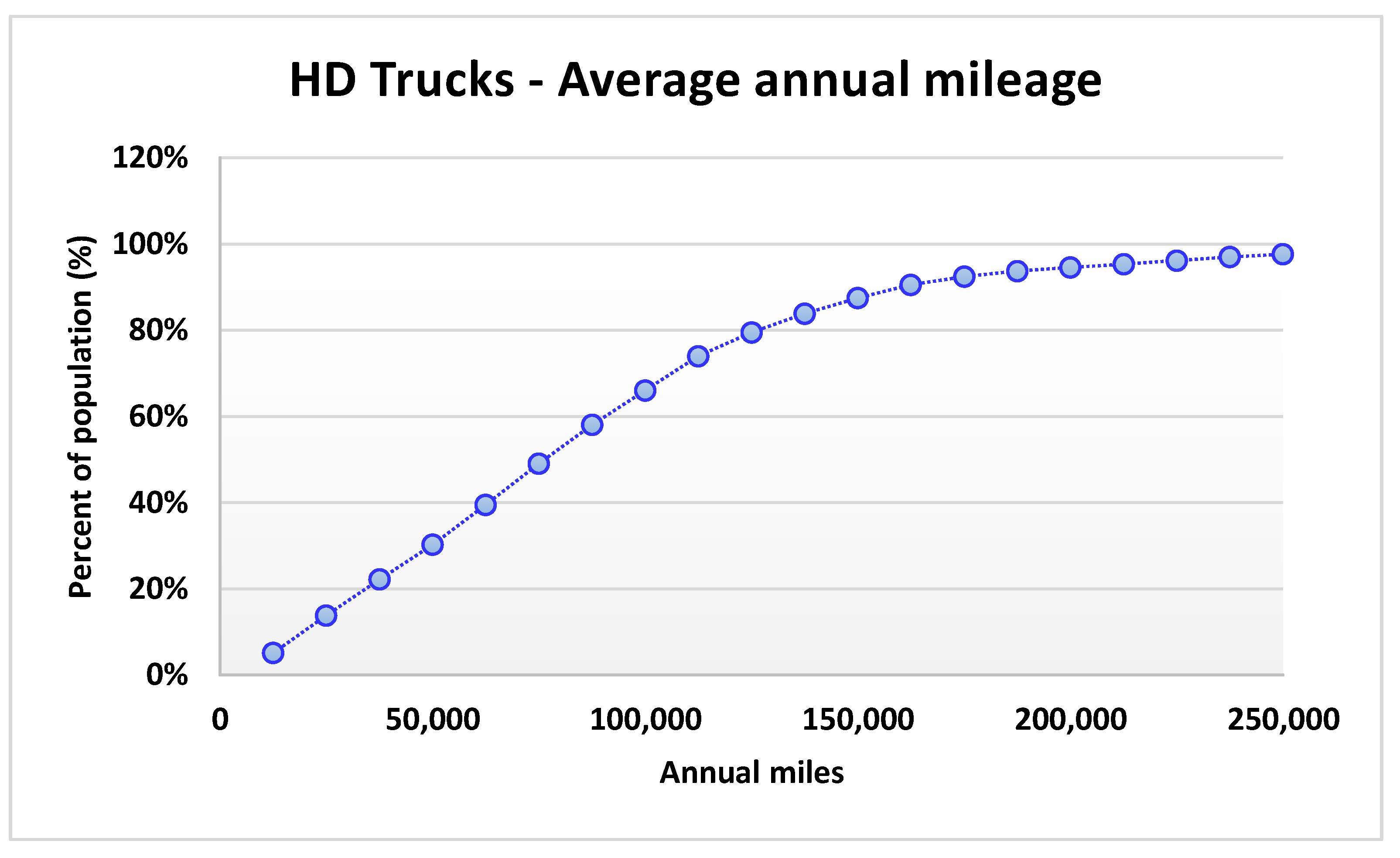
  • Class 8 population annual/daily mileage statistics;
  • Expected natural platooning due to road vehicles;
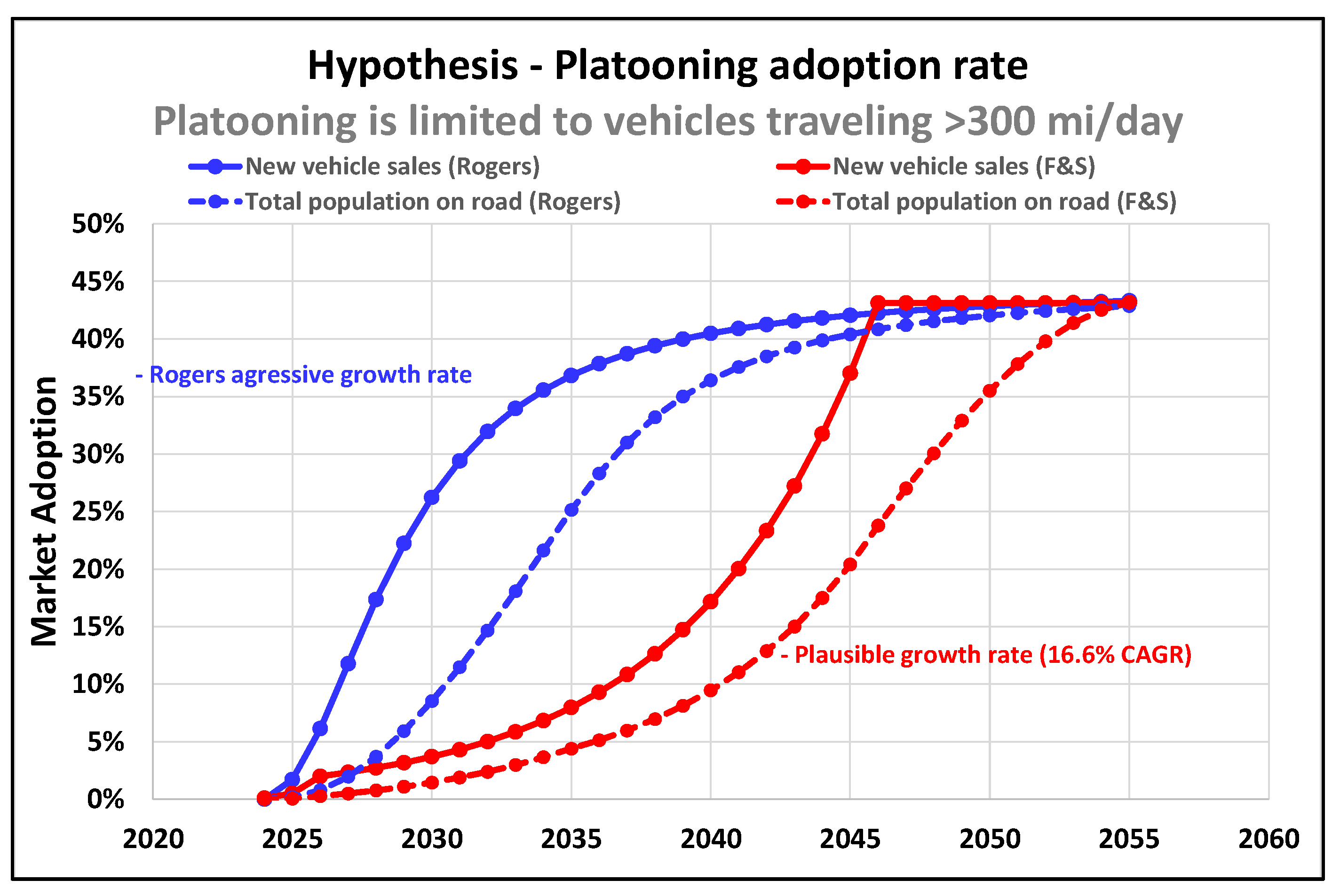
  • Technology adoption profile hypothesis.
The details of these four steps will be developed in this section.

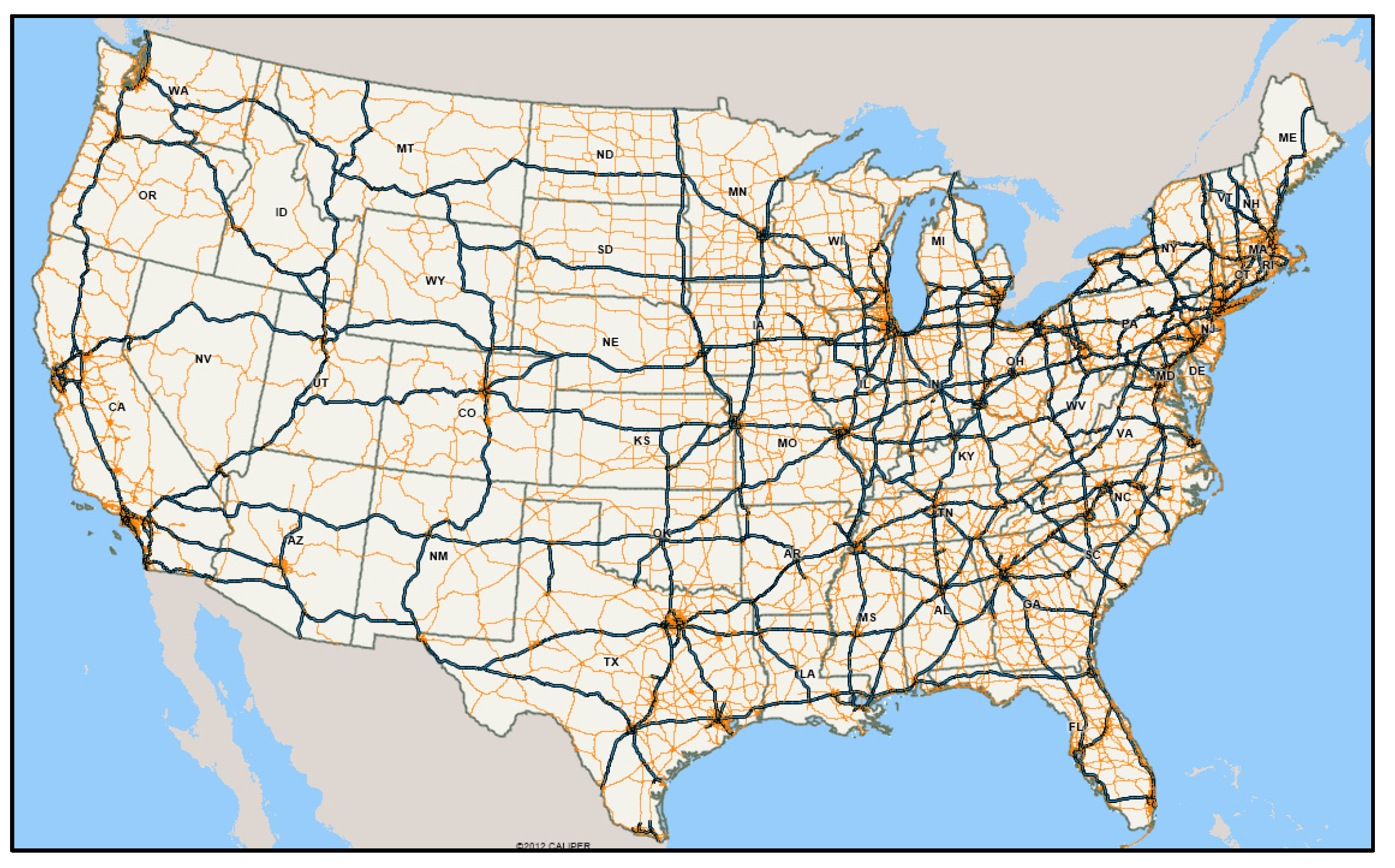
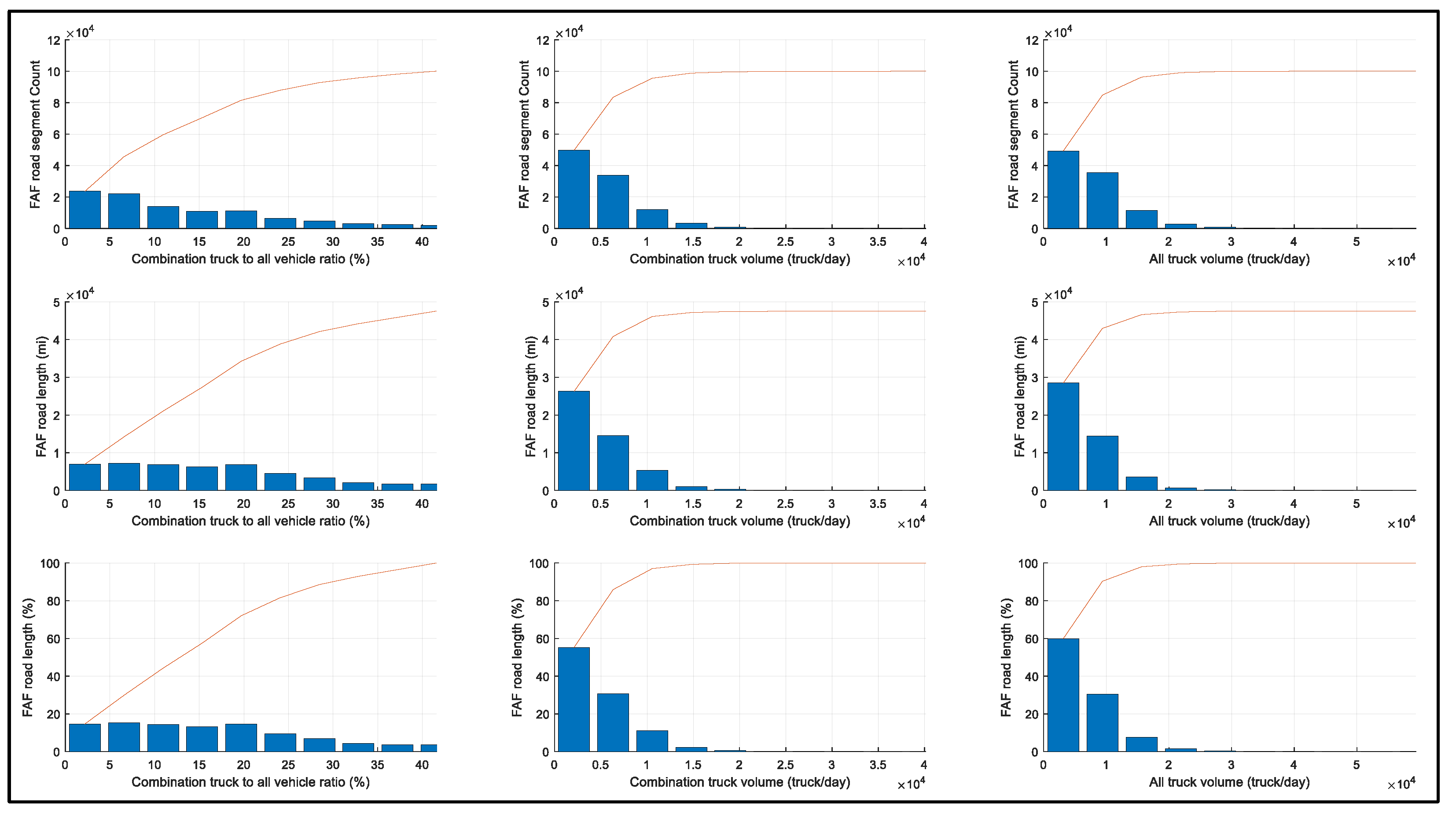
2.1. Class 8 Tractor Volume by State

Determining the tractor volume by state requires two steps. First, knowledge of the total active tractors on the US. Interstate highways needs to be identified. Second, the daily tractor volume on various segments of the US. Interstate system needs to be quantified.
The total active tractor volume has been determined through transactional examinations and routine monitoring of the vast dealership framework of the U.S. Research organizations such as ACT Research, Polk data, Vehicle In-Use Survey (VIUS), state CV registrations, and others [28]. An example of this data is shown in Figure 2, Figure 3 and Figure 4. It is important to note that only a limited number of the total number of Class 8 tractors that are registered, are in active use. In part, this is based on the reduced or special use only of older vehicles that may be in their second life use. First life vehicles that are in active use tend to see an average age in the 5.5–6 years (Figure 4). However, the average age of the total tractor population (active and inactive) ranges from 9–10 years [28]. Adoption of the new technologies such as platooning will focus on new vehicle sales and use within the active population. As such, the studies in this paper will focus on this part of the population.
In addition to the total active tractor population and annual sales in this segment, the distribution of these trucks across the US. highways is determined based on the Freight Analysis Framework (FAF) database [29]. The FAF database informs this study of the daily number of trucks traversing any given road segment. Most vehicle miles traveled by the Class 8 tractors is on interstate highways (Figure 5 and Figure 6) [30]. The FAF aggregated data for Class 8 truck volume data across the US freight corridors is shown in Figure 6. Based on both the total active tractor count and the daily truck volume on each road segment a linearly scaled quantification of tractor count by state may be established (Figure 7). In addition, states that permit platooning have also been identified [31]. The information from Figure 7, Which will be used in the techno-economic analysis of this paper, to demonstrate the sensitivity of legislation to the business case of active platooning.

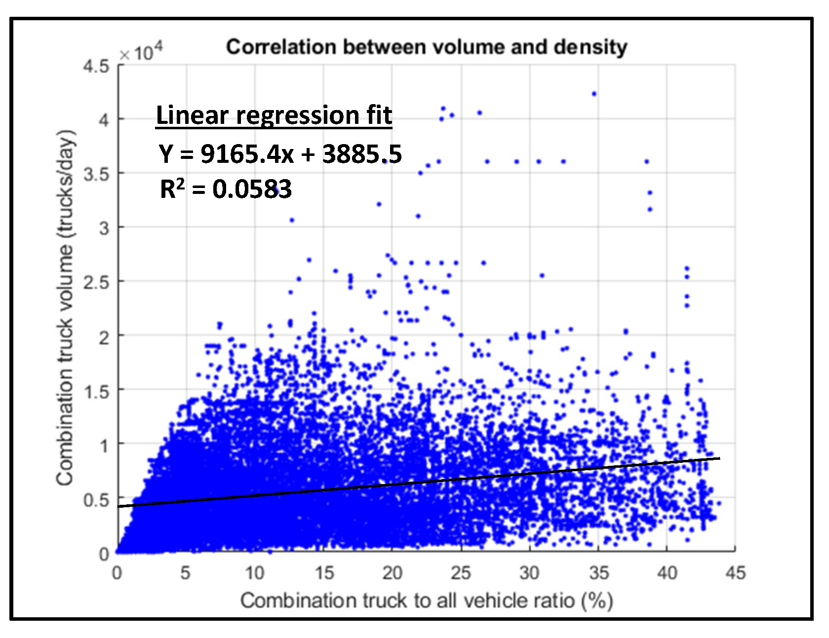
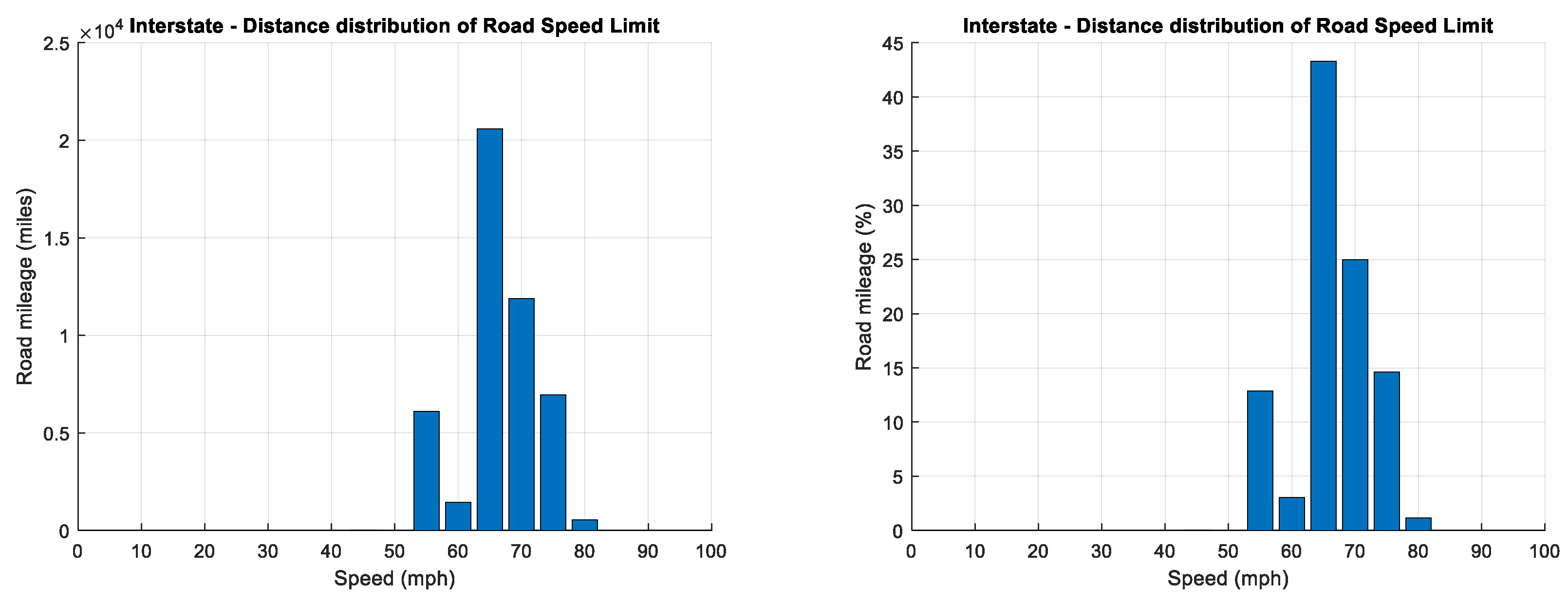
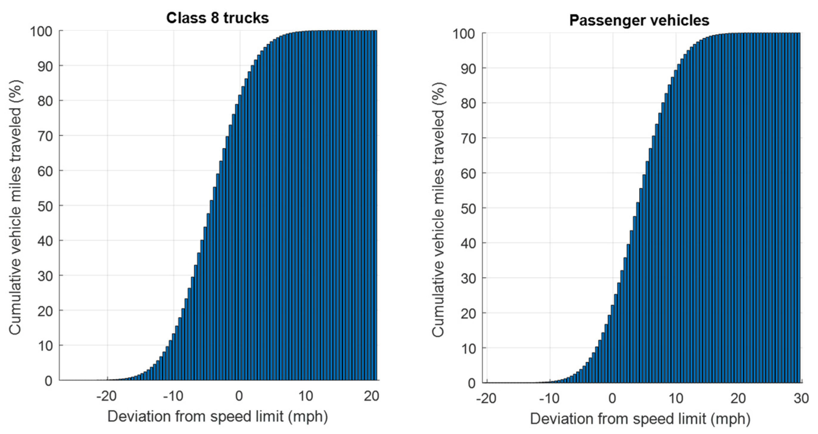
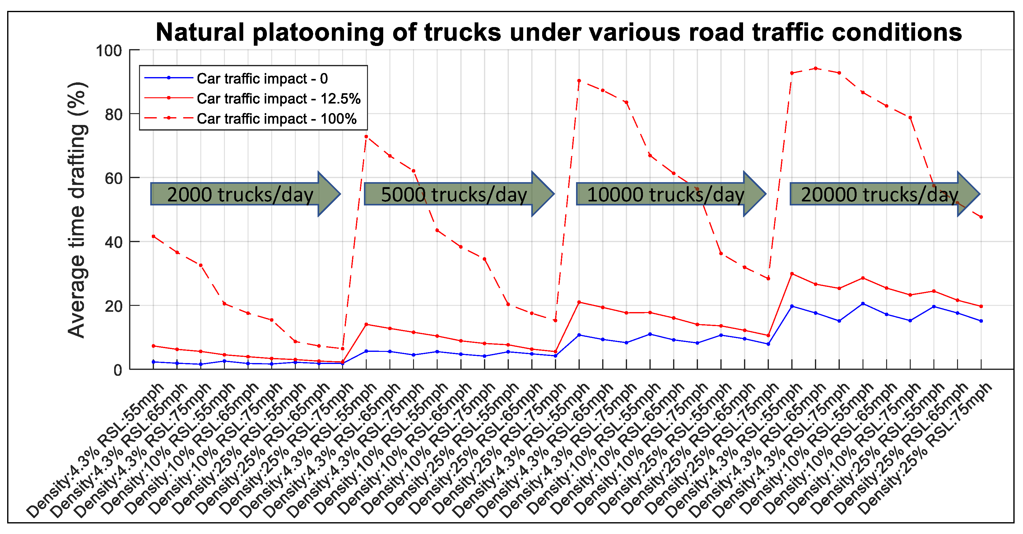
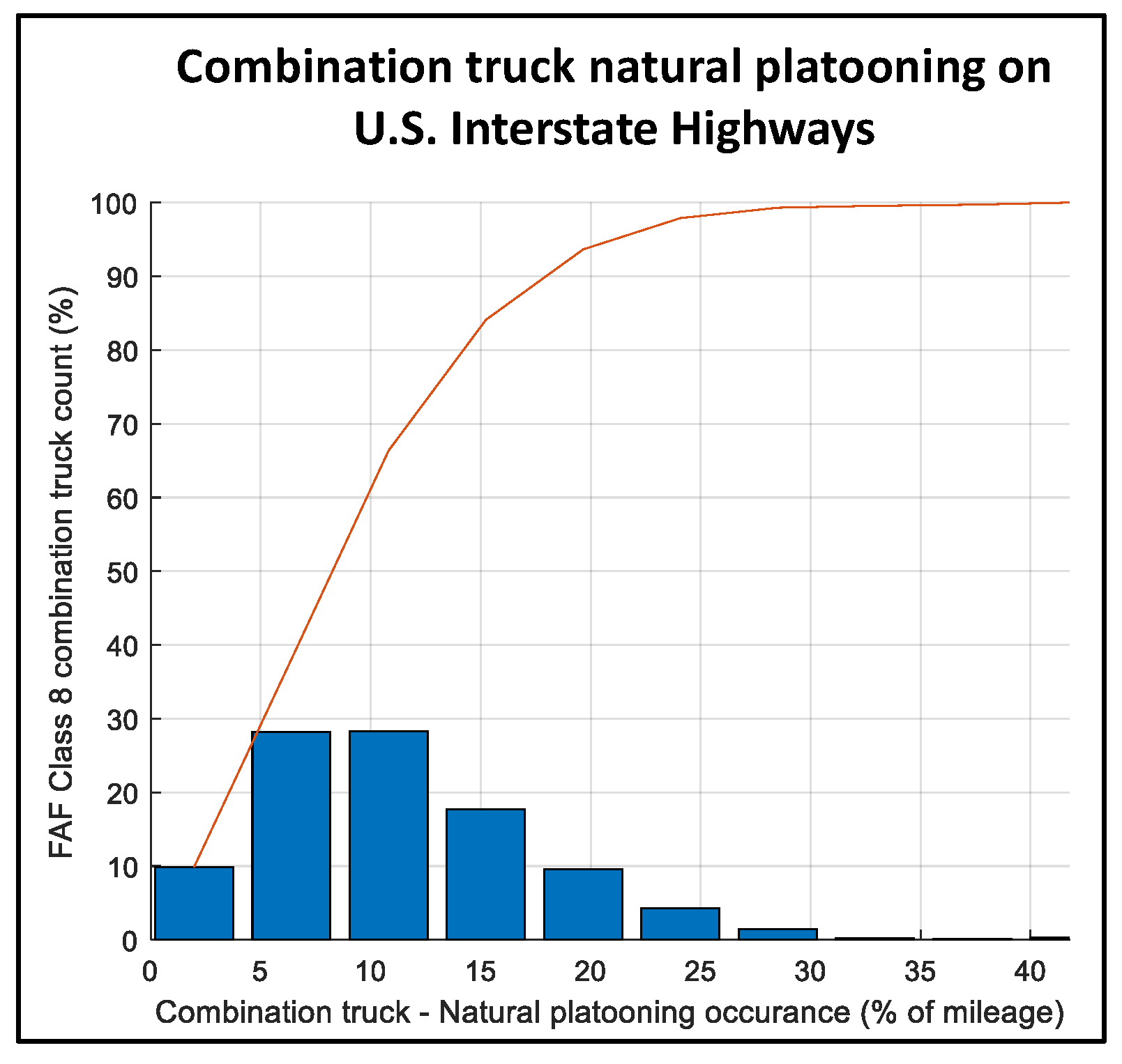
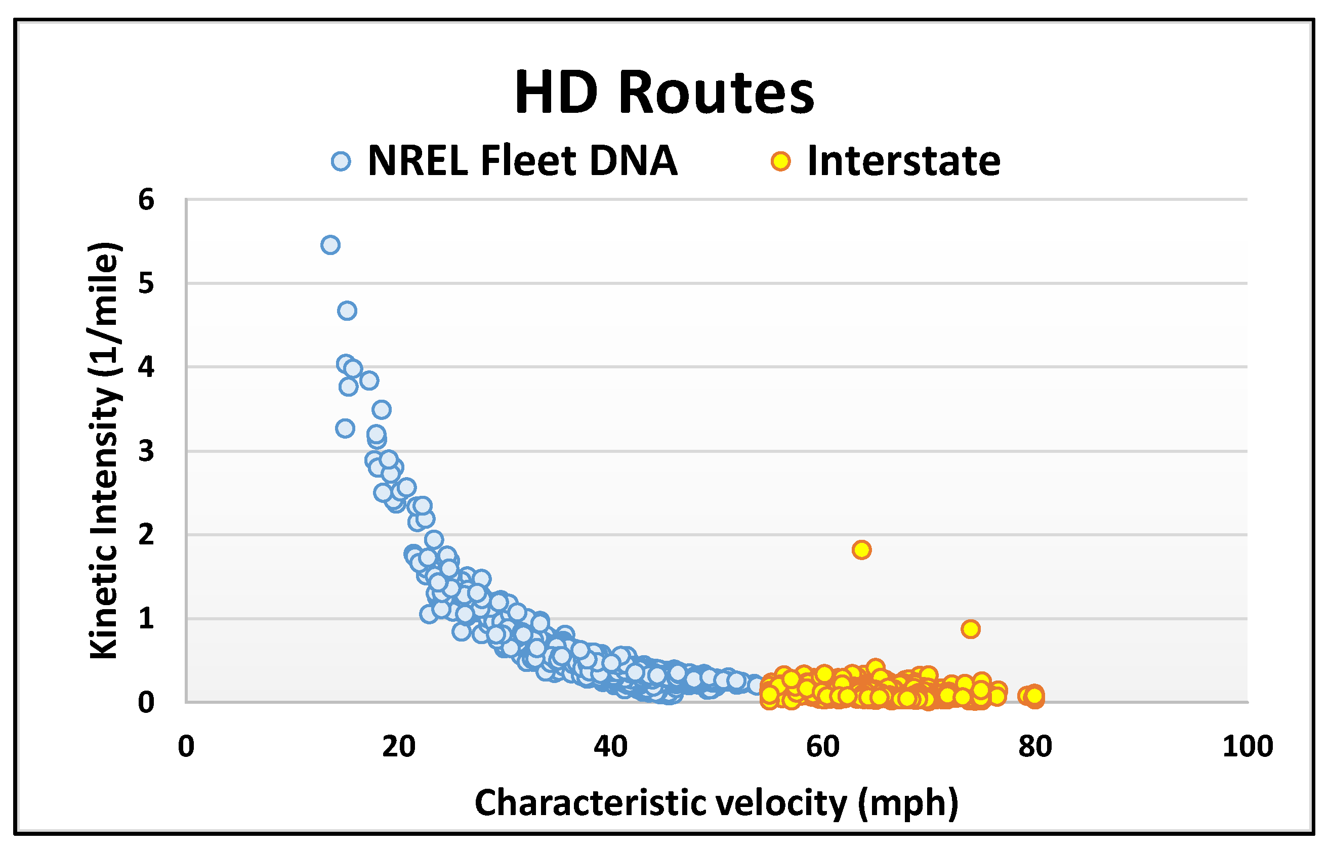
2.2. Expected Natural Platooning Due to Road-Traffic Vehicles

By reducing the aerodynamic drag losses on moving vehicles, active platooning may provide significant fuel economy improvements to 2 (or more) Class 8 tractor-trailer vehicles that are closely coupled to short following distances [9,10,12]. However, natural drafting that occurs due to traffic interactions will play a significant role in reducing the unique opportunities/benefits from platooning [9]. In other words, in the presence of other on-road traffic, reductions of vehicle aerodynamic drag (including Class 8 tractor-trailers) due to drafting will occur, which will essentially reduce the benefits of active platooning. For the purposes of this study, drafting is defined as travelling at a distance ≤ vehicle length at highway speeds. A previous study by the authors of this paper demonstrated that a substantial majority of active platooning benefits are achieved when Class 8 tractor-trailer vehicles draft within these distances [9].
Assessing the impact and frequency of natural drafting requires an assessment of the type and quantity of the surrounding vehicles on the road (from the FAF database using methodology described in Section 2.1Figure 8 and Figure 9), knowledge of the road speed limits (from the FAF database—Figure 10), and the variations of the vehicle speeds from the road speed limits (Figure 11). In Figure 8, FAF data provides information on not only the number of Class 8 tractor-trailer trucks on any given road segment but also provides a quantification of the Class 8 straight-trucks and other vehicles on the same road segment. The latter is primarily comprised of passenger vehicles and will be modeled as such going forward. This provides a measure of the tractor-trailer truck density. In Figure 9, the correlation between tractor-trailer truck count and the truck density is shown for all the interstate highways in the US. This shows a limited correlation between the two parameters, with a relatively low R-square fit, suggesting that increasing truck density does not correlate with increasing truck count.
In Figure 10, FAF data provides information on the road speed limit (RSL) of each road segment. However, it does not differentiate between truck and car road speed limits. In the absence of this information, the single-road speed limit will be used in this analysis. Additional data, if available to differentiate these two speed limits, may be readily added in. However, based on some preliminary sensitivity studies, the impact of this difference is expected to be marginal.
In Figure 11, Class 8 truck road speed limit deviation data is provided through truck observational statistics [9]. In addition, the Passenger car data is estimated from Nokia HERE traffic aggregated road speed data [33] along with the FAF truck density statistics and truck road speed limit deviation data. In this simple model, passenger car road speed limit deviation data is approximated as a linear offset from the equivalent truck observational data.
Using these results, a kinematic (no vehicle or road dynamics) simulation study is conducted to explore the impact of traffic on the likelihood that a given tractor-trailer truck will experience drafting conditions (where active platooning will not add significant fuel savings value). Critical parameters that are explored in this model include (i) the truck volume (number of Class 8 tractor-trailers/day through the highway segment), (ii) the truck density (ratio of Class 8 tractor-trailers compared to other vehicles on the highway), (iii) the road speed limit, and (iv) the drafting impact on aerodynamic drag by non-Class 8 tractor-trailer vehicles on a following vehicle (fractional equivalency to a Class 8 tractor-trailer leading vehicle). A Monte-Carlo study has been performed, where a large sample of tractor-trailers velocity profiles are modeled based on the statistics above to study the impact of these four parameters. The process of the Monte-Carlo study is as follows:
  • Define study case (Class 8 tractor-trailer volume, Class 8 tractor-trailer density, RSL, drafting impact of non-Class 8 tractor-trailer vehicles);
  • Create a sample of 1000 Class 8 tractor-trailer vehicles steady state speeds based on RSL and deviation from RSL statistics;
  • Identify the quantity of non-Class 8 tractor-trailer vehicles from the truck density;
  • Create a complementary sample of non-Class 8 tractor-trailer vehicles steady state speeds based on RSL and deviation from RSL statistics;
  • Set the initial position of each vehicle based on separation distance calculated from RSL and the total vehicle volume. For example, at RSL of 65 mph and vehicle volume of 20,000 vehicles/day (2000 Class 8 tractor-trailer trucks/day and 10% truck density) the individual separation distance is 125.53 m;
  • Simulate the position of each vehicle over n hours to determine how often each Class 8 tractor-trailer is drafting behind another vehicle;
  • Based on the drafting impact of each leading vehicle, determine the aggregated duration that each Class 8 tractor-trailer is effectively drafting.
Figure 12 show the key outputs of this study. From this, a look-up-table is created that is combined with the FAF data (from above) to establish the expected drafting impact on each Class 8 tractor-trailer on the US. Interstate highway system. The drafting impact of non-Class 8 tractor-trailer or mixed traffic vehicles is estimated as the ratio of their aerodynamic loadings, CdA, of the 2 vehicles (leading vehicle and following Class 8 tractor-trailer vehicle)—where Cd is the Coefficient of Aerodynamic Drag and A is the frontal area of the vehicles, with values obtain from [34,35,36]. From Figure 12, as expected, increasing the Class 8 truck volume also increases the natural platooning occurrences. Additionally, for a given Class 8 volume, increasing the Class 8 truck density results in fewer other vehicles on the road which reduces the natural platooning opportunities. Finally, for a given Class 8 truck volume and density, as the vehicle speeds increase (due to increasing RSL), maintaining this volume and density requires larger inter-vehicle separation distances, which reduces the natural platooning opportunities. This result is shown in Figure 13. It is observed that ~16% of the interstate miles will see > 10% natural drafting for Class 8 tractor-trailer trucks. However, from Figure 14 it is seen that ~34% of the Class 8 tractor-trailer trucks experience > 10% natural drafting while traveling on interstate roads. This suggests that the fraction of trucks that do not experience significant amounts of natural drafting on the roads, will become viable candidates for active platooning. The impact of this reduced viability will need to be considered in the techno-economics assessment going forward.

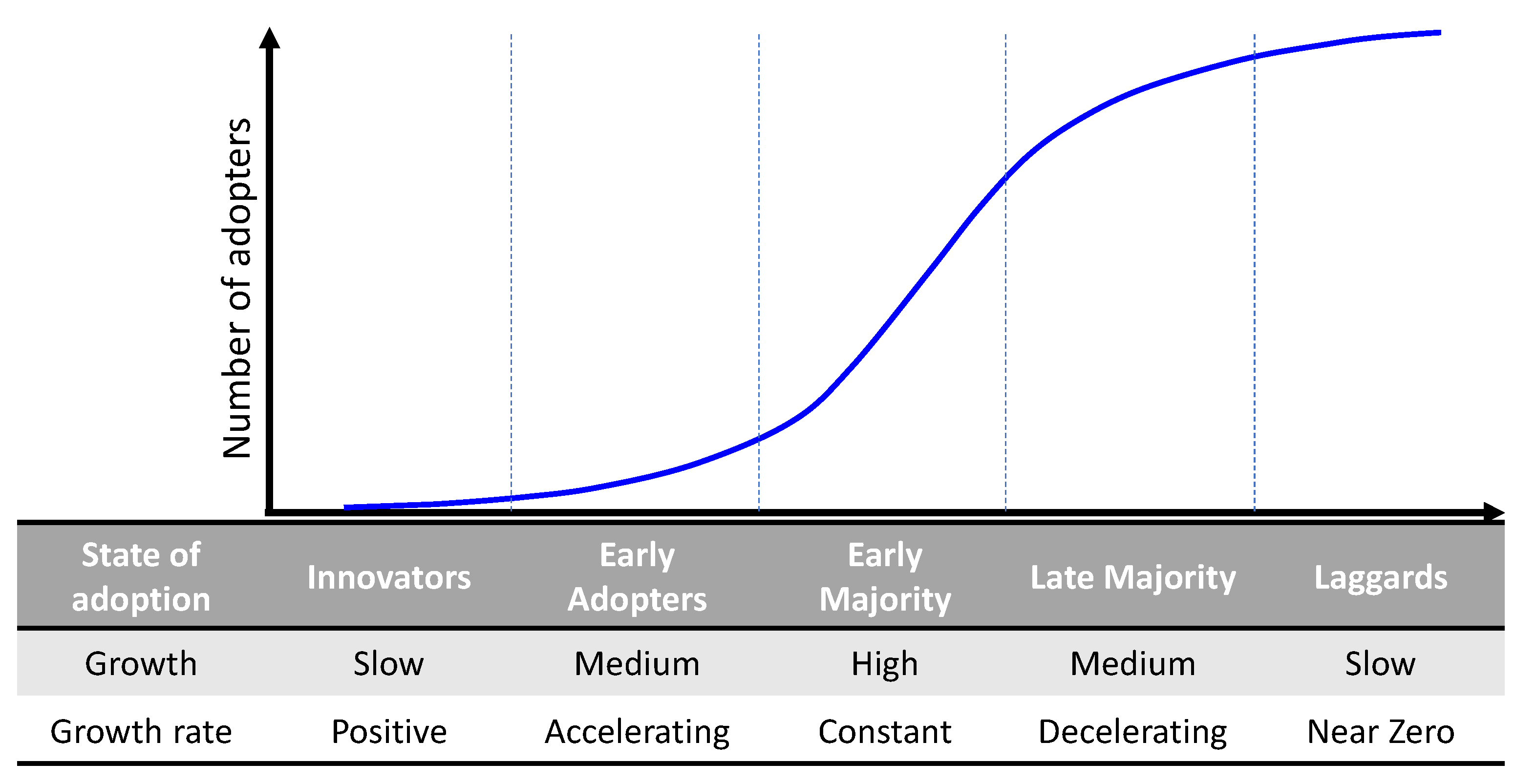
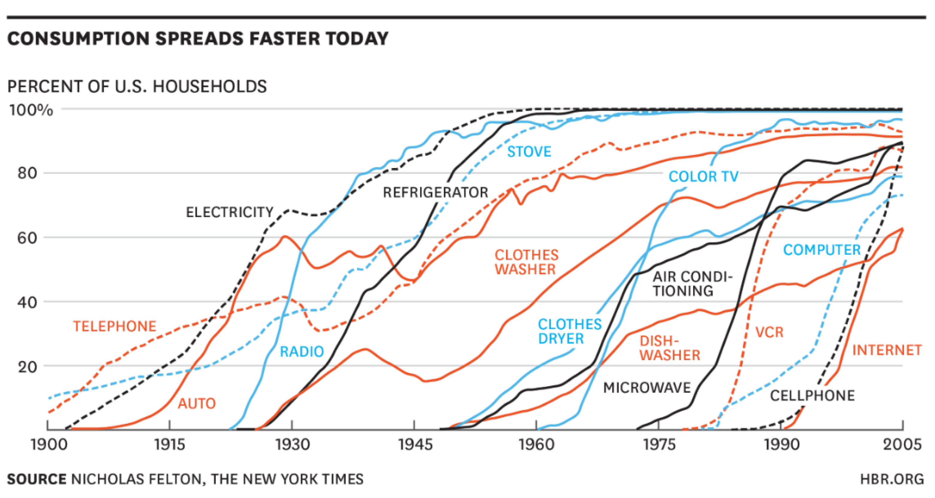
2.3. Adoption of Active Platooning by Class 8 Tractors

In addition to the above assessments on Class 8 tractor market volume, impact of natural platooning due to traffic conditions, and the annual truck mileage population characteristics, this section develops a hypothesis on active platooning technology adoption. There is great uncertainty in the adoption expectations where several possible future states may emerge. Much of this is dependent on the economics of the technology, and modeling this would be subject to the outputs of this paper. However, to establish a starting point, two hypothetical adoption models are considered. The first is based on a more generic Rogers adoption model of new technologies and would present a relatively aggressive adoption model [37]. The second is based on a Frost & Sullivan (F&S) study to create a relatively less aggressive adoption model [38].
The Diffusion of Innovation Theory, developed by Rogers, holds that disruptive technologies, products, and ideas tend to follow an ‘S’ shaped adoption curve with five stages as shown in Figure 15 (with real-world examples are shown in Figure 16). These are:
  • Adoption starts slowly, with a small group of Innovators who are willing to take a chance on a new technology before it is proven or widely accepted;
  • Next, a slightly larger group of Early Adopters accelerate the technology’s growth. This is a tipping point for the technology’s acceptance;
  • The Early Majority, convinced by the Early Adopters, result in rapid growth where the Adoption S-curve slope is the steepest;
  • Adoption continues growing as the Late Majority participate, and the technology appears almost everywhere;
  • Finally, the Laggards, accept/adopt the technology.
This may be mathematically represented as follows:
A R o g e r s = C 1 · ( y n y 0 ) 2 C 2 2 + ( y n y 0 ) 2 · C 3
where ARogers is the adoption rate at year yn, y0 is the year that adoption starts, and Ci are model coefficients (set here as C1 = 1, C2 = 5 and C3 = 43.13%).
The F&S study conducted for active platooning technology adoption states a different adoption pathway, largely based on Compound Annual Growth Rate (CAGR) for the hardware at 16.6% for North America based on several market and customer studies covering both the North America and Europe [38]. This may be mathematically represented as:
A F & S = m i n ( C 3 , y n 1 · ( 1 + R g r o w t h ) )
where AF&S is the adoption rate at year yn, Rgrowth is the CAGR (set here as 16.6%), and C3 is a model coefficient (set here as 43.13%). This model also assumes a small non-zero value for the first year of adoption (set here at 0.5%).
Their study asserts that government support will represent a significant factor in the uptake of autonomous trucks by the year 2025. This is hinged on the expectation that every new truck produced will be mandated to have advanced safety systems (sensors, cameras, electronic controls, and stability) installed, thus providing an enabling platform for platooning and other autonomous driving technologies. However, both models are agnostic to specific policies related to platooning and are largely customer technology adoption curves. Policy factors will act as critical drivers or activation points. Given the uncertainty associated with this, the impact of policy in the adoption curves will be deferred for future research.
For this paper, the Rogers and the F&S models provide two limiting adoption models of active platooning technology in new vehicles sold. Additional sensitivity will be explored in the results of the next sections. Further, an upper limit must be identified to the adoption rate models. In this study, the upper bound is specified based on the Class 8 tractor population that cover more than 300 miles per day, suggestive of regional and line haul applications, where there may be substantial opportunity for active platooning. From Figure 17 this is estimated at 43.13% of the population (using annual Vehicle Miles Traveled). This may be adjusted if additional application usage information is available. Moreover 2, from the average life (~6 years) of the active Class 8 tractor population is used to determine the total population penetration of the active platooning technology. In other words, based on the penetration of active platooning technology for new Class 8 tractors sold and the average life of the tractor before it is removed from service, the total penetration of the active platooning technology in all active Class 8 tractors may be determined. These results are shown in Figure 18.

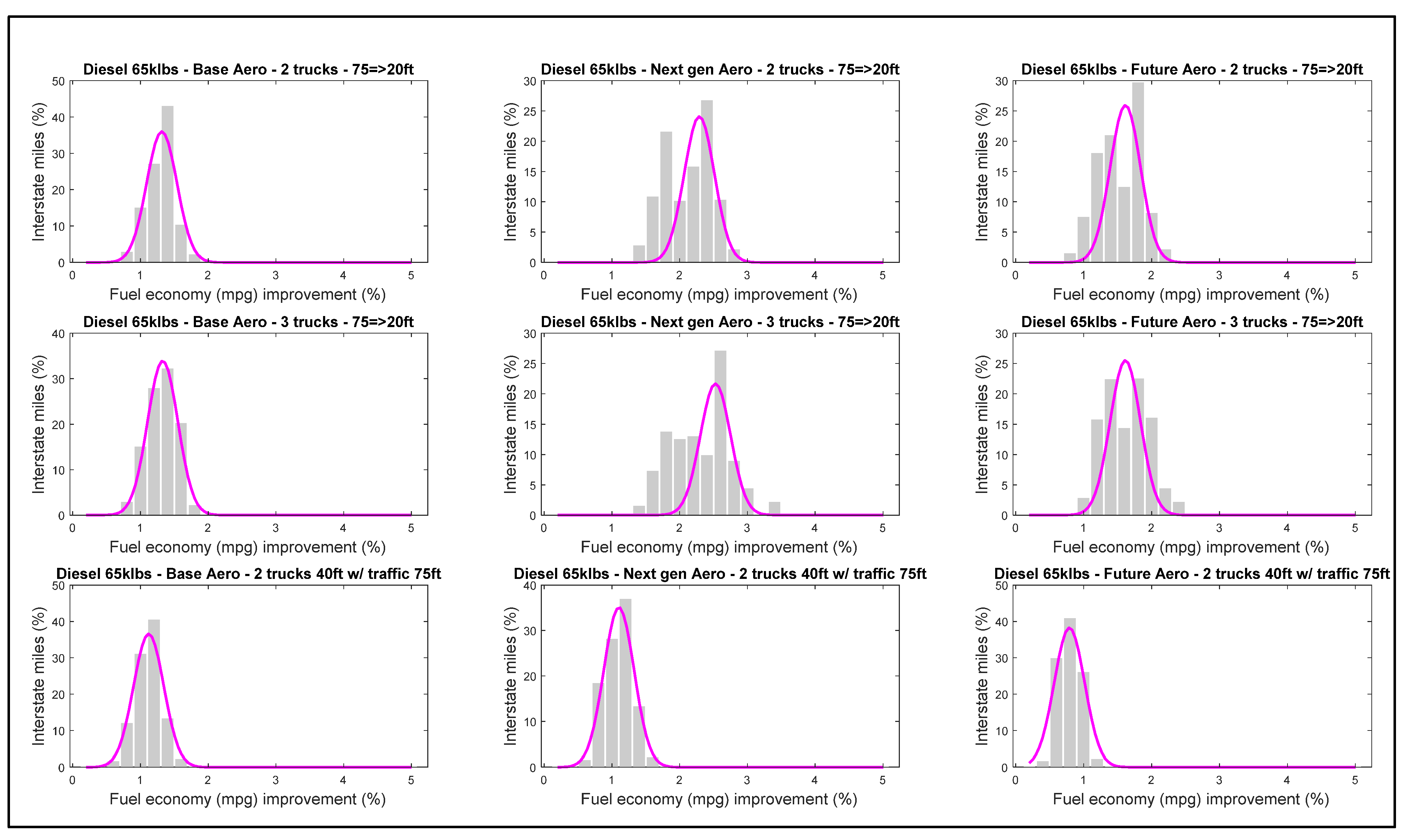
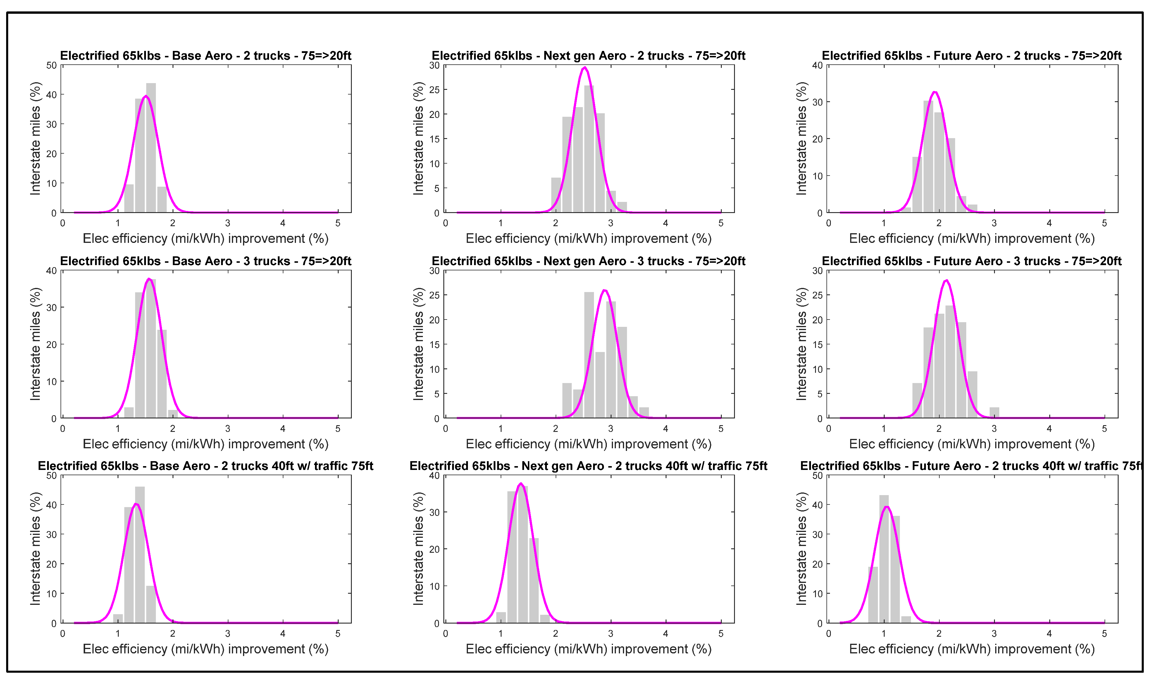
3. Interstate Road Models and Active Platooning Energy Improvements

For this analysis all Interstate Road elevation (grade) and speed limits are extracted from the Nokia HERE database using FAF (Freight Analysis Framework) interstate route coordinates (Figure 5) [29]. Alternatively, the US Census Bureau provides shapefiles for primary roads that may be used but are considered less accurate [42]. Approximately 47 k miles of road data has been extracted and grouped into route segments ranging from ~30–60 miles. All route segments are bidirectional to eliminate the effects of any net elevation change. These are compared against a broader range of Class 8 HD truck duty cycles (Figure 19) [9,10,41]. This broader range of duty cycles are polled from real-world Class 8 HD truck logged cycles and represent drayage, short haul, regional haul and line haul applications. These duty cycles are characterized based on their Kinetic Intensity and Characteristic Velocity (where Kinetic Intensity is a ratio of characteristic acceleration to characteristic velocity; characteristic acceleration measures the inertial work to accelerate and/or raise the vehicle per unit mass per unit distance over the cycle; characteristic velocity measures the ratio of the average cubic speed to the average speed) described in mathematical detail in [41].
Figure 20 and Figure 21 shows the fuel economy of a single Class 8 tractor-trailer weighing 65 klbs with the Next Gen aerodynamics package (defined in the introduction), using a conventional diesel and electrified powertrain, respectively, derived through vehicle simulation studies [9,10]. The greater spread seen in Figure 21 in comparison to Figure 20 is based on the regenerative potential of the route due to grade and speed.
Figure 22 (conventional diesel powertrain) and Figure 23 (electrified powertrain) show that the active platooning fuel economy benefits of operating 2, 3 and 5 truck platoons with varying separation distances (20, 40 and 75 ft) and different aerodynamic features (described in the introduction) across all of the interstate routes [9]. Both evaluations show the average platoon FE gains compared against a single vehicle. In general, the results suggest that reducing the separation distance and increasing the number of vehicles in the platoon increases the FE gains. It is notable that the average platooning energy efficiency of an electrified powertrain is ~1.77% (~1.83% at 65 klbs; ~1.72% at 80 klbs) at 20 ft and ~1.67% (~1.79% at 65 klbs; ~1.55% at 80 klbs) at 40 ft better than a diesel powertrain (ignoring the influence of road traffic) [9]. Several other parameters may also be considered in characterizing these behaviors (including lateral variations, wind yaw, ambient temperature, ambient pressure, cooling system flow, etc.) but were outside the scope of these previous studies.
Figure 24 (conventional diesel powertrain) and Figure 25 (electrified powertrain) describe simple scenarios of following another Class 8 truck i.e., impact of traffic [9]. The results explore the impact of (i) drafting in traffic at 75 ft versus platooning at 20 ft with 2 similar HD vehicles; (ii) drafting in traffic at 75 ft versus platooning at 20 ft with three similar HD vehicles; (iii) drafting in traffic at 75 ft in both a single vehicle and a 2-truck (40 ft) platoon. Under these conditions active platooning FE benefits significantly drop [9]. This indicates that drafting or natural platooning within a vehicle body length will mitigate the benefits of active platooning (as previously discussed). The results of this study will be used to establish variations of active platooning energy efficiency improvements for the techno-economic models.

4. Value Proposition of L1–L1 Automation

The assessment of the economic measures of active platooning explores several critical factors. These factors include: (i) powertrain type—diesel and electric, (ii) adoption model—Frost & Sullivan and Rogers, (iii) potential price of added technology—$500 → $2500, (iv) probability of finding an active platooning partner—5% → 50%, (v) state legislative constraints—20 states → all states, and (vi) scenarios for optimistic (best) case/base case/pessimistic (worst) case for platooning (Table 1 and Table 2).
The economic measures include end-user payback time (if technology is bought out complete) and a supplier revenue model (set at 20% of the savings potential based on a technology lease model of pay-per-use [38]). Note that in the 3 scenarios created (Table 1 and Table 2), the values for the various factors are based on known active Class 8 tractor usage [28,43], replacement cycles discussed in Section 2, single vehicle and platooning vehicle energy consumption discussed in Section 3, fuel energy cost based on EIA databases [44], and platoon-able miles based on observed highway variations. It is worth noting here that the fraction of platoonable miles is obtained from examining the real-world drive cycles (Figure 19) and identifying the duration that the vehicle operates at highway speeds for periods greater than 30 min. These are averaged for all of the drive cycles bounded by the vehicle daily mileage range specified in Table 1 and Table 2 and rounded to the nearest 5%. In the worst-case scenario, the combination of parameter values is selected from one end of the feasible range such that FE savings from platooning will be less promising. Likewise in the best-case scenario, the combination of parameter values is selected at the other end of the feasible range and will be more favorable for platooning. Finally, the base-case is established by taking median values for these parameters.

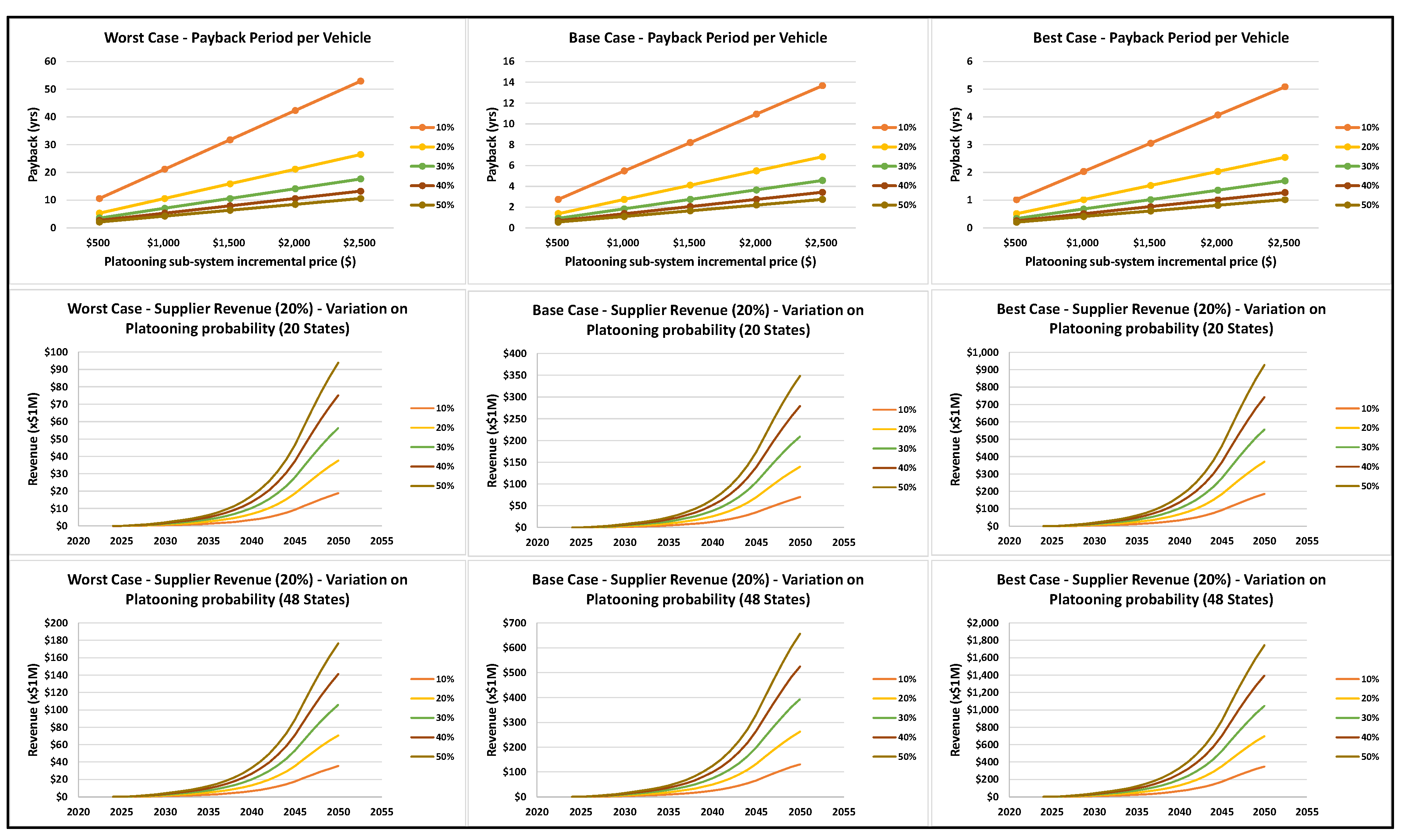
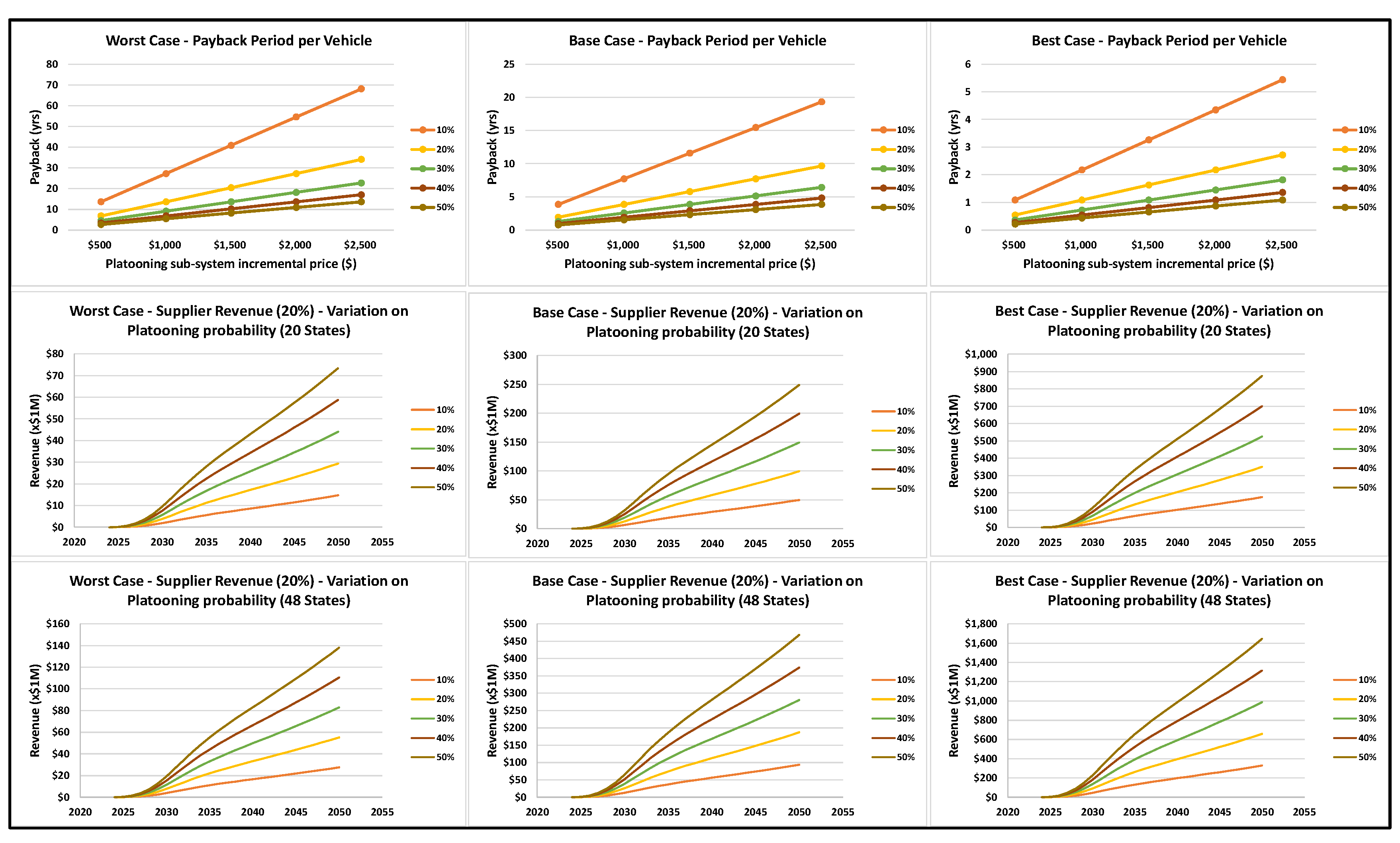
4.1. Scenario 1—Diesel v. BEV

In this scenario, the payback and revenue potential of an active platoon of 2 Class 8 tractor-trailers with diesel and electric powertrains (using the F&S adoption model) is assessed. Figure 26 and Figure 27 show the results for this. Here, the implications of the potential price of the added technology ($500 to $2500), the probability of finding an active platooning partner (5% to 50%), the state regulation limits, and the worst-case to best-case are shown. Note that the L1 platooning capability will require added controls, wiring harness, electronic interface to the engine/brakes (via Controller Area Network), radar, and telematics. New vehicles are likely to be equipped with telematics and Adaptive Cruise Control. This allows the platooning system to leverage the common telematics and radar hardware. As such, and additional equipment prices are expected to fall within the range specified. The main takeaways from this are the following:
  • Diesel payback: In the worst-case scenario, payback exceeds 2.1 years for all of the conditions shown and may not meet NA market expectations (payback periods of ≤ 1.5 years). However, by extrapolating the results, a payback of ≤ 1.5 years occurs if either
    Technology price is $500 and probability of finding a platooning partner > 63.1%
    Technology price is $2500 and probability of finding a platooning partner > 88.6%;
  • Diesel payback: In the best-case scenario payback of ≤ 1.5 years occurs if either
    Technology price is $500 and probability of finding a platooning partner > 7.6%
    Technology price is $2500 and probability of finding a platooning partner > 34%;
  • Diesel revenue: In the worst-case scenario, limited by current regulations (20 states), the revenue potential at:
    10 years of adoption will range from $0.5 M to $5.1 M
    20 years of adoption will range from $3.8 M to $38.3 M;
  • Diesel revenue: In the best-case scenario, unlimited by current regulations (48 states), the revenue potential at:
    10 years of adoption will range from $10 M to $99.8 M
    20 years of adoption will range from $72.2 M to $722.1 M;
  • Electric payback: In the worst-case scenario, payback exceeds 2.1 years for all of the conditions shown and may not meet NA market expectations (payback periods of ≤1.5 years). However, by extrapolating the results, a payback of ≤ 1.5 years occurs if either
    Technology price is $500 and probability of finding a platooning partner > 70.2%
    Technology price is $2500 and probability of finding a platooning partner > 90.5%;
  • Electric payback: In the best-case scenario, payback of ≤ 1.5 years occurs if either
    Technology price is $500 and probability of finding a platooning partner > 8.1%
    Technology price is $2500 and probability of finding a platooning partner > 36.4%;
  • Electric revenue: In the worst-case scenario, limited by current regulations (20 states), the revenue potential at:
    10 years of adoption will range from $0.4 M to $4 M
    20 years of adoption will range from $3 M to $29.7 M;
  • Electric revenue: In the best-case scenario, unlimited by current regulations (48 states), the revenue potential at:
    10 years of adoption will range from $9.3 M to $93.3 M
    20 years of adoption will range from $67.5 M to $675.2 M.

4.2. Scenario 2—Diesel v. BEV—Changed Adoption Model

In this scenario, the payback and revenue potential of an active platoon of 2 Class 8 tractor-trailers with diesel and electric powertrains (using the Rogers adoption model) is assessed. Figure 28 and Figure 29 show the results for this. Here, the implications of the potential price of the added technology ($500 to $2500), the probability of finding an active platooning partner (5% to 50%), the state regulation limits, and the worst-case to best-case are shown. The main takeaways from this are the following:
  • Diesel payback: Adoption model change does not have any impact to the payback, and these are as previously reported;
  • Diesel revenue: In the worst-case scenario, limited by current regulations (20 states), the revenue potential at:
    10 years of adoption will range from $3.2 M to $31.7 M
    20 years of adoption will range from $7 M to $70.2 M;
  • Diesel revenue: In the best-case scenario, unlimited by current regulations (48 states), the revenue potential at:
    10 years of adoption will range from $61.9 M to $619 M
    20 years of adoption will range from $132.3 M to $1323.1 M;
  • Electric payback: Adoption model change does not have any impact to the payback, and these are as previously reported;
  • Electric revenue: In the worst-case scenario, limited by current regulations (20 states), the revenue potential at:
    10 years of adoption will range from $2.5 M to $24.6 M
    20 years of adoption will range from $5.4 M to $54.5 M;
  • Electric revenue: In the best-case scenario, unlimited by current regulations (48 states), the revenue potential at:
    10 years of adoption will range from $57.9 M to $578.8 M
    20 years of adoption will range from $123.7 M to $1237.2 M.

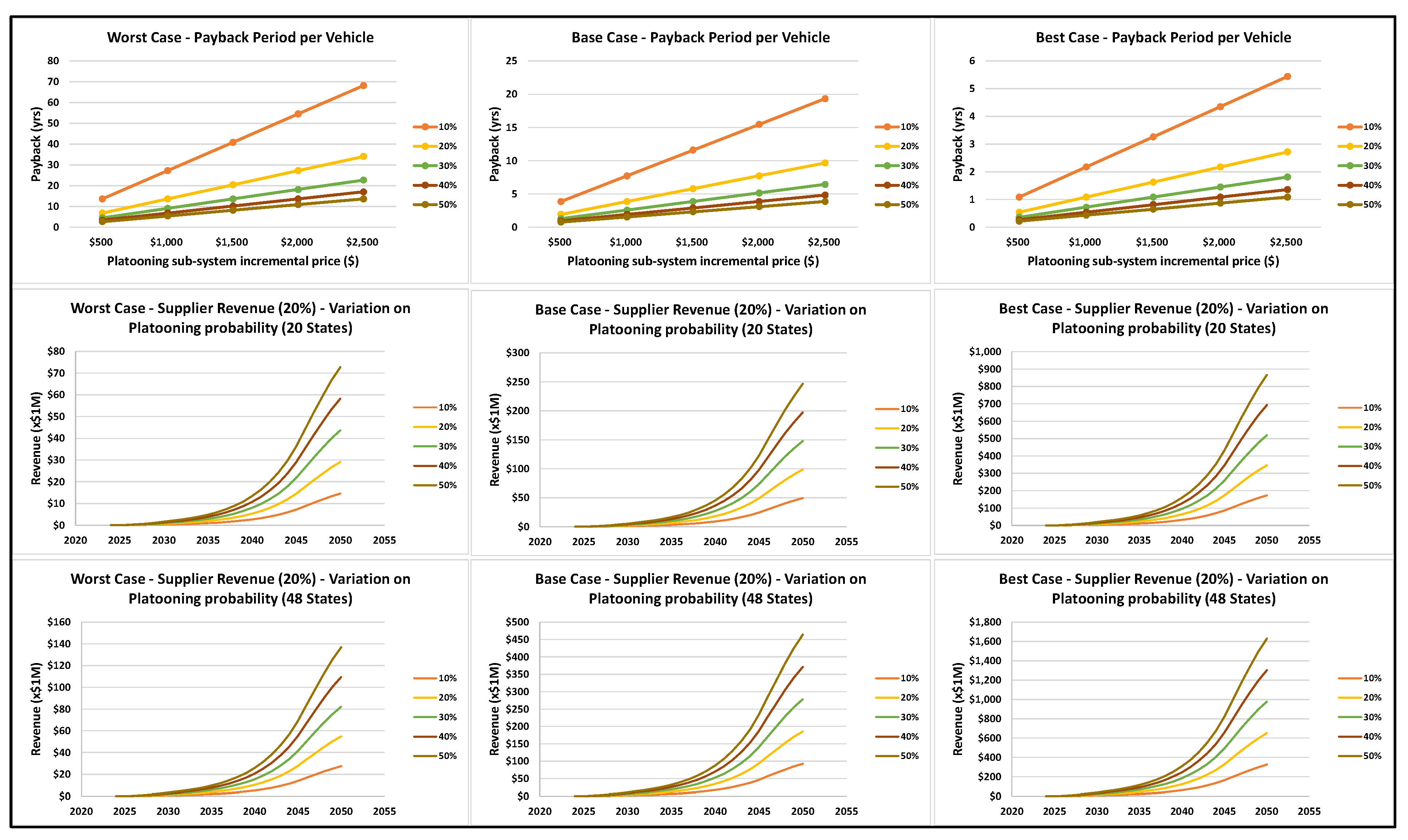
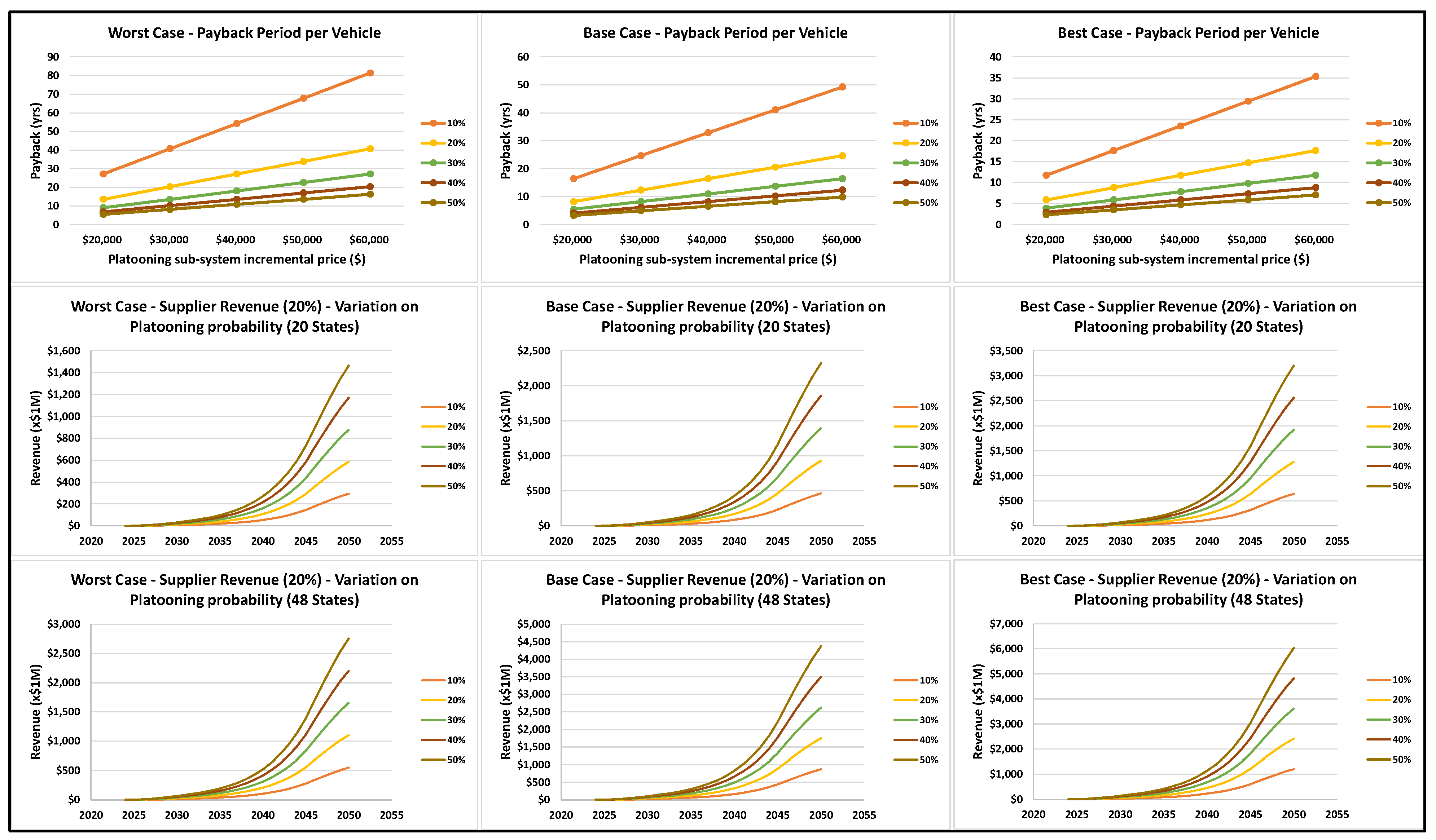
5. Value Proposition of L1–L4 Automation (Following Vehicle)

A key factor introduced to the analysis in this section is the added value of L4 platooning of all of the following vehicles. With L4 platooning, additional value is generated by asserting that the operator of a following vehicle in the platoon, will be able to rest during the mission [45]. This rest period will count towards the operator off-time. This rest period will ideally translate to added driving time for the vehicle through an effective increase in operator HoS [45]. There is uncertainty that regulatory agencies will follow through with this concept. However, in the event of this possibility this section will examine the sensitivity of this increase to HoS. Note that for a 2-truck L1–L4 platoon, the effective increase in HoS for the following vehicle/operator will apply across both vehicles to assess the net benefits (missions will see increased operating time by reversing the order of the vehicles).
The value of the operational time for vehicles has been evaluated for more than 40 years since it was noted to be an important part of economic analysis in transport planning [46]. Several efforts have gone into assessing this metric since then. While we do not intend to provide a comprehensive assessment of these studies, several notable ones are highlighted. ATRI provides periodic reports for more accurate trucking industry operational cost data by motor carriers and government transportation planners [43]. Haning et al. published one of the first reports estimating the value of time for CVs [47]. They evaluated time savings through the “net operating profit” approach and calculated a value of time range between $30.16/h and $39.17/h. Using Interstate Commerce Commission (ICC) freight data, Adkins et al. derived the CV value of time for each ICC region based on the cost-saving method [48]. For the Pacific region, the value of time for intercity trucks was estimated at $46.28/h. Waters et al., compiled a summary of CV values of time used by fourteen agencies in various countries (six in the United States, three in Canada, three in Australia, one in New Zealand, and one in Norway/Sweden) for evaluating costs-benefits of highway projects [49]. The values of time ranged from $25.13/h to $61.7/h for agencies in the United States and Canada. Kawamara studied the impact of various fleet configurations to determine a median, mean and the standard deviation for the value of CV time [50]. These were estimated by the random coefficient logit model for the entire sample as $24.09, $40.56/h and $55.46/h, respectively. Smalkoski et al., used six scenarios of Adaptive Stated Preference (ASP) to estimate the value of time for CV operators in Minnesota [51]. Value of time for trucks was estimated from stated preference data collected in California. Truckers were asked about a choice between an existing free road versus a toll facility for different combinations of travel time and cost. Estimation was based on the point of diversion at which the switch of facility occurred in the stated preference questions and on the use of a modified logit model in which the coefficients to be estimated were assumed to be distributed lognormally across the population. The model provided an estimate for the average CV value of time in Minnesota of $69.41/h. The values of each study have been updated to reflect 2021 prices based on an average annual inflation [52].
Here, the assessment of the economic measures of active platooning explores the following critical factors: (i) powertrain type—diesel and electric, (ii) adoption model—Frost & Sullivan and Rogers, (iii) potential price of added technology per vehicle—$20,000 to $60,000 (for L4 capabilities on both vehicles to support interchangeable vehicle ordering), (iv) probability of finding an active platooning partner—5% to 50%, (v) state legislative constraints—20 states to all states, (vi) additional value of each hour of vehicle operation—$24.09/h to $40.56/h [53], and (vii) scenarios for optimistic (best) case/base case/pessimistic (worst) case for platooning (Table 1 and Table 2). While the specific L4 architecture, capabilities and pricing is outside the scope of this research, depending on the operating design domain expectations, the additional hardware may include a full L4 sensing and controls suite including electrical power capabilities to support this system. The hardware devices for a L4 autonomous vehicle generally include: 6–12 cameras, 3–12 radars, 1–3 LiDARs, 2 Global Navigation Satellite Systems/Inertial Measurement Units and 2 computing platforms (including the redundant one). Due to OEM integration dilution, higher volume component cost reductions, and subscription fees, it is difficult to identify specific price increases for this system, as such this study has incorporated a meaningful expected lifecycle price range.
As before, the economic measures include end-user payback time (if technology is bought out complete) and a supplier revenue model (while difficult to predict the revenue model, in this study it is set at 20% of the savings potential based on a technology lease model of pay-per-use, with the operational gains also being included [38]).

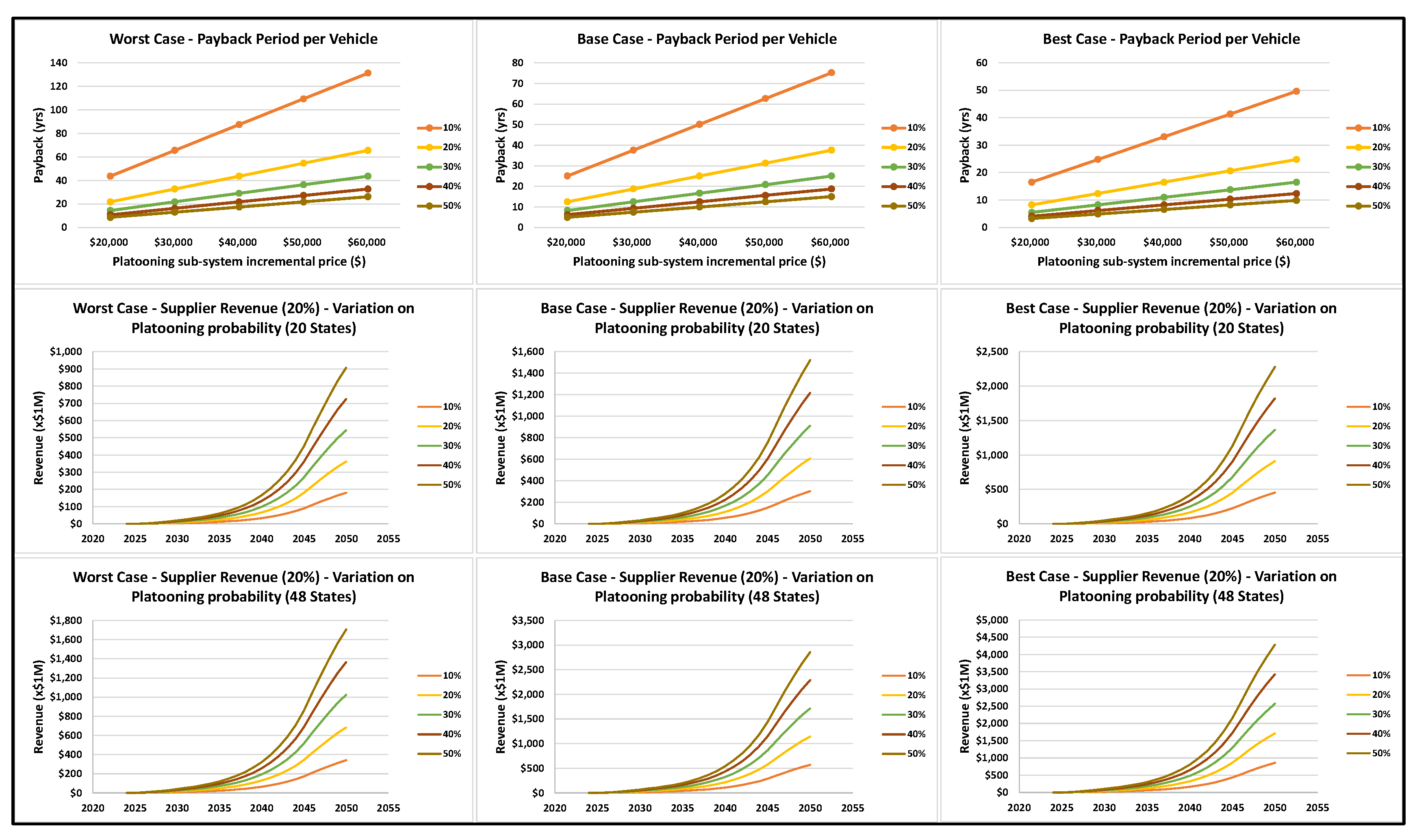
5.1. Scenario 1—Diesel v. BEV—Driver/Vehicle Hourly Value at Median ($24.09/h)

In this scenario, the payback and revenue potential of an active platoon of 2 Class 8 tractor-trailers with diesel and electric powertrains (using the F&S adoption model) is assessed. Figure 30 and Figure 31 show the results for this. Here the implications of the potential price of the added technology ($20,000 to $60,000), the probability of finding an active platooning partner (5% to 50%), the state regulation limits, the value of each additional hour of service is $24.09/h, the L4 operator resting equivalency factor is 0.25 (for each of hour of L4 rest, the operator gains 15 min of additional drive time) and the worst-case to best-case are shown. The main takeaways from this are the following:
  • Diesel payback: In the worst-case scenario, payback of ≤ 1.5 years occurs if either
    Technology price is $20,000 and probability of finding a platooning partner > 87.3%
    Technology price is $60,000 and probability of finding a platooning partner > 92.4%;
  • Diesel payback: In the best-case scenario, payback of ≤ 1.5 years occurs if either
    Technology price is $20,000 and probability of finding a platooning partner > 74.6%
    Technology price is $60,000 and probability of finding a platooning partner > 88.2%;
  • Diesel revenue: In the worst-case scenario, limited by current regulations (20 states), the revenue potential at:
    10 years of adoption will range from $4.9 M to $49.4 M
    20 years of adoption will range from $37 M to $370.3 M;
  • Diesel revenue: In the best-case scenario, unlimited by current regulations (48 states) the revenue potential at:
    10 years of adoption will range from $24.5 M to $245.3 M
    20 years of adoption will range from $177.5 M to $1775.5 M;
  • Electric payback: In the worst-case scenario, payback of ≤1.5 years occurs if either
    Technology price is $20,000 and probability of finding a platooning partner >87.5%
    Technology price is $60,000 and probability of finding a platooning partner >92.5%;
  • Electric payback: In the best-case scenario, payback of ≤ 1.5 years occurs if either
    Technology price is $20,000 and probability of finding a platooning partner > 75.1%
    Technology price is $60,000 and probability of finding a platooning partner > 88.4%;
  • Electric revenue: In the worst-case scenario, limited by current regulations (20 states) the revenue potential at:
    10 years of adoption will range from $4.8 M to $48.3 M
    20 years of adoption will range from $36.2 M to $361.8 M;
  • Electric revenue: In the best-case scenario unlimited by current regulations (48 states) the revenue potential at:
    10 years of adoption will range from $23.9 M to $238.8 M
    20 years of adoption will range from $172.9 M to $1728.6 M.

5.2. Scenario 2—Diesel v. BEV—Changed Adoption Model

In this scenario, the payback and revenue potential of an active platoon of 2 Class 8 tractor-trailers with diesel and electric powertrains (using the Rogers adoption model) is assessed. Figure 32 and Figure 33 show the results for this. Here, the implications of the potential price of the added technology ($20,000 to $60,000), the probability of finding an active platooning partner (5% to 50%), the state regulation limits, the value of each additional hour of service is $24.09/h, the L4 operator resting equivalency factor is 0.25 (for each of hour of L4 rest, the operator gains 15 min of additional drive time) and the worst-case to best-case are shown. The main takeaways from this are the following:
  • Diesel payback: Adoption model change does not have any impact to the payback and these are as previously reported;
  • Diesel revenue: In the worst-case scenario, limited by current regulations (20 states) the revenue potential at:
    10 years of adoption will range from $30.7 M to $306.6 M
    20 years of adoption will range from $67.9 M to $678.6 M;
  • Diesel revenue: In the best-case scenario, unlimited by current regulations (48 states) the revenue potential at:
    10 years of adoption will range from $152.2 M to $1521.9 M
    20 years of adoption will range from $325.3 M to $3253.4 M;
  • Electric payback: Adoption model change does not have any impact to the payback and these are as previously reported
  • Electric revenue: In the worst-case scenario, limited by current regulations (20 states) the revenue potential at:
    10 years of adoption will range from $29.9 M to $299.5 M
    20 years of adoption will range from $66.3 M to $662.9 M;
  • Electric revenue: In the best-case scenario, unlimited by current regulations (48 states) the revenue potential at:
    10 years of adoption will range from $148.2 M to $1481.7 M
    20 years of adoption will range from $316.7 M to $3167.5 M.

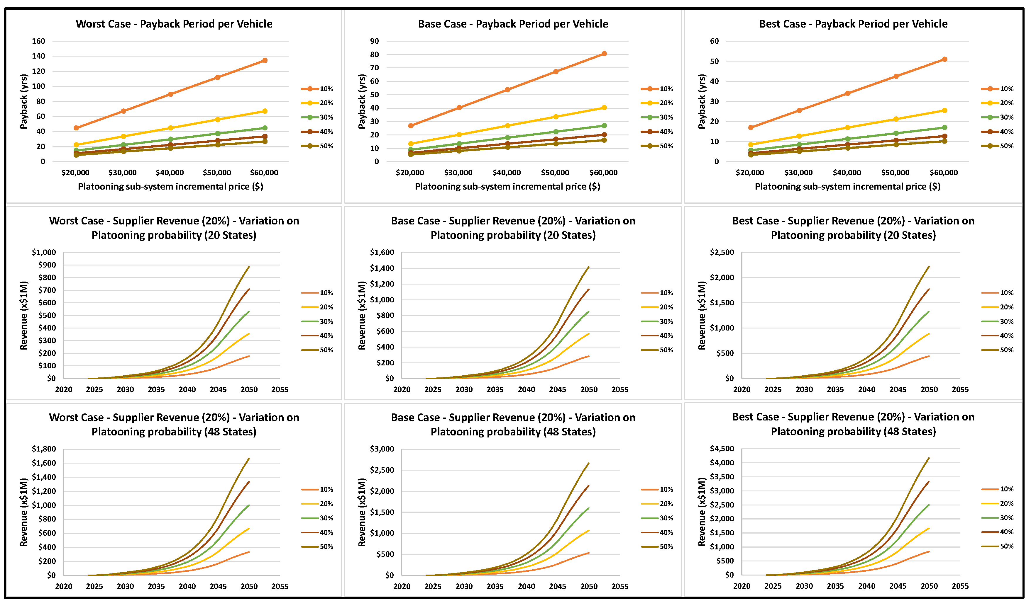
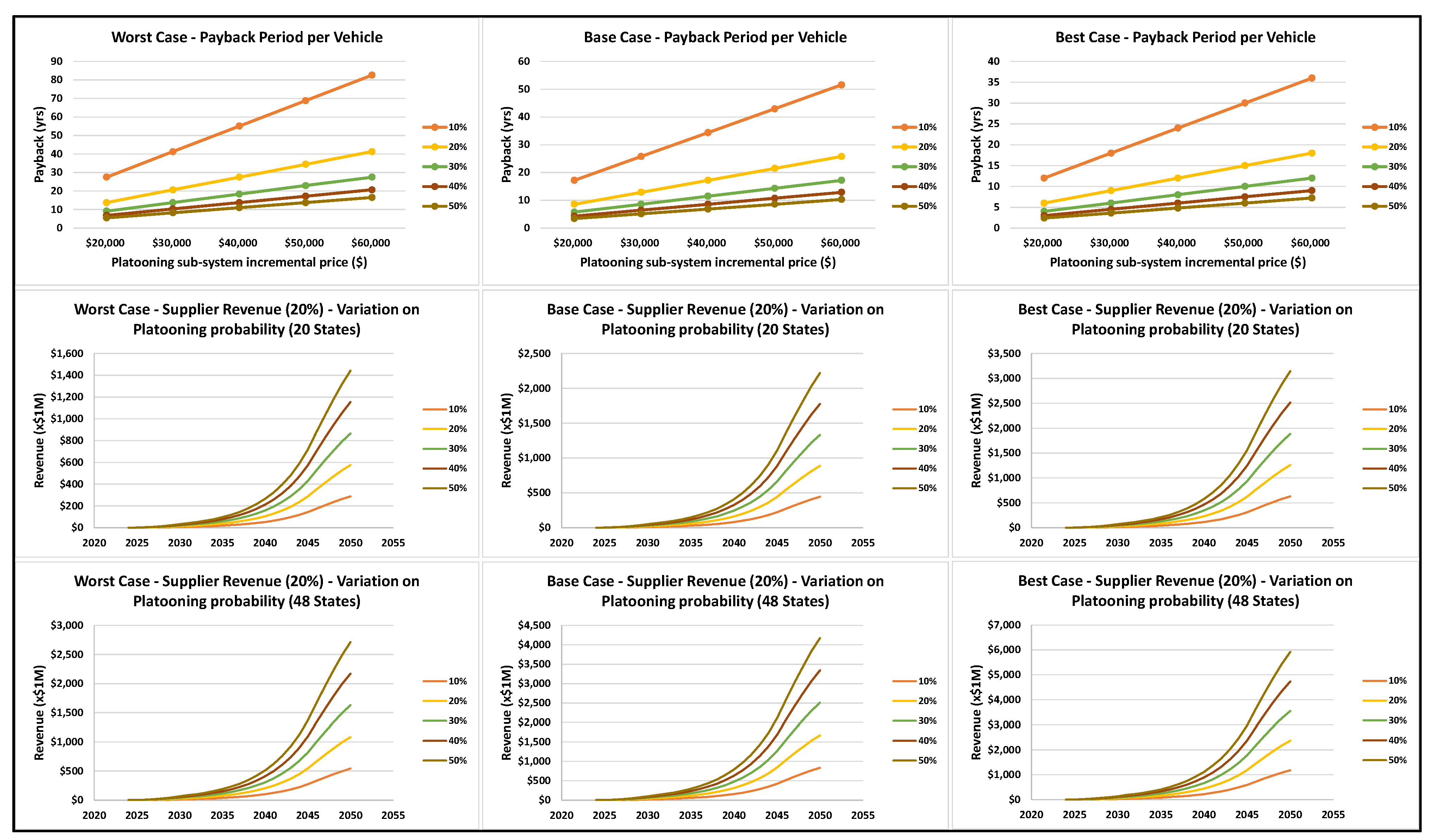
5.3. Scenario 3—Diesel v. BEV—Driver/Vehicle Hourly Value at Mean ($40.56/h)

In this scenario, the payback and revenue potential of an active platoon of 2 Class 8 tractor-trailers with diesel and electric powertrains (using the F&S adoption model) is assessed. Figure 34 and Figure 35 show the results for this. Here, the implications of the potential price of the added technology ($20,000 to $60,000), the probability of finding an active platooning partner (5% to 50%), the state regulation limits, the value of each additional hour of service is $40.56/h, the L4 operator resting equivalency factor is 0.25 (for each of hour of L4 rest, the operator gains 15 min of additional drive time) and the worst-case to best-case are shown. The main takeaways from this are the following:
  • Diesel payback: In the worst-case scenario, payback of ≤ 1.5 years occurs if either
    Technology price is $20,000 and probability of finding a platooning partner > 82.6%
    Technology price is $60,000 and probability of finding a platooning partner > 90.9%;
  • Diesel payback: In the best-case scenario, payback of ≤ 1.5 years occurs if either
    Technology price is $20,000 and probability of finding a platooning partner > 66.3%
    Technology price is $60,000 and probability of finding a platooning partner > 85.4%;
  • Diesel revenue: In the worst-case scenario, limited by current regulations (20 states) the revenue potential at:
    10 years of adoption will range from $8.0 M to $79.7 M
    20 years of adoption will range from $59.7 M to $597.3 M;
  • Diesel revenue: In the best-case scenario, unlimited by current regulations (48 states) the revenue potential at:
    10 years of adoption will range from $34.5 M to $344.8 M
    20 years of adoption will range from $249.5 M to $2495.4 M;
  • Electric payback: In the worst-case scenario, payback of ≤ 1.5 years occurs if either
    Technology price is $20,000 and probability of finding a platooning partner > 82.7%
    Technology price is $60,000 and probability of finding a platooning partner > 90.9%;
  • Electric payback: In the best-case scenario, payback of ≤ 1.5 years occurs if either
    Technology price is $20,000 and probability of finding a platooning partner >66.9 %
    Technology price is $60,000 and probability of finding a platooning partner > 85.6%;
  • Electric revenue: In the worst-case scenario, limited by current regulations (20 states) the revenue potential at:
    10 years of adoption will range from $7.9 M to $78.5 M
    20 years of adoption will range from $58.9 M to $588.7 M;
  • Electric revenue: In the best-case scenario, unlimited by current regulations (48 states) the revenue potential at:
    10 years of adoption will range from $33.8 M to $338.3 M
    20 years of adoption will range from $244.9 M to $2448.5 M.

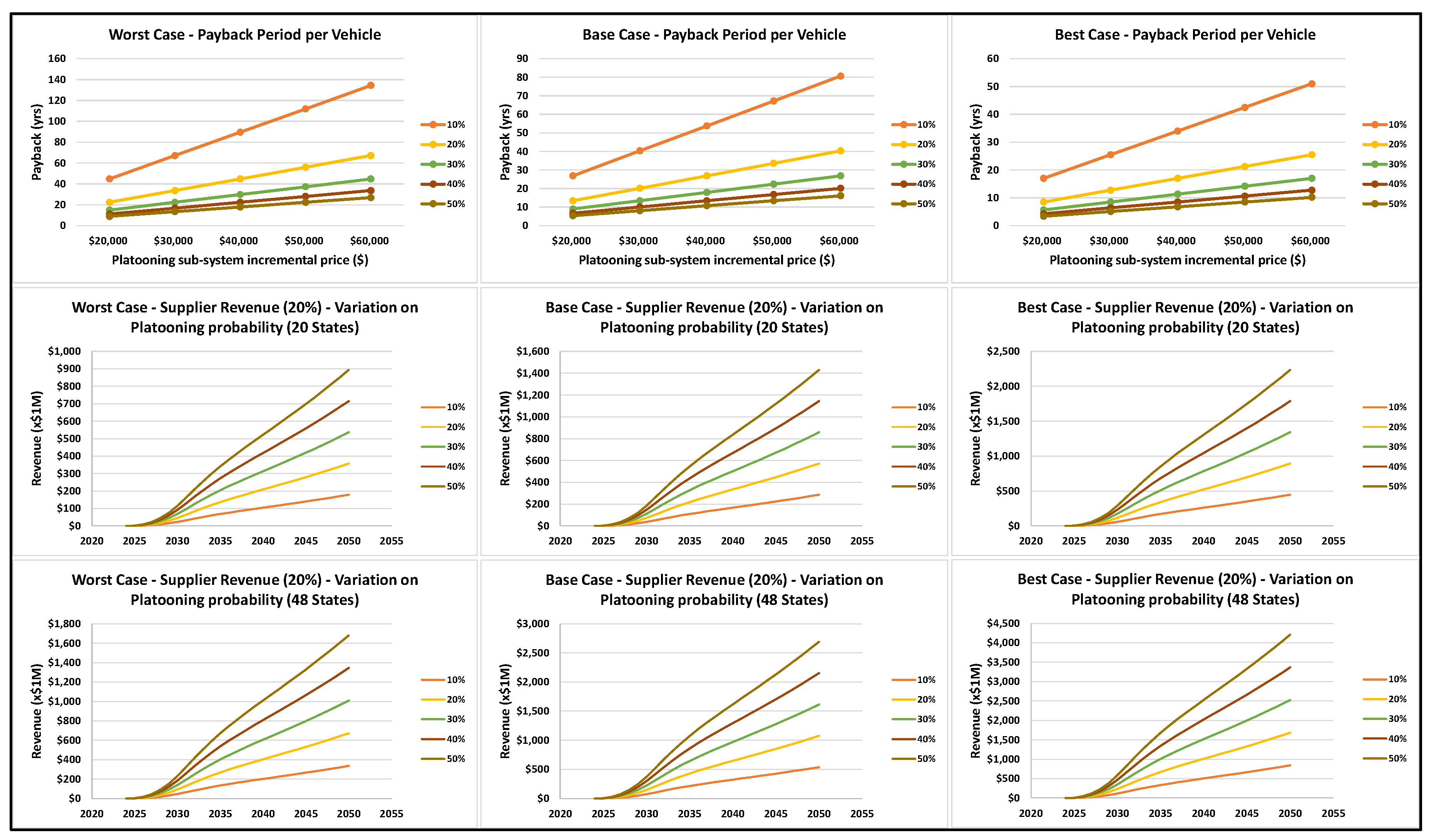
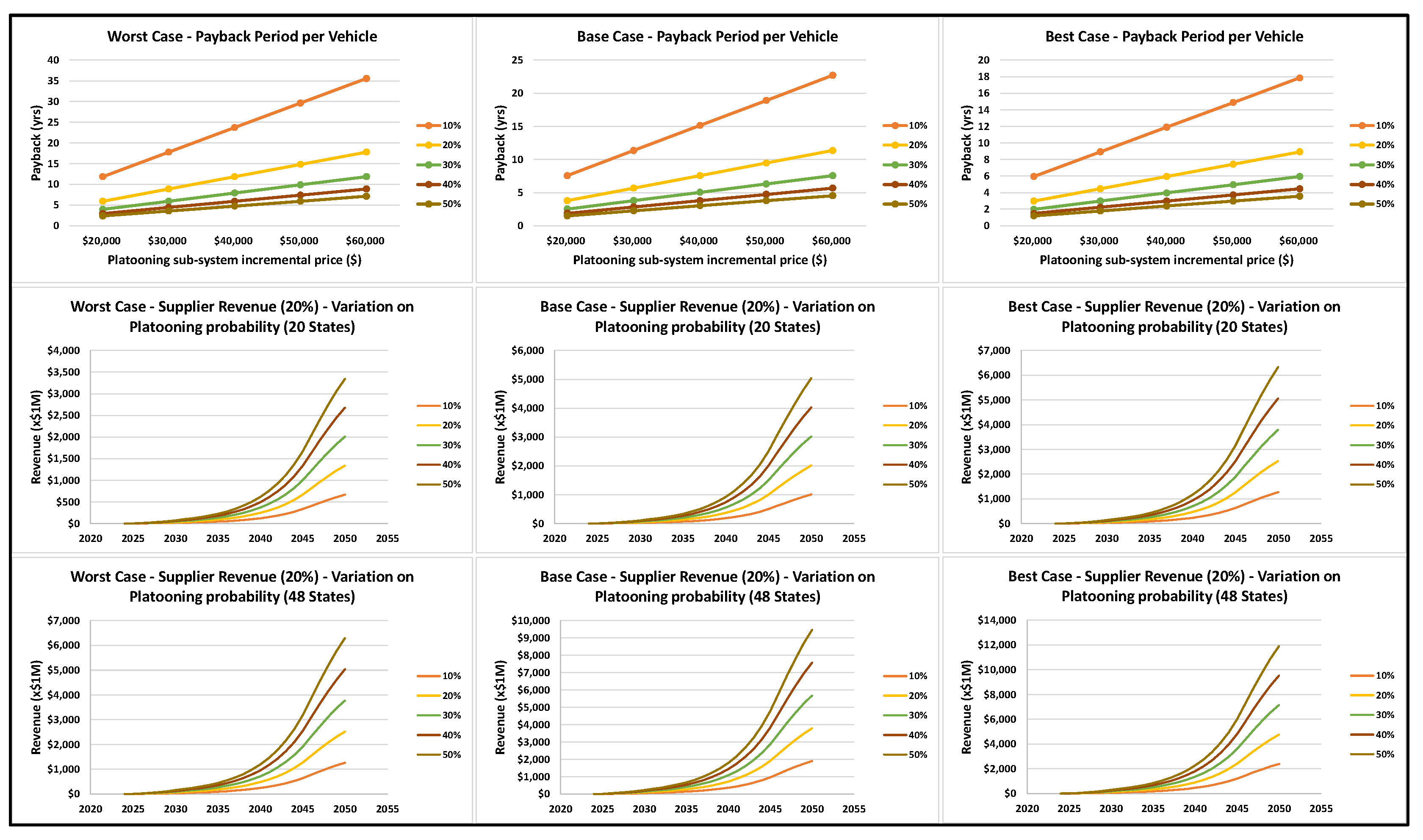
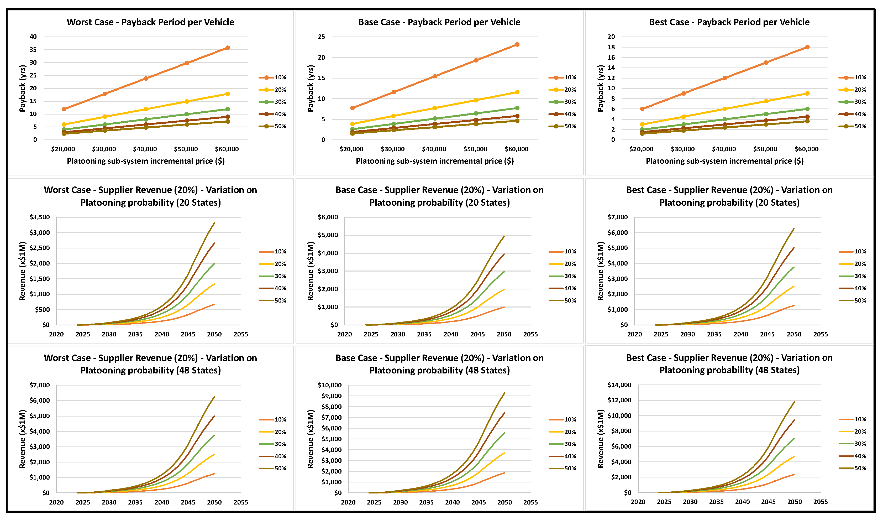
5.4. Scenario 4—Diesel v. BEV—High HoS Equivalency and Driver/Vehicle Hourly Value at Median ($24.09/h)

In this scenario, the payback and revenue potential of an active platoon of 2 Class 8 tractor-trailers with diesel and electric powertrains (using the F&S adoption model) is assessed. Figure 36 and Figure 37 show the results for this. Here, the implications of the potential price of the added technology ($20,000 to $60,000), the probability of finding an active platooning partner (5% to 50%), the state regulation limits, the value of each additional hour of service is $24.09/h, the L4 operator resting equivalency factor is 1 (for each of hour of L4 rest, the operator gains 60 min of additional drive time) and the worst-case to best-case are shown. The main takeaways from this are the following:
  • Diesel payback: In the worst-case scenario, payback of ≤ 1.5 years occurs if either
    Technology price is $20,000 and probability of finding a platooning partner > 66.5%
    Technology price is $60,000 and probability of finding a platooning partner > 85.5%;
  • Diesel payback: In the best-case scenario, payback of ≤ 1.5 years occurs if either
    Technology price is $20,000 and probability of finding a platooning partner > 39.7%
    Technology price is $60,000 and probability of finding a platooning partner > 76.1%;
  • Diesel revenue: In the worst-case scenario, limited by current regulations (20 states) the revenue potential at:
    10 years of adoption will range from $18.2 M to $182.3 M
    20 years of adoption will range from $136.6 M to $1366.5 M;
  • Diesel revenue: In the best-case scenario, unlimited by current regulations (48 states) the revenue potential at:
    10 years of adoption will range from $68.2 M to $681.9 M
    20 years of adoption will range from $493.6 M to $4935.7 M;
  • Electric payback: In the worst-case scenario, payback of ≤ 1.5 years occurs if either
    Technology price is $20,000 and probability of finding a platooning partner > 66.7%
    Technology price is $60,000 and probability of finding a platooning partner > 85.6%;
  • Electric payback: In the best-case scenario, payback of ≤ 1.5 years occurs if either
    Technology price is $20,000 and probability of finding a platooning partner > 40.1%
    Technology price is $60,000 and probability of finding a platooning partner > 76.3%;
  • Electric revenue: In the worst-case scenario, limited by current regulations (20 states) the revenue potential at:
    10 years of adoption will range from $18.1 M to $181.2 M
    20 years of adoption will range from $135.8 M to $1357.9 M;
  • Electric revenue: In the best-case scenario, unlimited by current regulations (48 states) the revenue potential at:
    10 years of adoption will range from $67.5 M to $675.4 M
    20 years of adoption will range from $488.9 M to $4888.8 M.

6. Summary Table of Key Results

The results presented in Section 5 are summarized here. The results above do not factor in traffic conditions and natural platooning that will occur. However, the expected payback (Table 3) and revenue potential (Table 4) shown here can be readily adjusted for the specific roads that the vehicle operated on (by reducing the platooning opportunities by the amount indicated in Figure 14). While several additional variants may be considered this study provides critical techno-economic guidance in the selection of active platooning for Class 8 tractor-trailer vehicles.
Table 3 shows the required probability of finding a platooning partner at different scenarios such that a payback of ≤ 1.5 years is achieved. Here, lighter-colored highlights are more appealing for near-term adoption—indicating payback of ≤ 1.5 years is possible with lower probability of finding a platooning partner. In other words, even with fewer platooning opportunities, it may be possible to achieve a viable payback. However, this is seen to occur at low-system technology price, best-case platooning assumptions, or high L4 operator resting equivalence factors. All of these present unique challenges on their own.
From Table 4, the more appealing regions of revenue potential are likewise highlighted with lighter colors. An interesting use-case where the operator is not present (either resting or otherwise) in the L4 vehicle is also shown. While the potential of these numbers is appealing, these also occur with base or best-case platooning assumptions, high L4 operator resting equivalence factors, more aggressive market adoption (Rogers model), higher platooning probabilities or greater state legislation supporting platooning. These present key challenges that will play into the realizability of the revenue potential.

7. Conclusions

Heavy duty vehicle platooning under highway operating conditions, has been projected to provide significant fuel economy gains based on aerodynamic drag improvements of the platooning vehicles. Realizing these benefits under real-world operating conditions presents several challenges. The objective of this paper (the third as part of a series) is to analytically quantify the payback and profitability of both conventional and electrified powertrains in heavy duty vehicles platooning across the US. Interstate highway system. In addition to the powertrain, key interactions that are explored include the market adoption rates, platooning velocities, platoon-able daily milage, platooning likelihood, variations in baseline powertrain fuel economy (diesel or electric), price of fuel (diesel or electricity), platooning fuel economy benefits, price of the added technology, and the impact of natural platooning due to traffic interactions. Further, the paper explores the economic impact of higher levels of vehicle automation for the trailing vehicles in the platoon, where extending the driver HoS may provide introduce additional financial benefits.
The assessment of the economic measures of active platooning explores several critical factors. These factors include: (i) powertrain type—diesel and electric, (ii) adoption model—Frost & Sullivan and Rogers, (iii) potential price of added technology—$500 to $2500, (iv) probability of finding an active platooning partner—5% to 50%, (v) state legislative constraints—20 states to all states, and (vi) scenarios for optimistic (best) case/base case/pessimistic (worst) case for platooning. The economic measures include end-user payback time (if technology is bought out complete) and a supplier revenue model (set at 20% of the savings potential based on a technology lease model of pay-per-use).
While the broad assessment of this space does reveal some promising pathways to achieve viable payback periods (≤1.5 years) and interesting revenue potential (>$500 M), realizing these present unique challenges that need to be considered carefully by both end-users and active platooning technology manufacturers/suppliers/producers. Due to the strong sensitivity of the economic model on driver HoS increases, research into the driver workload and rest effectiveness in a Level 4 platooning vehicle is recommended. Though many studies have extolled the possible impact of platooning, this paper series has addressed key challenges, requirements, and opportunities in realizing the benefits of platooning.

Author Contributions

Conceptualization, V.S. and P.T.J.; Data curation, V.S. and A.S.; Formal analysis, V.S.; Funding acquisition, V.S.; Investigation, V.S.; Methodology, V.S.; Project administration, V.S.; Resources, V.S.; Software, V.S.; Supervision, V.S.; Validation, V.S.; Visualization, V.S.; Writing—original draft, V.S.; Writing—review & editing, V.S., A.S. and P.T.J. All authors have read and agreed to the published version of the manuscript.

Funding

This research received no external funding.

Institutional Review Board Statement

Not applicable.

Informed Consent Statement

Not applicable.

Data Availability Statement

The data presented in this study are available on request from the corresponding author. All data generated and used in this study are summarized and referenced in the text of the document.

Conflicts of Interest

The authors declare no conflict of interest.

References

  1. Chadha, P.; Sujan, V. Quantification of Platooning Fuel Economy Benefits across United States Interstates Using Closed-Loop Vehicle Model Simulation. SAE Tech. Pap. 2021. [Google Scholar] [CrossRef]
  2. Sujan, V.; Vajapeyazula, P.; Kothandaraman, G.; Liu, J.; Follen, K. Platoon System for Vehicles. U.S. Patent 10,943,490, 9 March 2021. [Google Scholar]
  3. McAuliffe, B.; Lammert, M.; Lu, X.; Shladover, S. Influences on Energy Savings of Heavy Trucks Using Cooperative Adaptive Cruise Control. SAE Tech. Pap. 2018, 1, 1181. [Google Scholar] [CrossRef] [Green Version]
  4. Lammert, M.; Duran, A.; Diez, J.; Burton, K.; Nicholoson, A. Effect of Platooning on Fuel Consumption of Class 8 Vehicles Over a Range of Speeds, Following Distances, and Mass. SAE Int. J. Commer. Veh. 2014, 7, 626–639. [Google Scholar] [CrossRef] [Green Version]
  5. Eckerle, W.; Sujan, V.; Salemme, G. Future Challenges for Engine Manufacturers in View of Future Emissions Legislation. SAE Tech. Pap. 2017, 1, 1923. [Google Scholar] [CrossRef]
  6. Guerrero, A.; Davendralingam, N.; Raz, A.; DeLaurentis, D.; Shaver, G.; Sujan, V.; Jain, N. Projecting adoption of truck powertrain technologies and CO2 emissions in line-haul networks. Transp. Res. Part D Transp. Environ. 2020, 84, 102354. [Google Scholar] [CrossRef]
  7. Smith, J.; Mihelic, R.; Gifford, B.; Ellis, M. Aerodynamic Impact of Tractor-Trailer in Drafting Configuration. SAE Int. J. Commer. Veh. 2014, 7, 619–625. [Google Scholar] [CrossRef]
  8. USDOT, Federal Highway Administration. Exploratory Advanced Research (EAR) Program Fact Sheet: Expanding the Freight Capacity of America’s Highways; Report No. FHWA-HRT-17-045. USDOT; Federal Highway Administration: Washington, DC, USA, 2017. [Google Scholar]
  9. Sujan, V.; Jones, P.T.; Siekmann, A. Heavy Duty Commercial Vehicles Platooning Benefits for Conventional and Electrified Powertrains. In Proceedings of the IEEE International Conference on Connected Vehicles and Expo ICCVE, Lakeland, FL, USA, 7–9 March 2022. [Google Scholar]
  10. Sujan, V.; Jones, P.T.; Siekmann, A. Characterizing Minimum Admissible Separation Distances in Heavy Duty Vehicle Platoons. In Proceedings of the IEEE International Conference on Connected Vehicles and Expo ICCVE, Lakeland, FL, USA, 7–9 March 2022. [Google Scholar]
  11. Vahidi, A.; Sciarretta, A. Energy saving potentials of connected and automated vehicles. Transp. Res. C Emerg. Technol. 2018, 95, 822–843. [Google Scholar] [CrossRef]
  12. Mihelic, R. Fuel and Freight Efficiency–Past, Present and Future Perspectives. SAE Int. J. Commer. Veh. 2016, 9, 120–216. [Google Scholar] [CrossRef]
  13. Hussein, A.; Rakha, H. Vehicle Platooning Impact on Drag Coefficients and Energy/Fuel Saving Implications. Engineering, Computer Science, Environmental Science. arXiv 2020, arXiv:2001.00560. [Google Scholar]
  14. Salari, K.; Ortega, J. Experimental Investigation of the Aerodynamic Benefits of Truck Platooning. SAE Pap. 2018, 1, 0732. [Google Scholar] [CrossRef]
  15. McAuliffe, B.; Smith, P.; Raeesi, A.; Hoffman, M.; Bevly, D. Track-Based Aerodynamic Testing of a Two-Truck Platoon. SAE Int. J. Adv. Curr. Prac. Mobil. 2021, 3, 1450–1472. [Google Scholar]
  16. Ard, T.; Ashtiani, F.; Vahidi, A.; Borhan, H. Optimizing Gap Tracking Subject to Dynamic Losses via Connected and Anticipative MPC in Truck Platooning. In Proceedings of the 2020 American Control Conference (ACC), Denver, CO, USA, 1–3 July 2020; pp. 2300–2305. [Google Scholar]
  17. Shladover, S.E.; Nowakowski, C.; Lu, X.-Y. Using Cooperative Adaptive Cruise Control (CACC) to Form High-Performance Vehicle Streams. Definitions Literature Review and Operational Concept Alternatives; UC Berkeley: Berkeley, CA, USA, 2018. [Google Scholar]
  18. Devika, K.B.; Rohith, G.; Yellapantula, V.R.S.; Subramanian, S.C. A dynamics-based adaptive string stable controller for connected heavy road vehicle platoon safety. IEEE Access 2020, 8, 209. [Google Scholar] [CrossRef]
  19. Zhai, C.; Chen, X.; Yan, C.; Liu, Y.; Li, H. Ecological cooperative adaptive cruise control for a heterogeneous platoon of heavy-duty vehicles with time delays. IEEE Access 2020, 8, 146208–146219. [Google Scholar] [CrossRef]
  20. Guo, L.; Gao, B.; Gao, Y.; Chen, H. Optimal Energy Management for HEVs in Eco-Driving Applications Using Bi-Level MPC. IEEE Trans. Intell. Transp. Syst. 2017, 18, 2153–2162. [Google Scholar] [CrossRef]
  21. Yuniar, D.; Djakfar, L.; Wicaksono, A.; Efendi, A. Truck Driver Behavior and Travel Time Effectiveness Using Smart GPS. Civ. Eng. J. 2020, 6, 724–732. [Google Scholar] [CrossRef]
  22. Kapeller, H.; Dvorak, D.; Šimić, D. Improvement and Investigation of the Requirements for Electric Vehicles by the use of HVAC Modeling. HighTech Innov. J. 2021, 2, 67–76. [Google Scholar] [CrossRef]
  23. SAE International. J3016. Surface Vehicle Recommended Practice; SAE International: Warrendale, PA, USA, 1998. [Google Scholar]
  24. Marinik, A.; Bishop, R.; Fitchett, V.; Morgan, J.; Trimble, T.; Blanco, M. Human Factors Evaluation of Level 2 and Level 3 Automated Driving Concepts: Concepts of Operation; Report No. DOT HS 812 044; National Highway Traffic Safety Administration: Washington, DC, USA, 2015. [Google Scholar]
  25. U.S. Department of Transportation. Automated Vehicles: Truck Platooning ITS Benefits, Costs, and Lessons Learned: 2018 Update Report; Intelligent Transportation Systems Joint Program Office Report; U.S. Department of Transportation: Washington, DC, USA, 2018. [Google Scholar]
  26. Arkansas Trucking Association. ATRI Releases Results on Truck Platooning Study; Arkansas Trucking Association: Little Rock, AR, USA, 2015. [Google Scholar]
  27. U.S. Department of Transportation Federal Highway Administration. FHWA Research and Technology Evaluation: Truck Platooning, Final Report June 2021; Publication No. FHWA-HRT-20-071; U.S. Department of Transportation Federal Highway Administration: Washington, DC, USA, 2021. [Google Scholar]
  28. Vieth, K. Class 8 Review & Forecast. In Proceedings of the ACT Research Outlook Seminar 65, online, 24–26 August 2021. [Google Scholar]
  29. U.S. Department of Transportation Federal Highway Administration. FAF4 Network Database and Flow Assignment: 2012 and 2045. Available online: https://ops.fhwa.dot.gov/freight/freight_analysis/faf/faf4/netwkdbflow/index.htm (accessed on 10 October 2021).
  30. U.S. Department of Transportation—Federal Highway Administration. Available online: https://hepgis.fhwa.dot.gov/fhwagis/ (accessed on 6 January 2022).
  31. Law, S. Is Autonomous Truck Platooning Legal in Your State? Available online: https://simonlawpc.com/trucking-accident/autonomous-truck-platooning-legal-in-your-state/ (accessed on 31 October 2021).
  32. U.S. Department of Transportation Federal Highway Administration. Major Freight Corridors Map. Available online: https://ops.fhwa.dot.gov/freight/freight_analysis/nat_freight_stats/tonhwyrrww2012.htm (accessed on 6 January 2022).
  33. Here. Available online: https://www.here.com/ (accessed on 12 September 2021).
  34. Car and Driver. Drag Queens: Aerodynamics Compared. Available online: https://www.caranddriver.com/features/a15108689/drag-queens-aerodynamics-compared-comparison-test/ (accessed on 15 September 2021).
  35. Section 2–Aerodynamics. Available online: http://www.partnumber.com/ev/handbook/aerodynamics.html (accessed on 15 September 2021).
  36. Bishop, J. Table 2. Available online: https://www.researchgate.net/figure/Coefficient-of-drag-frontal-area-and-effective-drag-for-both-best-selling-and_tbl2_260994029 (accessed on 15 September 2021).
  37. Rogers, E.M. Diffusion of Innovations, 5th ed.; Free Press: New York, NY, USA, 2003; ISBN 0743222091. OCLC 782119567. [Google Scholar]
  38. PRNewswire. Truck Platooning Market Growth Opportunities 2016 to 2030 Autonomous Trucking Technologies to Launch Massive Productivity, Safety, and Efficiency Gains in Freight Mobility; Frost & Sullivan: San Antonio, TX, USA, 2016. [Google Scholar]
  39. Jacobs, J. What Does Disruptive Growth Look Like? Available online: https://www.globalxetfs.com/what-does-disruptive-growth-look-like/ (accessed on 2 November 2021).
  40. McGrath, R.G. The Pace of Technology Adoption is Speeding Up. Available online: https://hbr.org/2013/11/the-pace-of-technology-adoption-is-speeding-up/ (accessed on 2 November 2021).
  41. Fleet DNA Project Data. National Renewable Energy Laboratory. Available online: https://www.nrel.gov/fleetdna (accessed on 10 September 2021).
  42. TIGER/Line® Shapefiles. Available online: https://www.census.gov/cgi-bin/geo/shapefiles (accessed on 30 June 2021).
  43. Williams, N.; Murray, D. An Analysis of the Operational Costs of Trucking: 2020 Update; American Transportation Research Institute: Arlington, VA, USA, 2020. [Google Scholar]
  44. U.S. Energy Information Administration (EIA). Available online: https://www.eia.gov/ (accessed on 1 October 2021).
  45. Mericli, C. Development and Approach in Highly Automated Vehicles: Challenges and Opportunities—Technology Developer Perspective. In Proceedings of the Total Vehicle and Integration Committee, SAE Commercial Vehicles Engineering Congress (COMVEC), Chicago, IL, USA, 14 September 2021. [Google Scholar]
  46. Bruzelius, N. The Value of Travel Time; Croom Helm: London, UK, 1979. [Google Scholar]
  47. Haning, C.R.; McFarland, W.F. Value of Time Saved to Commercial Motor Vehicles Through Use of Improved Highways. A Report to the Bureau of Public Roads; Texas Transportation Institute: College Station, TX, USA, 1963. [Google Scholar]
  48. Adkins, W.G.; Ward, A.; McFarland, W.F. Value of Time Savings of Commercial Vehicles; HRB: Washington, DC, USA, 1967. [Google Scholar]
  49. Waters, W.G.; Wong, C.; Megale, K. The Value of Commercial Vehicle Time Savings for the Evaluation of Highway Investments: A Resource Saving Approach. J. Transp. Res. Forum 1995, 35, 97–113. [Google Scholar]
  50. Kawamura, K. Perceived Value of Time for Truck Operators. Transp. Res. Rec. J. Transp. Res. Board 2000, 1725, 31–36. [Google Scholar] [CrossRef]
  51. Smalkoski, B.; Levinson, D. Value of Time for Commercial Vehicle Operators. J. Transp. Res. Forum 2005, 44, 89–102. [Google Scholar] [CrossRef]
  52. Inflation Calculator. Available online: https://www.in2013dollars.com/us/inflation/ (accessed on 21 October 2021).
  53. Litman, T. Autonomous Vehicle Implementation Predictions Implications for Transport Planning. 2021. Available online: https://www.vtpi.org/avip.pdf (accessed on 6 January 2022).
Figure 1. Assimilation of observations on platooning drag based on literature [9].
Sustainability 14 02333 g001
Figure 2. Active Class 8 tractor population [28].
Sustainability 14 02333 g002
Figure 3. Class 8 tractor annual sales [28].
Sustainability 14 02333 g003
Figure 4. Class 8 active straight truck and tractor average age [28].
Sustainability 14 02333 g004
Figure 5. US interstate roads considered [30].
Sustainability 14 02333 g005
Figure 6. Major truck freight corridors and volume (roads, rail, and inland waterways) [32].
Sustainability 14 02333 g006
Figure 7. Class 8 active tractor count by each state for 2012 and 2045 based on FAF4. States that currently allow platooning are marked with dots (•) [31].
Sustainability 14 02333 g007
Figure 8. Interstate tractor-trailer (combination) truck count and density using FAF data [29].
Sustainability 14 02333 g008
Figure 9. Correlation between tractor-trailer truck count and truck density using FAF data [29].
Sustainability 14 02333 g009
Figure 10. Interstate Road speed limits distribution on all interstate highways using FAF data [29].
Sustainability 14 02333 g010
Figure 11. Class 8 truck and passenger car speed deviation from road speed limits on interstate highways [9].
Sustainability 14 02333 g011
Figure 12. Monte-Carlo results of natural platooning study.
Sustainability 14 02333 g012
Figure 13. Applying the results of the Class 8 tractor-trailer natural platooning Monte-Carlo study to the interstate highway truck distribution data from FAF to assess amount of natural platooning based on road mileage.
Sustainability 14 02333 g013
Figure 14. Applying the results of the Class 8 tractor-trailer natural platooning Monte-Carlo study to the interstate highway truck distribution data from FAF to assess amount of natural platooning based on truck count.
Sustainability 14 02333 g014
Figure 15. Theoretical adoption S-Curve of disruptive technologies [39].
Sustainability 14 02333 g015
Figure 16. Real adoption S-Curves of historical disruptive technologies [40].
Sustainability 14 02333 g016
Figure 17. Class 8 active tractor population annual usage miles [28,41].
Sustainability 14 02333 g017
Figure 18. Characterization of the two adoption models (Rogers and F&S) for active platooning.
Sustainability 14 02333 g018
Figure 19. HD routes mapped in Kinetic Intensity and Characteristic Velocity domain [9].
Sustainability 14 02333 g019
Figure 20. Single vehicle diesel fuel economy of 65 klb tractor-trailer with conventional powertrain (in miles per gallon and miles per kilowatt-hour).
Sustainability 14 02333 g020
Figure 21. Single vehicle electric fuel economy of 65 klb tractor-trailer with electric powertrain (in miles per diesel gallon equivalent and miles per kilowatt-hour).
Sustainability 14 02333 g021
Figure 22. Conventional powertrain—Active Platooning benefits—65 klbs—platooning FE gains (20 ft—red, 40 ft—blue, 75 ft—black) [9].
Sustainability 14 02333 g022
Figure 23. Electrified powertrain—Active Platooning benefits—65 klbs—platooning FE gains (20 ft—red, 40 ft—blue, 75 ft—black) [9].
Sustainability 14 02333 g023
Figure 24. Conventional powertrain—Active Platooning benefits—65 klbs—platooning fuel economy gains with traffic [9].
Sustainability 14 02333 g024
Figure 25. Electrified powertrain—Active Platooning benefits—65 klbs—platooning fuel economy gains with traffic [9].
Sustainability 14 02333 g025
Figure 26. Worst-case, base-case, and best-case payback and revenue potential for active platooning (with diesel powertrain, F&S adoption).
Sustainability 14 02333 g026
Figure 27. Worst-case, base-case, and best-case payback and revenue potential for active platooning (with electric powertrain, F&S adoption).
Sustainability 14 02333 g027
Figure 28. Worst-case, base-case, and best-case payback and revenue potential for active platooning (with diesel powertrain, Rogers adoption).
Sustainability 14 02333 g028
Figure 29. Worst-case, base-case, and best-case payback and revenue potential for active platooning (with electric powertrain, Rogers adoption).
Sustainability 14 02333 g029
Figure 30. Worst-case, base-case, and best-case payback and revenue potential for active platooning (with diesel powertrain, F&S adoption, driver HoS equivalency 0.25, driver/vehicle hourly value of $24.09/h).
Sustainability 14 02333 g030
Figure 31. Worst-case, base-case, and best-case payback and revenue potential for active platooning (with electric powertrain, F&S adoption, driver HoS equivalency 0.25, driver/vehicle hourly value of $24.09/h).
Sustainability 14 02333 g031
Figure 32. Worst-case, base-case, and best-case payback and revenue potential for active platooning (with diesel powertrain, Rogers adoption, driver HoS equivalency 0.25, driver/vehicle hourly value of $24.09/h).
Sustainability 14 02333 g032
Figure 33. Worst-case, base-case, and best-case payback and revenue potential for active platooning (with electric powertrain, Rogers adoption, driver HoS equivalency 0.25, driver/vehicle hourly value of $24.09/h).
Sustainability 14 02333 g033
Figure 34. Worst-case, base-case, and best-case payback and revenue potential for active platooning (with diesel powertrain, F&S adoption, driver HoS equivalency 0.25, driver/vehicle hourly value of $40.56/h).
Sustainability 14 02333 g034
Figure 35. Worst-case, base-case, and best-case payback and revenue potential for active platooning (with electric powertrain, F&S adoption, driver HoS equivalency 0.25, driver/vehicle hourly value of $40.56/h).
Sustainability 14 02333 g035
Figure 36. Worst-case, base-case, and best-case payback and revenue potential for active platooning (with diesel powertrain, F&S adoption, driver HoS equivalency 1, driver/vehicle hourly value of $24.09/h).
Sustainability 14 02333 g036
Figure 37. Worst-case, base-case, and best-case payback and revenue potential for active platooning (with electric powertrain, F&S adoption, driver HoS equivalency 1, driver/vehicle hourly value of $24.09/h).
Sustainability 14 02333 g037
Table 1. Worst-case, base-case, and best-case scenarios for active platooning (diesel power).
Worst CaseBase CaseBest Case
Platooning days per year286286286
Minimum daily miles to platoon (mi/day)300300300
Full fleet replacement cycle (yrs)666
Avg baseline FE (mpg or mi/kWh)9.007.756.50
Fuel cost ($/gal or $/kWh)2.53.55
Leading truck FE incr (%)4.0%6.5%9.0%
Trailing truck FE incr (%)4.0%6.5%9.0%
Fraction of Platoon-able miles (%)Miles/day30030%50%60%
35035%55%65%
40040%60%70%
45045%65%75%
50050%70%80%
Table 2. Worst-case, base-case, and best-case scenarios for active platooning (electrified power).
Worst CaseBase CaseBest Case
Platooning days per year286286286
Minimum daily miles to platoon (mi/day)300300300
Full fleet replacement cycle (yrs)666
Avg baseline FE (mpg or mi/kWh)0.440.380.32
Fuel cost ($/gal or $/kWh)0.070.10.2
Leading truck FE incr (%)5.5%8.0%10.5%
Trailing truck FE incr (%)5.5%8.0%10.5%
Fraction of Platoon-able miles (%)Miles/day30030%50%60%
35035%55%65%
40040%60%70%
45045%65%75%
50050%70%80%
Table 3. Summary of worst-case, base-case, and best-case scenarios for achieving viable payback in active platooning.
Payback Target: 1.5 yrs
ScenarioRequired Probability of Finding a Platooning Partner
Lead VehicleFollowing VehicleHourly Value ($/hr)L4 Operator Resting Equivalency FactorAdoption ModelPowertrainTech Price (LOW)Worst CaseBase CaseBest CaseTech Price (HIGH)Worst CaseBase CaseBest Case
L1L1 Diesel$50063.1%18.5%7.6%$250088.6%70.3%34.0%
Electric$50070.2%25.9%8.1%$250090.0%77.5%36.4%
L1L4$24.090.25 Diesel$20,00087.3%81.5%74.6%$60,00092.4%90.5%88.2%
Electric$20,00087.5%90.8%75.1%$60,00092.5%90.8%88.4%
$40.56 Diesel$20,00082.6%74.5%66.3%$60,00090.9%88.2%85.4%
Electric$20,00082.7%88.5%66.9%$60,00090.9%88.5%85.6%
$24.091.00 Diesel$20,00066.5%50.4%39.7%$60,00085.5%80.1%76.1%
Electric$20,00066.7%80.4%40.1%$60,00085.6%80.4%76.3%
$40.56 Diesel$20,00047.6%31.0%25.1%$60,00079.2%70.7%65.1%
Electric$20,00047.8%71.0%25.3%$60,00079.3%71.0%65.3%
$96.02 Diesel$20,00020.3%13.8%11.6%$60,00058.0%40.1%33.7%
Electric$20,00020.4%40.3%11.6%$60,00058.0%40.3%33.8%
Note: Probable use case when driver is not present in L4 vehicle, when hourly value are $40.56 or $96.02.
Table 4. Summary of worst-case, base-case, and best-case scenarios for achieving viable payback in active platooning.
ScenarioState Legislations Permit: 20 StatesState Legislations Permit: 48 States
Lead VehicleFollowing VehicleHourly Value ($/hr)L4 Operator Resting Equivalency FactorAdoption ModelPowertrainPlatooning ProbabilityWorst CaseBase CaseBest CaseWorst CaseBase CaseBest CaseWorst CaseBase CaseBest CaseWorst CaseBase CaseBest Case
%Revenue Potential @ 10 yrs (x$1,000,000)Revenue Potential @ 20 yrs (x$1,000,000)Revenue Potential @ 10 yrs (x$1,000,000)Revenue Potential @ 20 yrs (x$1,000,000)
L1L1 F&SDiesel5%$0.51$1.90$5.05$3.83$14.23$37.82$1.01$3.75$9.98$7.31$27.18$72.21
50%$5.11$18.99$50.46$38.28$142.34$378.19$10.10$37.55$99.76$73.10$271.76$722.07
Electric5%$0.40$1.34$4.72$2.97$10.07$35.36$0.78$2.66$9.33$5.67$19.22$67.52
50%$3.97$13.43$47.18$29.72$100.66$353.63$7.84$26.55$93.28$56.74$192.19$675.17
RogersDiesel5%$3.17$11.78$31.31$7.02$26.08$69.30$6.27$23.30$61.90$13.39$49.80$132.31
50%$31.69$117.83$313.07$70.15$260.83$693.01$62.66$232.96$618.96$133.94$497.98$1323.13
Electric5%$2.46$8.33$29.27$5.45$18.45$64.80$4.86$16.48$57.88$10.40$35.22$123.72
50%$24.60$83.33$292.73$54.46$184.46$648.00$48.64$164.75$578.76$103.98$352.18$1237.19
L1L4$24.090.25F&SDiesel5%$4.94$8.28$12.41$37.03$62.08$92.99$9.77$16.38$24.53$70.70$118.53$177.55
50%$49.41$82.83$124.07$370.33$620.84$929.93$97.69$163.77$245.30$707.05$1185.35$1775.47
Electric5%$4.83$7.73$12.08$36.18$57.92$90.54$9.54$15.28$23.88$69.07$110.58$172.86
50%$48.27$77.27$120.79$361.76$579.17$905.37$95.43$152.77$238.82$690.70$1105.78$1728.57
RogersDiesel5%$30.66$51.39$76.98$67.86$113.76$170.40$60.61$101.61$152.19$129.56$217.21$325.34
50%$306.56$513.93$769.79$678.59$1137.65$1704.02$606.08$1016.09$1521.94$1295.61$2172.06$3253.41
Electric5%$29.95$47.94$74.95$66.29$106.13$165.90$59.21$94.79$148.17$126.56$202.63$316.75
50%$299.47$479.44$749.46$662.90$1061.28$1659.01$592.07$947.88$1481.74$1265.65$2026.26$3167.47
$40.56F&SDiesel5%$7.97$12.65$17.44$59.73$94.79$130.70$15.75$25.00$34.48$114.03$180.97$249.54
50%$79.69$126.47$174.38$597.26$947.88$1307.02$157.55$250.03$344.77$1140.33$1809.74$2495.42
Electric5%$7.85$12.09$17.11$58.87$90.62$128.25$15.53$23.90$33.83$112.40$173.02$244.85
50%$78.54$120.91$171.10$588.70$906.21$1282.45$155.29$239.04$338.29$1123.97$1730.18$2448.52
RogersDiesel5%$49.44$78.47$108.19$109.44$173.69$239.50$97.75$155.13$213.91$208.96$331.62$457.27
50%$494.41$784.65$1081.95$1094.44$1736.91$2395.00$977.49$1551.32$2139.09$2089.55$3316.21$4572.66
Electric5%$48.73$75.02$106.16$107.87$166.05$235.00$96.35$148.31$209.89$205.96$317.04$448.67
50%$487.32$750.16$1061.61$1078.74$1660.55$2349.99$963.47$1483.11$2098.88$2059.59$3170.41$4486.72
$24.091.00F&SDiesel5%$18.23$27.44$34.49$136.65$205.64$258.51$36.04$54.24$68.19$260.89$392.61$493.57
50%$182.31$274.36$344.91$1366.45$2056.36$2585.14$360.44$542.43$681.91$2608.91$3926.11$4935.68
Electric5%$18.12$26.88$34.16$135.79$201.47$256.06$35.82$53.14$67.54$259.26$384.65$488.88
50%$181.17$268.80$341.63$1357.89$2014.69$2560.58$358.18$531.43$675.43$2592.55$3846.54$4888.79
RogersDiesel5%$113.11$170.23$214.00$250.39$376.81$473.71$223.64$336.55$423.09$478.06$719.43$904.42
50%$1131.15$1702.25$2139.97$2503.92$3768.11$4737.06$2236.36$3365.48$4230.89$4780.61$7194.28$9044.24
Electric5%$112.41$166.78$211.96$248.82$369.17$469.20$222.23$329.73$419.07$475.06$704.85$895.83
50%$1124.06$1667.75$2119.64$2488.22$3691.75$4692.05$2222.35$3297.27$4190.68$4750.65$7048.48$8958.30
$40.56F&SDiesel5%$30.34$44.89$54.62$227.42$336.45$409.35$59.99$88.75$107.98$434.20$642.37$781.55
50%$303.42$448.89$546.15$2274.20$3364.50$4093.48$599.89$887.49$1079.78$4342.01$6423.69$7815.50
Electric5%$30.23$44.33$54.29$226.56$332.28$406.89$59.76$87.65$107.33$432.57$634.41$776.86
50%$302.28$443.33$542.87$2265.63$3322.83$4068.92$597.63$876.50$1073.30$4325.66$6344.12$7768.60
RogersDiesel5%$188.26$278.51$338.86$416.73$616.52$750.10$372.20$550.64$669.95$795.64$1177.09$1432.13
50%$1882.58$2785.13$3388.58$4167.28$6165.18$7500.98$3721.99$5506.41$6699.47$7956.39$11,770.89$14,321.26
Electric5%$187.55$275.06$336.82$415.16$608.88$745.60$370.80$543.82$665.93$792.64$1162.51$1423.53
50%$1875.49$2750.63$3368.25$4151.59$6088.82$7455.97$3707.97$5438.20$6659.27$7926.43$11,625.09$14,235.32
$96.02F&SDiesel5%$71.14$103.68$122.40$533.19$777.09$917.42$140.64$204.98$242.00$1017.99$1483.66$1751.59
50%$711.37$1036.79$1224.02$5331.85$7770.88$9174.23$1406.44$2049.81$2419.98$10,179.85$14,836.58$17,515.91
Electric5%$71.02$103.12$122.07$532.33$772.92$914.97$140.42$203.88$241.35$1016.35$1475.70$1746.90
50%$710.23$1031.23$1220.74$5323.29$7729.21$9149.66$1404.18$2038.81$2413.50$10,163.50$14,757.01$17,469.01
RogersDiesel5%$441.37$643.27$759.44$977.02$1423.95$1681.10$872.62$1271.80$1501.47$1865.38$2718.68$3209.65
50%$4413.70$6432.73$7594.41$9770.19$14,239.51$16,811.02$8726.21$12,717.97$15,014.70$18,653.75$27,186.83$32,096.49
Electric5%$440.66$639.82$757.41$975.45$1416.31$1676.60$871.22$1264.98$1497.45$1862.38$2704.10$3201.06
50%$4406.61$6398.23$7574.08$9754.49$14,163.15$16,766.01$8712.19$12,649.76$14,974.50$18,623.79$27,041.03$32,010.55
Note: Probable use case when driver is not present in L4 vehicle, when hourly value are $40.56 or $96.02.
Publisher’s Note: MDPI stays neutral with regard to jurisdictional claims in published maps and institutional affiliations.

