Immunology-Based Sustainable Portfolio Management

Abstract

Immunological principles can be used to build a sustainable investment portfolio. The theory of immunology states that information about recognized pathogens is stored in the memory of the immune system. Information about previous illnesses can be helpful when the pathogen re-enters the body. Real-time analysis of 11 automated financial trading datasets confirmed this phenomenon in financial time series. Therefore, in order to increase the sustainability of the portfolio, we propose to train the portfolio with the most similar segments of historical data. The segment size and offset may vary depending on the data set and time.

1. Introduction

Important features of the modern world are constant changes taking place in economy, climate, finance and the need to process a huge amount of chaotic information. Automated financial trading is an excellent example of this. Here, we confront large-scale problems where thousands of traders use a variety of trading strategies.

When dealing with sustainability in financial trading, the main aim is “how to provide the opportunity for complex systems to be almost always reliable and survivable during its overall life cycle” [1]. A large number of different “improvements” were proposed to fulfil the portfolio designers’ dreams. Authors in their literature review [2] on sustainability, indicated that a general portfolio setting followed selection criteria and the company ’s strategies, which are usually based on management elements, e.g., time, cost, risk, quality, etc., leaving the sustainability variables behind. The following are a couple of examples. Zinovev, P. A., and Ismagilov proposed to use the Fuzzy forecasting technique, and ref. [3] suggested a sustainable collaboration of alliance of diverse portfolios. Furthermore, ref. [4] concluded that two main criteria should be used as parameters for quantifying portfolio sustainability: portfolio return and portfolio risk, with preference towards risk [5] using long-term memory (LSTM) networks [6] that are ideal for learning classification, time series processing and prediction problems, where important events are separated by indefinite time and boundary time intervals.

Due to the increasing complexity and non-convexity of financial engineering problems, biologically inspired heuristic algorithms gained considerable importance, especially in the area of financial decision optimization [7]. The use of artificial immune systems (AIS) is one of the heuristic algorithms [8]. An important procedure of AIS, called “negative selection“, is widely used in modern intrusion detection algorithms. This algorithm started to be used to speed up the calculation components of financial portfolios [9].

The immune system (IS) of vertebrates has a memory that stores information about the structure of previous pathogens (viruses, bacteria, etc.). Information about this structure enables the body to produce antibodies (molecules that interact with pathogens and help destroy them). As soon as antigens (invaders) appear, they are quickly destroyed (secondary immune response). Thus, the information stored in the immune memory about previously encountered antigens can be very useful [1]. 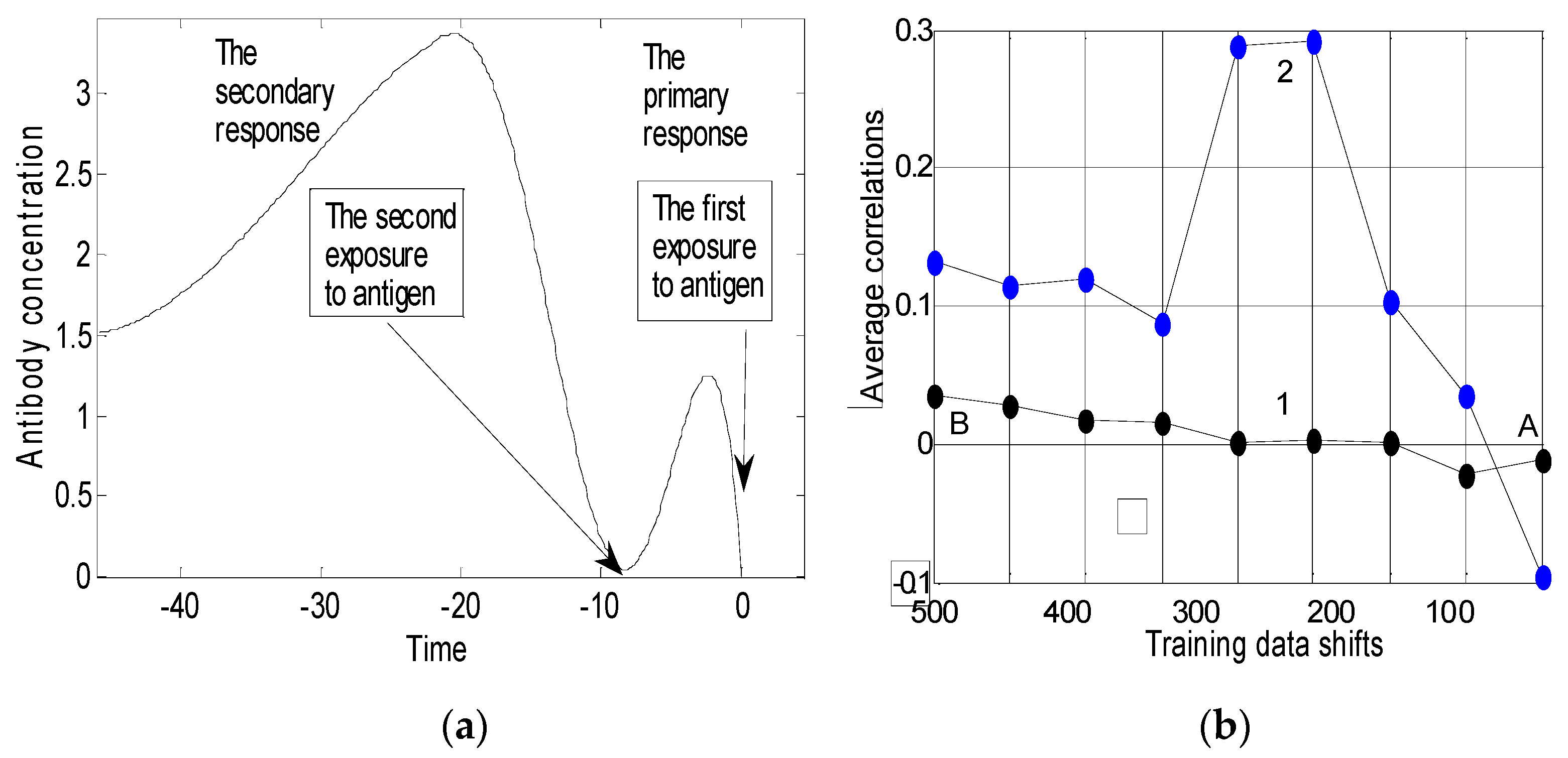Figure 1a, frequently used in immunology literature, shows that the secondary immune response is much stronger than the primary one. We see a small reaction of the immune system if the antigen appears for the first time. If the antigen appears a second time, the reaction is much stronger. This increases survivability and makes the population more sustainable.

Long-term sustainability is related to the concept of durability. Therefore, when we investigate sustainability issues, we must examine long time series of multivariate financial data. We speculate that there may be short sections of data in the long financial history, which, like a secondary immune target, can be used to calculate the portfolio weights and improve financial sustainability.

The goal of our article is not to create the best financial portfolio but to explore how to make better use of available historical data and select the segment of historical data to build the current portfolio. Hence, the two tasks of the article are as follows:

• To find a recurrence of similar segments in seemingly chaotic historical data;
• If we find this similarity, we can use this knowledge to improve the sustainability of the portfolio.

To the best of our knowledge, this kind of research has not been conducted before, and this is the scientific novelty of the present article.

Frequent changes in political, economic and financial factors make training sets too short for portfolio design with high-dimensional data [9,10]. Only a fraction of the most recent historical financial data can be used to find association rules in portfolio design in the belief that the most recent trends will persist over the next period of time.

In our previous article [11], we examined long time series of multivariate financial data and searched for the ‘optimal’ length of training data history. We found that the optimal length of history training in everyday trading depends on the specifics of the data and varies over time. An algorithm for the calculation of the length of learning history was proposed in [11]. We will also look into day-to-day trading where one or more significant changes in the environment may occur several times a year. Smaller changes take place every day. In our analysis, we consider extremely high-dimensional financial data (hundreds of thousands) aimed at creating a 1/N (equally weighted) portfolio. To have a profitable trade, the history of the j-th investment, r_ji, profit or loss (usually called returns) at the i-th point in time (month, day, etc.) is used to determine the proportions (weights) of investments, w_j, j = 1, 2, …, N. In the 1/N portfolio, all components of the portfolio, w_j, are equal: w_j = 1/N_similarity.

A classical method to calculate the portfolio weights is the “mean/variance quality criterion” [12,13]. In this approach, the Sharpe ratio is maximized:

SharpeR = mean(P(r))/variance(P(r)).

(1)

To calculate the portfolio weights, the mean and covariance matrix from training data, L N-dimensional training vectors r_i (i = 1 2, …, L), are to be estimated. The mean-variance approach is fruitful if the distribution of portfolio returns is Gaussian and the sample size/dimensionality ratio is large. Very often this ratio is small.

In trading, one deals with assets, stocks, bonds, and commodities. In advanced automated trading considered in the present paper, the profit and losses (PNL) of automated trading strategies (TS) are employed [14,15]. In sustainable portfolio management systems [16,17], one considers a vast variety of heuristically designed trading strategies and selects a single one or a small number of them capable of obtaining profit during the forthcoming period. Trading strategies (trading robots) mimic human psychology, knowledge and expertise. Histories of their outputs can contain useful additional information [16,17,18].

The number of trading strategies is constantly increasing. Presently, we are faced with tasks where the number of strategies reaches hundreds of thousands. The portfolio design schemas based on the mean-variance approach become worthless when the dimensionality of portfolio inputs exceeds the number of observations by hundreds of times. The selection accuracy of a small number of the best strategies becomes inexact when the training set size, L, is small. Hence, in the design, the proper portfolio rule problem, “selection of the appropriate subset of trading strategies”, becomes of great importance.

In an attempt to find novel solutions, we started examining nature’s information processing schemas aimed at maintaining sustainable human life. It was immunology that suggested a good idea. The vertebrate immune system has a memory that stores information about previous infections. Therefore, following a recurrent infection of the same type, healing is much faster. As the evolution of the immune system takes half a billion years, it might be considered to be a very important law of nature. The assessment of the old data also resembles the rules for making decisions on the nearest neighbor used in climatology, agriculture [19] and “structural dependence” in behavioral economics [17], where historians sometimes talk about repeating old historical events. The designers of an intrusion detection system noticed this innate property of vertebrates and started a new field of research called artificial immune systems [20,21]. The knowledge of artificial immune systems has already been applied to speed up the large-scale portfolio selection [9].

In the current article, we analyze the usefulness of historical information that can be helpful to portfolio design.

This paper is organized as follows. In Section 2, the main objective of the paper is presented: the necessity to use a lagged interval of historical data to select a profitable subset of trading systems for portfolio design. Section 3 and Section 4 describe the verification of the lagged training data principle by analyzing 11 financial data sets practically employed in automated trading. Section 5 concludes the paper.

2. Backward Shift of Training Data

Figure 1b (blue curve No. 2) shows that the secondary immune response [22] can be observed in real financial trading (details at the end of this Section).

To track the presence of the secondary reaction in financial trading, we analyzed one of the real multivariate time series of automatic day trading used in previous experiments [11]. The dimension of the data was N_data = 19,441 trading strategies, and the length of the data was L = 600 working days (approximately two years). We will name these data “selection history”. The aim was to assess which section of the selection history could be most informative to developing an N-dimensional portfolio that should be used for trading over the last 100 days (501:600). In this experiment, we chose the following dimension of the portfolio: N_similarity = 600 << N_data. Thus, in this experiment, the selection of the best 600 trading strategies out of 19,441 becomes an integral part of the portfolio management process.

To find the most informative segment of the training data, we divided the first 500-day data into 9 overlapping sections: (1:100), (51:150), …, (351:450), (401:500). The (501:600) working days served as a test set. The length of each section was l_sect = 100. The N_similarity/l_sect ratio is seen be seen to be very high. Therefore, we followed the recommendations of DeMiguel et al. [23,24]. We built 10 1/N portfolios for all 10 sections. In this way, we obtained 10 financial portfolios and used them to trade during the 100 test days. As a result, we obtained 10 N_similarity-dimensional return vectors, R₁, R₂, …, R₁₀, later to be used for finding the most informative segment of the training data.

To see the secondary effect in the resulting return vectors, we looked for similarities between vector R₁₀ and vectors: R₁, R₂, …, R₉. We plotted the distribution of R_j values relative to R₁₀ values on two-dimensional plots on the screen and also calculated the correlation coefficients between vectors R₁₀ and R_j (j = 1:9). Figure 1b contains graph 1 showing the dependence of the correlation coefficient on the lag value (in days). The effect is very small.

Increasing the Specificity of Trading Strategies

A possible reason for the lack of a clear secondary reaction is the low specificity of trading strategies. To increase specificity, we changed the display of data for available trading strategies:

• To reduce the impact of large fluctuations of returns, we used a square root transformation from the original data.
• Then, we used a 512-day history to compute the Fast Fourier Transform (FFT) weights.
• We used principal component analysis to reduce the size of the 512-day history of each trading strategy to 64.
• In this 64-dimensional space, we grouped 19, 411 64-dimensional vectors into 100 groups (clusters). Clustering is of help in accounting for many nonlinearities of multivariate distributions.
• To increase the specificity of the new sellers, we generated all possible, N_specifity = 100 × 99/2 = 4950 pairs from 100 average vectors (sellers1). The mean/variance method was used to obtain N_specifity of second-tier sales (sellers2), (see [25] for details).

Blue curve No. 2 in Figure 1b shows the dependence of the correlation, cor, on the lag for the new 4950-dimensional data. Here we see an obvious link between lagging and correlations. When a segment of validation data of 100 days follows a segment of the training data without any breaks, the lag = 100 days. The correlation is even negative (cor = −0.1). With a lag of 200–350 days, the correlation noticeably increases and approaches 0.3. Here, we see a “secondary response” that states that correctly shifted training data segments can be more useful than the most recent ones.

It should be noted that this is just one of the possible procedures designed to reveal the specificity of the trading strategies discussed in the current article.

3. Analysis of Multitude of Financial Time Series

The presence of a secondary reaction in financial trading data was analyzed above. The simplest parameter—variation in correlations—confirmed the idea of the secondary immune response. The analysis of a larger number of real multivariate time series will be presented below. A more detailed description of the data is provided in Appendix A.

Similar experiments were performed with 13,000-dimensional data D3 and 22,672-dimensional data D4. In both cases, we observed the presence of the secondary response in the study of correlations, the Sharpe ratio and portfolio returns. We see, again, that different lag durations vary. This confirms the assumption that when designing an adaptive financial portfolio, the most useful lag value should be determined individually for each time interval.

Analysis of the Sharpe Ratios

When analyzing correlation, we observed the secondary response effect (Figure 1b). We are interested in discovering if the secondary response effect is present in the Sharpe ratios and the portfolio returns.

To this end, we began to analyze the relationship between the portfolio performance and the lag. To characterize performance, we considered the following: (1) the Sharpe ratio of the two months sections of the selection history and (2) the 1/N (equally weighted) portfolio returns.

When speaking about natural immune systems, we emphasized that a high specificity of antibodies for a particular antigen was a very important factor. Hence, trading systems should be specific as well, able to trade perfectly even during a very short time period. Having an extremely large number of trading strategies, we believed them to be quite specific. Preliminary experiments confirmed this guess. To further increase the specificity of trading systems, we proposed the following method. We reduced the number of potential TSs by selecting only those that were effective for at least one two-month period during the last few years. This method was used in preparing data for the experiment reported in Section 2. This technique was used in this Section, too. The experimentally evaluated dependence of the Sharpe ratio values and the sums of the portfolio returns (both measured during two-month periods) on the lag of the training data segment are presented below (Figure 2a,b). We used a 26-month length section of 50,356-dimensional data D8 in that experiment. To increase the specificity of the trading strategies after the pre-selection procedure, dimensionality was reduced up to N_data = 29,920. In the experiment, the first 24 months were used to generate 23 two-month length sections used to find the secondary answer. The last 25 and 26 months were devoted to validation.

Both graphs in Figure 2 confirm the presence of the secondary response. The same effect on data D8 was also observed in the analysis of the correlations. To further examine these data, we defined the following parameters for D1, D5–D11 pre-screening and selection procedures to be used to analyze the datasets. Parameters include the length and dimension of the data chunks that will be used to select and test the best training data—two months and N_similarity = 600; in order to bring the new algorithm closer to practice, the number of trading systems used to calculate portfolio performance was reduced to n_fin = 30.

We used these parameters in the study of the mentioned datasets. For each data set, we were able to observe the phenomenon of the secondary response. We noticed that in all datasets, the most favorable lag values depended on the dataset. In addition, the optimal values could change over time.

4. Dynamic Lag-Based Portfolio

The ultimate goal of looking for secondary reaction phenomena in financial datasets is the desire to develop new adaptive sustainable portfolio management techniques that are immune to sudden changes in economy and the financial environment. The above study showed that the main parameter here was, without doubt, the size of the lag in the training data segment.

We have two years of training history. This history is divided into 23 intervals of 2 months, overlapping by 1 month. We use all history to determine the optimal lag. This optimal lag is used for the next 24th two-month period.

When testing the portfolio design algorithm, we selected the best lag value obtained during last month’s data. This scheme is a double out-of-sample strategy. Step 1: Data from 25 and 26 months are used to select similar trading strategies. Step 2: The following two months, i.e., 27 and 28, serve as a test set for the evaluation of the cumulative sum of portfolio returns.

Figure 3a represents a variation in the “optimal” lag during a six-year period in the experiments with data D11.

The two-month period (approximately 42 working days) allowed us to estimate the Sharpe ratio only approximately. We could see that optimal lag fluctuated too frequently (see Figure 3a). To reduce the fluctuations, we used smoothing. As a result, we obtained a moderate gain while calculating cumulative portfolio returns (sums of portfolio returns obtained during every single one-month shift of the data). We named this method the adaptive lag smoothing approach.

To be sure about the profitability of the adaptive lag smoothing approach, we performed simulation experiments with 11 real-world data sets, D1, D2, … D10 and D11. We used the method’s parameters obtained while working with data D8. The adaptive lag approach outperformed the “no-lag” method in the experiments with all data sets, with the exception of data D6. Gain ratio, the maximum of the cumulative sum of the adaptive lag approach divided by the maximum of the cumulative sum of the no-lag approach, is presented in the right-hand column of

Table A1. Real-world data considered in the paper.

	Length Months	Last Month	Noriginal	NFor Selection	Gain Ratio
D1	162	August 2016	60,314	9479	6.25
D2	135	February 2014	10,411	4950	1.10
D3	139	May 2014	13,000	4950	1.68
D4	143	September 2014	22,672	4950	1.33
D5	129	October 2015	15,473	14,719	2.23
D6	169	February 2017	29,049	17,511	0.83
D7	151	January 2016	47,501	19,306	1.13
D8	159	May 2016	50,356	29,920	3.96
D9	162	August 2016	60,314	36,697	4.36
D10	169	February 2017	65,827	17,472	1.42
D11	171	March 2017	127,838	15,913	1.43

. Figure 3b and Figure 4a–c show the cumulative function of the novel “adaptive smoothed lag Portfolio design scheme” obtained in the double out-of-samples experiment with data sets D11, D8, D6 and D5.

Figure 3b shows that the cumulative returns curve of the adaptive lag method outperforms the portfolio design scheme, where the test set follows the training set without a gap (in such case lag = 2 months). Five years after employing the novel method, a total gain in portfolio returns is almost four times larger than that when the method with lag = 2 was employed. Despite the use of the double out-of-sample strategy, the above result is too optimistic. The reason is the over-adaptation to data D8: We considered several modifications (diverse sets of the parameters) of the novel method and selected the best modification.

The graphs in Figure 3b and Figure 4a,b and Column 6 in Table A1 demonstrate the success achieved in the experiments with seven data sets. Figure 4c for data D6 shows success with the no-lag rule. Requests for details of data D6 preparation showed that, this time, trading strategies were selected in March 2017. It means that the 2011–February 2015 data were used in the training process. This factor spoiled the correct employment of the out-of-sample method. Therefore, this example is highly instructive.

Following our requirements, the inclusion of trading systems in data sets D1, D5, D7–D10 was performed until 2011 or 2013. These are earlier dates as compared to those of the beginning of the out-of-sample experimental tests. Moreover, 127,838-dimensional data D11 were prepared on 1 April 2017, without a preliminary pre-selection of trading strategies. It is no wonder the adaptive lag approach outperformed the “no-lag” strategy (see Figure 3b). On the very right-hand side of Figure 3b, we see a sudden fall in the value of the “no-lag” strategy (graph “lag = 2”). The analysis of the “adaptive lag” fluctuations on the right-hand side of Figure 3a can explain the reason for the ineffectiveness of the “no-lag” strategy.

5. Concluding Remarks

The two objectives of the article were as follows: (1) to find the presence of recurrence of similar segments in seemingly chaotic historical data; (2) if this similarity is found, can this knowledge be used to improve the sustainability of the portfolio? To the best of our knowledge, this kind of research has not been carried out before, and this is the novelty of our article.

In examining 11 multidimensional financial data sets, we noticed a recurrence of a similar historical data segment. We showed that by discovering the similarity to the section of training data, old data could be successfully used to build a new portfolio. It is necessary to find that section of data. If a similar history of training data was not observed, the financial portfolio could hardly have improved. This is very similar to the activity of the human immune system: O = If a person does not have X disease or has not been vaccinated, his/her resistance to X disease is low.

The goal of our article was not to create the “best” way to build a portfolio. When experimentally comparing the usefulness of multidimensional financial timeframes for the future portfolio formation, we merely noted the recurrence of similar situations in a half-million-year-old vertebrate immune system.

Repetition is a key feature of dynamic systems that can be used to describe the behaviors of a system in phase space. Recurrence plots [26] with their variations could be used in future research to determine the most appropriate historical data segment used to build the portfolio. Our transformation of financial time series using the Fast Fourier transform and data clustering described in Section 2 of the present paper allowed us to observe the cluster data structure.

The problem becomes more complicated when we deal with extremely high-dimensional time series. We are facing this type of difficulty at present. In the future, with the development of new technologies, we are sure to often encounter similar difficulties. In this article, we solve the automatic financial trading problem, where we can find large arrays of empirical data.

When considering the evolution of nature, we discovered that at least one problem of this type had already been solved. It is the vertebrate immune system with almost half a billion years of evolution. The study of the secondary immune response suggests that some previous historical evidence may be more informative. It is a serious argument that cannot be ignored.

A well-designed analysis of 11 real multidimensional financial trade data showed that the secondary response could be found in the financial time series. To apply this knowledge, it is necessary to find the most useful segment of historical financial time series data assigned to portfolio training. The optimal lag value depends on the data; it varies with time. In some times series, we cannot spot the secondary response effect. In principle, it is possible to find datasets where secondary response is absent. One should not expect the analysis of the previous period to be successful. We showed that simple averaging of success of previous lags could often improve portfolio performance.

The purpose of this article was to draw attention of the scientific community to the usefulness of the previously carefully selected training data segment in creating the investment portfolio. A prerequisite is that at least one range of historical data used for training would be similar to the current one. The fact that the specificity of trading strategies is high enough is also of great importance. More detailed and comprehensive studies are necessary in this field. In conclusion, it should be noted that repetition of similar data segments complicates the task of designing the sustainable portfolio management system, and these effects should not be ignored in practice.