Article

Spatiotemporal Variation in Gross Primary Productivity and Their Responses to Climate in the Great Lakes Region of Sub-Saharan Africa during 2001–2020

1
State Key Laboratory of Resource and Environmental Information System, Institute of Geographic Sciences and Natural Resources Research, Chinese Academy of Sciences, Beijing 100101, China
2
University of Chinese Academy of Sciences, Beijing 100049, China
3
School of Remote Sensing and Geomatics Engineering, Nanjing University of Information Science and Technology, Nanjing 210044, China
4
Institute of Atmospheric Composition and Environmental Meteorology, Chinese Academy of Meteorological Sciences, Beijing 100081, China
5
Jiangsu Center for Collaborative Innovation of Geographical Information Resources Development and Application, Nanjing 210023, China
6
Faculty of Sustainable Urban Planning and Development, University of Johannesburg, P.O. Box 17011, Doornfontein, Johannesburg 2028, South Africa
7
Aerospace Information Research Institute, Chinese Academy of Sciences, Beijing 100101, China
8
Rwanda Space Agency, Telecom House Kacyiru, Kigali P.O. Box 6205, Rwanda
*
Author to whom correspondence should be addressed.
Sustainability 2022, 14(5), 2610; https://doi.org/10.3390/su14052610
Submission received: 22 December 2021 / Revised: 26 January 2022 / Accepted: 11 February 2022 / Published: 24 February 2022

Abstract

:
The impacts of climate on spatiotemporal variations of eco-physiological and bio-physical factors have been widely explored in previous research, especially in dry areas. However, the understanding of gross primary productivity (GPP) variations and its interactions with climate in humid and semi-humid areas remains unclear. Based on hyperspectral satellite remotely sensed vegetation phenology processes and related indices and the re-analysed climate datasets, we investigated the seasonal and inter-annual variability of GPP by using different light-use efficiency (LUE) models including the Carnegie-Ames-Stanford Approaches (CASA) model, vegetation photosynthesis models (VPMChl and VPMCanopy) and Moderate Resolution Imaging Spectroradiometer (MODIS) GPP products (MOD17A2H) during 2001–2020 over the Great Lakes region of Sub-Saharan Africa (GLR-SSA). The models’ validation against the in situ GPP-based upscaled observations (GPP-EC) indicated that these three models can explain 82%, 79% and 80% of GPP variations with root mean square error (RMSE) values of 5.7, 8.82 and 10.12 g C·m−2·yr−1, respectively. The spatiotemporal variations of GPP showed that the GLR-SSA experienced: (i) high GPP values during December-May; (ii) high annual GPP increase during 2002–2003, 2011–2013 and 2015–2016 and annual decreasing with a marked alternation in other years; (iii) evergreen broadleaf forests having the highest GPP values while grasslands and croplands showing lower GPP values. The spatial correlation between GPP and climate factors indicated 60% relative correlation between precipitation and GPP and 65% correction between surface air temperature and GPP. The results also showed high GPP values under wet conditions (in rainy seasons and humid areas) that significantly fell by the rise of dry conditions (in long dry season and arid areas). Therefore, these results showed that climate factors have potential impact on GPP variability in this region. However, these findings may provide a better understanding of climate implications on GPP variability in the GLR-SSA and other tropical climate zones.

1. Introduction

Carbon uptake through the photosynthesis process by a terrestrial ecosystem termed gross primary productivity (GPP) [1,2] is the way CO2 enters into the biosphere from the atmosphere [3,4]. GPP not only drives the ecosystem functioning but also takes part in terrestrial carbon sequestration through phenological and physiological processes [5].
During the few past decades, some research has indicated that the accumulation rate of atmospheric CO2 has significantly increased and land and ocean sinks have exhibited a higher inter-annual variability. These changes in CO2 and sinks were significantly associated with the continuous major global climate change [1,2]. However, different diagnostic and prognostic models were developed and operated to estimate the spatial and temporal patterns of GPP variability [1,5,6,7].
These models are grouped into four categories based on their fundamental theories: enzymes kinetic process-based model, the light-use efficiency (LUE) or production efficiency models, machine learning models based on eddy covariance (EC), and other measurements statistically based on sun-induced chlorophyll fluorescence (SIF) models, respectively [7,8,9,10]. Among these approaches (models), the LUE models are widely used because of their simplicity of using the satellite-based production efficiency models (PEMs) and the capability of offering a relative balance at different spatial–temporal scales (hourly, daily, 8 days, 16 days, monthly and yearly; 250, 500 and 1000 m) [11,12,13].
LUE models are well understood at the leaf level and defined as the slope of the photosynthesis curve in the light-limited section [10]; hence, their initialization depends on variations from fractional photosynthesis active radiation (FPAR) through canopy and chlorophyll processes [6]. However, an accurate GPP estimation itself cannot provide accurate information about the ecosystem services to extreme climatic events but can help to predict future carbon cycle dynamics and their relationship to climate change [2,14]. Although the LUE models proved to be indispensable in GPP estimation, the comparison of different GPP-based models is more important to indicate the more reliable and higher accurate models for GPP simulations [15,16].
The application of GPP-based LUE models, especially in well-watered areas, provides a good understanding of how photosynthetic processes are regulated by ecosystem factors (biotic and abiotic) and climate factors, i.e., water availability (rainfall), temperature and other climate factors [6,7,16,17].
Over the past decades, multiple observations on the enhancement of seasonal and annual exchanges of CO2 and GPP variations, especially in the ecosystems induced by CO2 fertilization and with a limited extent of the growing season, were carried out from global to local scales. These variations of GPP indicated distinctive spatial pattern changes with climate in the hotspot ecosystems such as arid and grassland ecosystems [5,18,19]. Several research studies associated these changes with gradual variations in water availability and precipitation patterns [20,21].
However, the interactions between climate characteristics and GPP variations, particularly in humid and semi-humid climates, remain unclear. This study aimed at: (i) examining the spatial and temporal variation of GPP based on different LUE models and evaluating their stability on GPP simulations; (ii) evaluating the seasonal and inter-annual variations of GPP in different vegetation function types; and (iii) investigating the impacts of climate characteristics on GPP dynamics over the Great Lakes region of Sub-Saharan Africa (GLR-SSA).

2. Materials and Methods
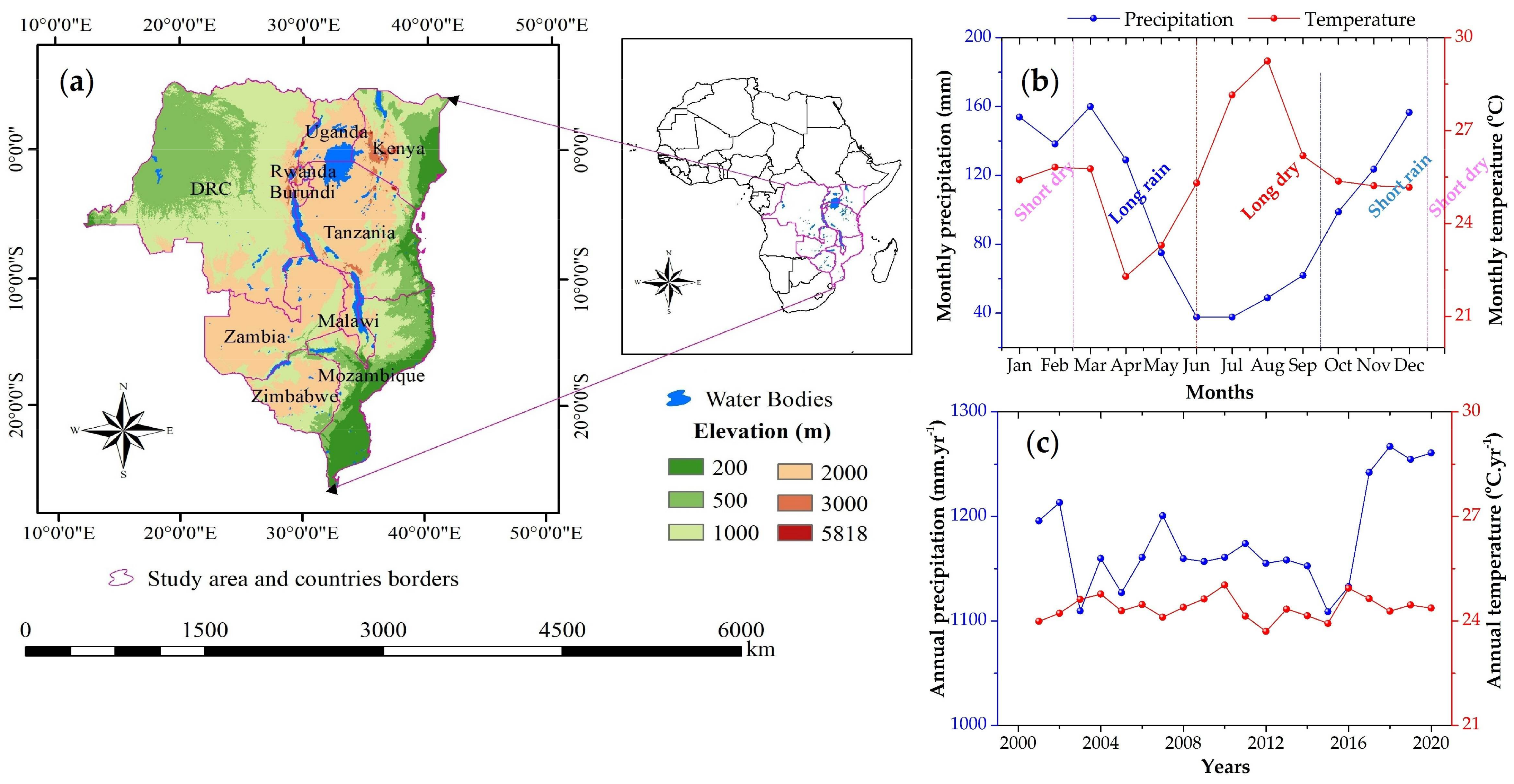
2.1. Study Area

This study was conducted in the Great Lakes region of Sub-Saharan Africa (GLR–SSA), occupying the surface area of approximately 6.3 million km2. This region extends over the African Great Lakes countries including the Democratic Republic of Congo (DRC), Burundi, Rwanda, Tanzania, Kenya and Uganda in east–central Africa and Zambia, Malawi, Mozambique and Zimbabwe in southern Africa. The European Space Agency Climate Change Initiative, Land Cover, ESA-CCI-LC [22], indicated that the major land cover types are: forest (~65.32%), cropland (~23.14%) and grassland (~7.42), while the other physical land cover (LC) types including built-up, wetlands, inland water and barren areas cover the remaining surface extent (~4.12%).
Köppen–Geiger climate types indicated that this region comprises ~70% of the African equatorial/tropical (T = 25 °C, P = 1170 mm yr−1), ~20% of sub-tropical (T = 24° C, P = 535 mm yr−1) and ~40% of temperate zones (T = 18 °C, P = 286 mm yr−1mm). The Climate Research Unit Time Series (CRU TS) land surface temperature datasets (2000–2020) indicate that this region consists of ~25 °C, ~1200 mm and ~650 mm of the overall annual average temperature, precipitation and evapotranspiration (ET), respectively [23,24]. This region also experiences four climatic seasons [25]: the two rainy seasons, namely, long rainy (late February to late May) and short rainy (end September to early December); and two dry seasons, namely, long dry (June–September) and short dry (mid-December to mid-February), respectively [26]. These two rainy seasons correspond to vegetation growing seasons due to the high precipitation occurrence [26,27]. The topographical elevation varies between 200 m in the lowest lands and plateau and 5818 m above sea level in the upper mountains (i.e., Mount Kilimanjaro) (Figure 1).
According to a soil atlas of Africa, the geospatial lithology and physical soil types of GLR–SSA are dominated by tropical and sub-tropical soil types features such as Acrisols (42%), Arenosols (19%), Chernozems (11%) and Greysol (4%); water bodies (8%); and other soil type features that make up the remaining 16% [28]. These diverse ecological patterns exert important influences on soil development and vegetation processes that may significantly contribute to carbon fluxes [26,29].

2.2. Datasets

GPP is a function of vegetation processes and climate variability. Hence, the performance of GPP variability considered the vegetation indices, vegetation status and climate factors at seasonal and inter-annual time series datasets, as illustrated in Table 1.

2.2.1. Vegetation Indices and Related Datasets

This study considered the MOD13A1, a 16-day composite normalized difference vegetation index (NDVI) derived from Moderate Resolution Imaging Spectroradiometer (MODIS); the MOD15A2H, an 8-day temporal resolution; a combined MODIS product which combines EVI (enhanced vegetation index), FPAR (faction of photosynthetically active radiation) and LAI (leaf area index) that represents the vegetation canopy; PAR data from Multi-angle Imaging SpectroRadiometer (MISR level 3), a Japanese global observation satellite product version 4 at daily composite; MCD12C1 version 6, yearly MODIS land cover (LC) data used to discriminate different dominated vegetation types (biomes) and other land cover classes and provide some model’s inputs constants and coefficients; and MOD09A1, an 8-day temporal resolution MODIS-Terra-based surface reflectance of soil water content or land surface water index (LWSI) data that were selected to represent the functional variations of shortwave infrared (SWIR) and near-infrared (NIR) electromagnetic spectrums [30]. This study also considered the MOD17A2H, a MODIS-based global GPP product version 6, at the cumulative of 8-days timescale and 500 m temporal and spatial resolutions. All of these data were acquired and freely downloaded from NASA Land Processes Distribution Active Archive Center (LP PAAC) distribution server as combined MODIS data pool and Earth-data for NASA’s Terra and Aqua satellite’s search engine websites as gridded products [31].

2.2.2. Climate Data

This study employed the filtered and spatially processed remotely sensed climate data such as the monthly precipitation and land surface air temperature (Tmean, Tmax and Tmin), which were freely downloaded from the Climate Engine data source powered by Google Earth Engine at 0.05° × 0.05° spatial resolution [32]. The other climate datasets used including soil moisture (SM), vapor pressure deficit (VPD), land surface temperature (LST), solar radiation (shortwave and longwave radiations), daily wind speed, potential evapotranspiration (PET) and evapotranspiration (ET) were acquired and freely downloaded from Terra Climate databases at 0.05° × 0.05° spatial resolutions [33]. These climate datasets were selected as GPP-LUE models’ climate inputs and used to estimate the aridity index and analyse the effects of climate characteristics on GPP variations.

2.2.3. Field-Based GPP Data for Models Performance Validation

Due to lack of and insufficient ground-based datasets in the GLR-SSA, this study considered GPP-based upscaled observations from the FLUXCOM ensemble of global land atmosphere energy and carbon fluxes as site-based data to validate the applied LUE models’ performances and simulated GPP results’ accuracy. These gridded carbon and energy fluxes data were merged from the global energy and carbon fluxes measurements simulated from the current global flux network (FLUXNET)-based eddy covariance (EC) towers, remote sensing and meteorological data by Martin Jung [34,35]. These well-processed GPP-EC data from 2001 to 2020 were freely obtained from the Max Planck Institute for Biogeochemistry’s website at 0.08° × 0.08° spatial resolution [36].

2.3. Methods

2.3.1. Data Processing

To analyse the seasonal and inter-annual spatiotemporal variations of GPP and climate variables, all the acquired gridded datasets were firstly re-projected to Africa Albers Equal Area Conic coordinate system to uniformly match geographical coordinates. Therefore, the obtained datasets for 8 and 16-day temporal resolutions were averaged to monthly and annually to match the objectives of this study. This study applied different light-use efficiency (LUE)-based models to estimate GPP. The LUE models proved to be realistic with hyperspectral satellite remotely sensed data and field spectrometer instruments from vegetation phenology processes [15]. All of the mean aggregated gridded datasets were re-sampled to 0.05° × 0.05° to match the spatial resolutions and smoothly harmonize the raster pixels by using the aggregated and focal statistics techniques in spatial analyst tools of ArcGis version 10.6 [16,37,38].
To consider the effects of different concepts of fraction photosynthetically active radiation absorbed by vegetation canopy (FPARCanopy) and fraction photosynthetically active radiation absorbed by vegetation chlorophyll (FPARChl), the vegetation photosynthesis model (VPM) was selected because of its excellency in estimating the relatively accurate GPP values [39]. Therefore, the VPM model was calibrated at vegetation canopy and chlorophyll levels as GPP-VPMCanopy and GPP-VPMChl respectively.
To ensure the significant comparison of GPP simulations at different LUE models, the Carnegie-Ames-Stanford Approach (CASA) model was also applied in this study to estimate GPP. The CASA model considers the individual biomes (plant function types or ecosystem types), maximum light-use efficiency (LUEmax or εmax) and NPP/GPP ratio of a variety of ecosystem types to simulate GPP [7]. To determine the CASA-based optimized ecosystem types (biomes) and related coefficients including σ ratio and maximum light-use efficiency (LUE, (ε)max), the MODIS land cover data (MCD12C1) provided in 16 land cover classes were reclassified into 8 classes according to the present dominated ecosystem types in the GLR-SSA (Figure 2).
Moreover, the modelled GPP results were validated against the FLUXCOM-based upscaled GPP values (GPP-EC) and compared with MODIS-GPP (MOD17A2H). In addition, climate characteristics including mean precipitation (Prec) and mean land surface air temperature (LST) were used to assess the impacts of seasonal and inter-annual climate variations on GPP dynamics. The entire data processing was performed in ENVI software version 5.6 (Exelis Visual Information Solutions, Inc., a subsidiary of Harris Corporation, Boulder, CO, USA) and ArcGIS software version 10.6 (Environment Systems Research Institute (Esri) Inc., Redlands, CA, USA); the two R packages, namely, package for autocorrelation robust testing-acrt version 1.0 suggested by Pötscher, B. M., and Preinerstorfer, D., 2018 [37] and Adaptive Smoothing of Digital Images-adimpro version 0.9.2 suggested by Polzehl, J., and Tabelow, K., 2006 [38]; and Origin-Pro version 9.0 software provided by OriginLab.

2.3.2. Descriptions of GPP Models

The CASA Model

The CASA model is a widely recognized LUE model for its capability to down-regulate photosynthetic efficiency in response to different vegetation, soil and climate conditions, and intercept solar radiation [7,40,41]. The CASA model was proposed by Monteith [41]. CASA model-based GPP was estimated monthly and annually under the following equation (Equation (1)):
G P P = N P P / σ
N P P x , t = A P A R x , t × ε x , t
where GPP is gross primary productivity (gC·m−2·timescale−1), t is timescale (monthly and yearly), and x is grid position [42]. NPP is net primary productivity (gC·m−2·timescale−1); σ is the ratio associated with different dominated biomes (Table 2).
A P A R x , t is absorbed photosynthetically active radiation measured in MJ·m−2 and ε x , t is light-use efficient (gC·MJ−1) [7]. A P A R x , t is determined in function with both solar radiation and the characteristics of the plant canopy and is calculated by this equation (Equation (3)).
  A P A R x , t = 0.5 × S o R x , t × f A P A R x , t  
S o R x , t stands for solar radiation (in MJ·m−2·timescale−1); f A P A R x , t is the fraction of APAR absorbed from plant canopy; and 0.5 indicates the proportion of radiation that can be absorbed by plants in range of 0.38–0.71 µm electromagnetic spectrum [7]. Therefore, f A P A R x , t was estimated based on the variations of NDVI [47] as the following equation (Equation (4)):
f A P A R x , t = N D V I x ,   t N D V I i ,   m i n × f A P A R m a x f A P A R m i n N D V I i , m a x N D V I i ,   m i n + f A P A R m i n
where N D V I i ,   m i n and N D V I i ,   m a x stand for minimum and maximum of vegetation type assigned 5% and 95% in the NDVI histogram; and f A P A R m a x f A P A R m i n are constant, with values 0.95 and 0.001, respectively [7]. ε is a function of climate factors such as temperature and vapor pressure deficit [48] and was calculated based on the following equation (Equation (5)).
ε x , t = T τ 1 x , t × T τ 2 x , t × w τ x , t × ε m a x
where T τ 1 , T τ 2 , w τ and ε m a x indicate the effects of low and high temperature, soil moisture and the maximum light-used applied on LUE. ε m a x   values in gC/mol·MJ−1 are provided in Table 2.

The VPM Model

The vegetation photosynthetic model (VPM) is one of the satellite-based production efficiency models (PEMs) that estimates GPP as the product of light absorbed by chlorophyll of the vegetation (APARChl) or vegetation canopy (APARCanopy) and efficiency εg to convert the absorbed energy to carbon fixed by plants through photosynthesis [17,37]. In this study, we have estimated GPP by considering these two above-stated vegetation phenological processes effects through the following equations (Equations (6) and (7)).
G P P V P M C h l = A P A R C h l × ε g
G P P V P M C a n o p y = A P A R C a n o p y × ε g
where A P A R C h l and A P A R C a n o p y were calculated from photosynthetically active radiation (PAR) and the fraction of PAR absorbed by chlorophyll and canopy, respectively [17], as shown in Equations (8) and (10).
A P A R C h l = P A R × f P A R C h l  
where f P A R C h l is calculated as a linear function of the enhance vegetation index (EVI), which was modified from a previous model framework [6,37].
f A P A R C h l = E V I 0.1 × 1.25
The coefficients 0.1 and 1.25 were used to adjust for sparse vegetation and nonvegetated area. The f P A R C a n o p y in this study was estimated to be equivalent to the leaf area index (LAI) or NDVI of the vegetation types in the GLR–SSA’s terrestrial ecosystem, as suggested by Pradeep Wagle [44].
A P A R C a n o p y = P A R × L A I c a n o p y  
The ε g   is a function of temperature limitation (Tscalar) and water stress (Wscalar) from its maximum value ε m a x , which was deriveds from different biomes (Table 2); the following equation (Equation (11)) is ε g estimation formula:
ε g = ε m a x × T s c a l a r × W s c a l a r
Both T s c a l a r   and W s c a l a r   range from 0 to 1, and they can be calculated as follows:
T s c a l a r = T T m a x × T T m i n T T m a x × T T m i n T T o p t 2
W s c a l a r = 1 + L S W I 1 + L S W I m a x
T is air temperature (°C); Tmin, Tmax and Topt are minimum, maximum and optimal temperature (°C) parameters for photosynthesis of each biome, respectively [16]. Their values are illustrated in the different biomes look-up table (Table 2). LSWImax is the maximum land surface water index at snow-free at each pixel and each timescale [37].

2.3.3. Estimation of Aridity Index

The aridity index (AI) was calculated as the ratio of potential evapotranspiration (PET) and precipitation (Prec) as defined by the Penman-Monteith [49] method (Equation (14)).
A I = P E T x , t P r e c x , t  
where P E T x , t stands for potential evapotranspiration (mm) and P r e c x , t for precipitation (mm) at timescale t and grid position x, respectively. The P E T x , t   was estimated by using the following equation (Equation (15)):
  P E T x , t = 0.408 Δ R n G + ρ 900 T a i r + 273 W s 2 e s e a Δ + ρ 1 + 0.34 W s 2
R n is the net radiation at the canopy (MJ·m−2·timescale−1), G is the soil heat flux density (MJ·m−2·timescale−1), which was calculated by the difference of mean daily air temperature between two continuous days as estimated by Penman-Monteith and by Thornthwaite [50,51] methods. T a i r stands for the mean daily air temperature at 2 m of height (°C), W s 2 is the wind speed at 2 m of height (m·s−1) and e s e a are the saturation and the actual vapor pressure (kPa), while Δ is the slope of saturated vapor pressure in relation to air temperature (kPa·°C−1) and ρ is the psychometric constant (kPa·°C−1), respectively. The R n was estimated from the difference between the net shortwave radiation (Rns) and the net longwave radiation (Rnl) (Equation (16)):
R n = R n s R n l
Generally, AI is expressed on the annual basis as the fact that the degree of dryness cannot be determined at daily or monthly time scales, which differentiates the aridity and drought concepts [21,51]. To optimize our AI estimation onto the GLR-SSA tropical climate [52], we have applied the mean annual values of PET and Prec to calculate the AI from 2001 to 2020. Moreover, the AI values were classified in accordance with UNEP and UNESCO aridity classification limits based on Thornthwaite (UNEP 1992) and Penman (UNESCO 1978) methods, respectively (Table 3 and Figure 3).
The GLR-SSA was dominated by humid climate (70%), while the other climate zones were extended over the remaining 30% of the GLR-SSA in which semi-humid, semi-arid and arid climate zones are extended over approximately 10%, 2.79% and 11.23%, respectively as the UNEP and UNESCO classifications (Figure 3).

2.3.4. Evaluation of Model Performance

The accuracy of modelled GPP results and the LUE models stability validation were assessed by comparing the resulted values with the upscaled GPP-EC [34] by using four coefficient measures including the R square (R2); root mean square error (RMSE); relative error (RE) and Bias. R2 was evaluated in range from −1 to 1, while RMSE, RE and Bias were calculated at the same unit with GPP (g C·m−2·yr−1) with the agreement that higher R2 and lower RMSE, RE and Bias implied higher accuracy and model stability [53].

2.3.5. The Analysis of Spatial Relationship between GPP with Climate Factors

To analyse the spatial relationship between GPP variability and local climate factors, the geographic weighted regression (GWR) model was employed. Modelling samples used to run the GWR model were developed based on pixels of the averaged mean annual GPP values from each GPP-LUE model results (CASA, GPP-VPM Canopy, GPP-VPM Chl) and the observed MODIS-GPP (MOD17A2H); and the averaged mean annual values of each climate factor (Prec and LST). GPP pixel values were selected as dependent variables, while climate factors were selected as independent variables. The GWR model was calibrated using the equation suggested by Xue Lin [54] (Equations (17) and (18)).
  y i = β 0 + k = 1 p β k x i k + ε i
  y i = β i 0 u j , v j + k = 1 p β i k u j , v j x i k + ε i
where y i is the dependent variable of ith sample, which represents GPP value at pixel i; x i k is the kth explanatory variable of the ith sample that denotes the climate factor (Prec or LST) value at pixel i; p is the total number of explanatory variables; β k is the coefficient of the kth explanatory variable; β 0 donates the intercept; ε i is the error term; u j   , v j represents the geographic coordinate of the ith sample. The estimated coefficients β i k for each sample vary depending on the associated location [54]. Finally, the GWR model results were selected in varieties of five GWR stepwise regressions based on the Pearson product moments correlation to verify the effects of climate factors to GPP variability at pixel level [55].

3. Results

3.1. The Spatial Patterns of GPP

The spatial pattern analysis indicated that during 2001–2020, the annual GPP in the GLR–SSA varied between 0 and 3000 g C·m−2·yr−1. High values of GPP were found in the lower plateau of the Democratic Republic of Congo (DRC) and the areas closer to Indian Ocean coastlines, while lower GPP values were obtained in the high mountain regions.
Both the modelled and observed GPP results indicated a concentration of higher GPP values ranging from 1500 to 3000 g C·m−2·yr−1 in the western parts of the study area, such as the DRC’s rainforests and surrounding ecosystems including the Congo Basin. Lower to optimal GPP concentration was obtained in higher mountains’ chain, forming the rift valley and the Nile ridge ecosystems and in the extended regions of the Kalahari Desert. These regions were characterized by GPP values ranging between 0 and 1200 g C·m−2·yr−1 during 2001–2020 (Figure 4).

3.2. Model Validation and GPP Simulation Stability

The model performance validation against GPP-EC indicated that the estimated GPP outputs were significantly correlated with GPP-EC (the verifier) with higher R2 values (p < 0.05), lesser RMSE and RE values and tolerable BIAS values according to O’Hara [56]. This assessment indicated a strong correlation (R2 = 0.88) between GPP–EC and GPP-CASA, followed by VPM Canopy model with the correction of R2 = 0.85 between GPP-EC and GPP–VPM Canopy. GPP-VPMChl and MOD17A2H values exhibited optimal and fair correlations with GPP-EC at R2 = 0.72 and R2 = 0.59, respectively. The CASA model indicated the lowest simulation error values among all the other employed LUE models, which indicates the indispensability of the CASA model to simulate GPP in the GLR-SSA and other tropical-related ecosystems. The model validation results and LUE models’ stability assessment results are illustrated in Figure 5.

3.3. Seasonal and Inter-Annual Variations in GPP during 2001–2016

An analysis of the seasonal and inter-annual GPP variations revealed that the mean monthly GPP varied between 15 and 180 g C·m−2·month−1. The seasons between December and May (Dec-Jan-Feb and Mar-Apr-May) were characterized by higher GPP values (≥80 g C·m−2·month−1). This analysis also indicted that seasonal–monthly GPP variation reached the peak values in February-March (≥160 g C·m−2·month−1). The mean annual GPP varied between 1000 and 1600 g C·m−2·yr−1. The optimal increases were observed during 2002–2003, 2011–2013 and 2015–2016: while decreasing trends were detected during 2006–2007, 2010–2011 and 2013–2014, the other periods were characterized by interchanges of decreases and increases over both the modelled and observed GPP estimates (Figure 6).

3.4. Analysis of GPP Variations among Individual Ecosystem Function Types (Biomes)

The analysis of GPP variations over the individual ecosystem function types (biomes) indicated an indispensable influence of each individual biome to GPP dynamics, confirming the effect of FPAR on GPP variability. The evergreen broadleaf (EVGB) represented the highest contribution to the GPP production through photosynthesis with significant peaks in all modelled approaches (CASA, VPMCanopy, VPMChl and MOD17A2H). The annual grass and crops exhibited the lowest photosynthetic activity ranging from 1.27 ± 0.36 g C·m−2·yr−1 to 45.41 ± 1.27 g C·m−2·yr−1, respectively, compared to all other dominating biomes in the GLR-SSA terrestrial ecosystem (Figure 7).
However, among the simulations results, the GPP-CASA results showed the highest mean GPP values for EVGB varied in the range from 246 to 375 g C·m−2·yr−1 with a standard deviation ranging from ± 1.54 to ± 6.14 g C·m−2·yr−1, and the annual GPP change rate ranged between −3.31 and 6.67g C·m−2·yr−1 compared to the other LUE models and the observed MODIS-GPP.

3.5. Spatial Variations of GPP in Response to Climate Factors

The spatial correlation GPP and precipitation indicated great influences of precipitation on the variability of GPP in GLR-SSA with 74.16%, 73.71%, 61.14% and 64.51% for GPP-VPMCanopy, GPP-VPMChl, GPP-MOD17 and GPP-CASA, respectively. The overall analysis indicated that spatially precipitation significantly induced the GPP variability for at least 60% of the GLR-SSA extent (Figure 8).
The overall analysis of spatial correlation between LST and GPP also indicated that LST and GPP were significantly correlated at 65% (Figure 7). The LST and GPP-MOD17 were correlated at 65.14%; LST and GPP-CASA at 67.51%; GPP-VPM Chl and LST at 69.46% and LST and GPP-VPM Canopy at 69.36%. The correlation percentages (%) were designated based on the portions of significant and not significant correlations at the pixel scale. Here, we aggregated the pixel percentages of the only correlated classes (small panels in Figure 9).

4. Discussion

4.1. Spatiotemporal Dynamics in GPP and GPP-LUE Models’ Performance Reliability

The combined of vegetation indices and climate factors have been often used to simulate seasonal and annual GPP dynamics [17]. The vegetation phenology APAR at canopy level and APAR at chlorophyll were highly suggested to separate GPP estimates [6,44]. The distinctions between APAR canopy and APAR chlorophyll reactions and the PAR absorbed photosynthetic components were considered as fundamental components and main datasets to run the employed LUE models (Section 2.3.2). Given that, the ecosystems characterized by high vegetation cover (high EVI and NDVI values) indicated high GPP values [8,9,10,19]. This was supported by the results of this study where high values of GPP were found in the lower plateau of the Democratic Republic of Congo (DRC) and the areas closer to Indian Ocean coastlines, while the non-vegetated areas such as high mountain regions and the Kalahari Desert were characterized with lower GPP values (Figure 4).
The performance of four GPP–LUE models (CASA, VPM canopy, VPM Chl and MOD17) were highly consistent in their predictions of dynamics and magnitude changes in seasonal and annual GPPs based on their comparison with the field based GPP observations (GPP-EC) (Figure 5). According to the results, CASA and VPM Canopy models indicated more reliability to track the magnitude annual and seasonal GPP dynamics. As supported by the comparison of GPP-CASA and GPP-VPM canopy simulations against the field based GPP observations (GPP-EC), these two LUE models indicated strong positive relationships (R2 = 0.88 and R2 = 0.85) with GPP-EC (Figure 5).
Although good performances of these three approaches, GPP-MOD17 was claimed by several researches to indicate a substantial lower estimate compared to other LUE models [16]. This was supported by the obtained lower correlation (R2 = 0.59) between GPP-MOD17 and GPP-EC. Consequently, the analysis of simulation discrepancies RE < ±10% and Lower BIAS values) of seasonal and inter-annual sum of predicted GPPs and GPP-EC and indicated GPP-CASA and GPP-VPM Chl were among the approaches characterized by more smaller RE and bias values (Figure 5b,c). However, despite the obtained imbalance in GPP simulation capabilities, these evaluated LUE models indicated reasonable estimates of GPP dynamics in the GLR-SSA.

4.2. Seasonal and Inter-Annual Variability of GPP and Its Relationship with Climate

Vegetation growth is constrained by growing season length. Rising temperature and higher precipitation rates could extend the growing season length and significantly increase GPP [57]. In rainy seasons, the temperature sensitivity to GPP becomes high, while respiration becomes low. By contrast, respiration cost is as high as GPP. This argument was obviously supported by our results, where the highest GPP values from both modelled GPP and observed GPP were obtained in rainy seasons (GPP increased from short to long rainy seasons), while they declined more sharply with long dry seasons (Figure 6b).
This may prove the sensitivity of precipitation and temperature to the GPP variations. The general incline of GPP in wet conditions and the decline of GPP in dry conditions (Figure 9) are consistent with the results found in previous studies at regional and global scales [1,57,58,59]. The previous research indicated a future high dependency of water-related control on GPP variations specifically in the tropical and temperate (humid and semi-humid) climates [13,14,60]. Figure 6b indicates that GPP increases trend starts by the short rainy period and being affected by the end of short dry season. It resurges with the long rainy season and starts its decline towards the onset of the long dry season (Figure 6b).
Both the observed and modelled GPP products and the examined spatial pattern dynamics may lead to a better understanding of climate control of GPP variability. In this study, we focused on discussing the spatial patterns and temporal variations of GPP in response to climate change by considering gradual changes in precipitation (Prec), land surface temperature (LST), and climate zones through aridity. Generally, variations in global temperature affect both photosynthesis and autotrophic respiration [61].
The previous research suggested that vegetation autotrophic respiration increases exponentially with the absorbed water (rainfall quantity) and temperature [61,62,63]. Hence the autotrophic respiration increases proportionally with GPP increase. Therefore, the sensitivity analysis of GPP dynamics per variation of climate factors along the GLR-SSA indicated high sensitivity between GPP and precipitation (Figure 8 and Figure 10a) and the highest sensitivity between GPP and LST (Figure 9 and Figure 10b).

4.3. GPP Variation and Its Relationship with Climate Zones

GPP principally occurs through the photosynthesis and an endothermal reaction processes, which requires a distinctive activation of energies from different ambient temperatures [64,65]. Therefore, the relationship between temperature, precipitation sensitivity and GPP is attributable to the energy required in different temperature zones, the reason why the apparent response of GPP to precipitation and temperature is confounded by the positive correlation between GPP variations and precipitation and between GPP and LST (Figure 8 and Figure 9).
By encountering the effects of evapotranspiration and water stress on GPP change, results indicated high GPP trend values (from both modelled GPP and observed GPP values) in the humid zones (AI > 0.65 and AI > 0.75) as the UNEP and UNESCO classifications.
This effect of AI on GPP variations confirmed the discussed effects of climate factors (precipitation and land surface air temperature) in the Section 4.1 (Figure 11).
Generally, the spatial gradients of regional climate zones from hyper-arid to humid and GPP variations in Figure 10 indicated a consistency of the fact that GPP or carbon uptake through photosynthesis processes increase with the increase of precipitation and temperature. These results converge with previous studies that examined the effect of climate factors on GPP variations using an inter-comparison of multiple models [66,67], where they concluded that GPP varies proportionally with precipitation and temperature. Our results pointed out that the spatial and temporal variations of GPP were mainly controlled by the temperature and precipitation variability.
Previous studies reported that global warming will significantly influence many ecosystem shifts in the 21st century during the pre-industrial period and reported that the temperature is expected to increase by ~1.5 °C and 2 °C [13,68,69]. Therefore, the investigation of the effects of the climate factors on GPP variations in this study indicated that, currently, temperature affects GPP variations at 65%, while precipitation acts upon GPP variations at 60%. Thus, the current study reflects the implication of positive feedback between climate warming and the GPP variability alerting that may regulate or manage the rate of the carbon sequestration process. The knowledge from this study could help to better understand future climate effects on carbon fluxes (carbon pools/stock), carbon sequestration and environmental management processes under different ecological systems and climate variability.

4.4. Uncertainties and Future Directions

The present study recognizes the uncertainties related to the satellite remotely sensed datasets MODIS and MISR applied to run GPP-based LUE models such as EVI, NDVI, FAPAR and PAR [7]. Several previous studies reported that these optical satellite sensors need improvement in calibration, geometry, orbital drift and spectral coverage [26,29]. Uncertainties may also be from the quality of MODIS-based LC data used to adjust model parameters’ robustness. Generally, the employed GPP-based LUE models were estimated based on the function of temperature and water stress factors; the uncertainties related to these factors may have also caused uncertainties in modelling processes.
Therefore, uncertainties related to the LUE models inputs may have produced sub-optimal performance or mismatching problems in model parameters adjustment and may in some ways slightly affect the modelled GPP results. According to Kayiranga et al. 2020 and 2021 [13,14], these uncertainties might be prevented when better cloud screening, composite techniques, full spectral coverage, higher resolution and field-based datasets are available to the public in future research. However, this study may provide the insightful information about the effects of climate change and ecosystem dynamics on GPP variations in the tropical and sub-tropical climate zones.

5. Conclusions

The present study employed the hyperspectral satellite remotely sensed vegetation phonological processes indices and re-analysed climate datasets to analyse the seasonal and inter-annual GPP dynamics, the interaction of ecosystem function types and the effects of climate characteristics on GPP variability by using different LUE models. Thereafter, this study compared the employed models to indicate which among them presents reliability and higher accuracy in GPP simulation in the GLR-SSA.
According to the results, this area indicated that: (i) the seasons between December and May (Dec-Jan-Feb and Mar-Apr-May) were characterized by higher GPP values (≥80 g C·m−2·month−1); (ii) GPP increased during 2002–2003, 2011–2013 and 2015–2016, while other years were characterized by the interchanges of increasing and decreasing trends; (iii) evergreen broadleaf forests (EVGB) had higher GPP, while annual grass and crop lands had lower GPP; (iv) higher GPP values were obtained under wet conditions, for example, the humid zones of the Democratic Republic of Congo (DRC) and Mozambique, while dry conditions exhibited lower GPP values, as in the case of the semi-arid and arid zones of the northern part of Kenya and the southern part of Zambia and Zimbabwe closer to the Kalahari Desert (Figure 4), which proved that climate has a great control on GPP variations in this region.
The evaluation of model reliability indicated that the CASA model is more reliable than other LUE models to a certain terrestrial ecosystem because it requires the adjustment of the parameters and their optimization with the underpinned local terrestrial ecosystems. The present study may provide insightful science-based information to identify the regional ecological functions (i.e., carbon fluxes) and their relationships with climate variability. Therefore, this study may help contribute to a better understanding of the different interactions between different ecological functions along the tropical regions.

Author Contributions

B.C. designed and supervised the research; A.K. collected and processed data and analysed the results; B.C. and A.K. wrote the manuscript; F.W., W.N., A.D., Y.H., H.Z. and L.G. provided tools and technical assistance. All authors have read and agreed to the published version of the manuscript.

Funding

This research was funded by National Natural Science Foundation of China (42141018 & 41977404), National Key R&D Program of China (2018YFA0606001, 2017YFA0604301 and 2017YFA0604302), and Strategic Priority Research Program of Chinese Academy of Sciences (XDA 20030302).

Data Availability Statement

The MODIS-NDVI (MOD13A1), MODIS-FPAR (MOD15A2H) and MODIS-surface reflectance (MOD09A1) datasets are available at Earth-data for NASA search engine’s official website https://search.earthdata.nasa.gov/search (accessed on 9 May 2021). Land cover data provided by the European Space Agency Annual Global Climate Change Initiative, Land Cover (CCI-LC), maps at 300 m spatial resolution spanning a period of 24 years (1992–2015) (ESA-CCI) can be freely downloaded at http://maps.elie.ucl.ac.be/CCI/viewer/download/ (accessed on 9 May 2021). Climate data such as precipitation and air temperature (mean, max and min) provided by Climate Engine data source powered by Google Earth Engine are available to download at https://app.climateengine.org/ (accessed on 9 May 2019) and at https://climate.northwestknowledge.net/TERRACLIMATE/index_directDownloads.php (accessed on 1 May 2019). The used ancillary data such as Global Multi-resolution Terrain Elevation data 2010 (GMTED2010) are available on USGS Earth Explorer-topotools’s website: https://topotools.cr.usgs.gov/gmted_viewer/viewer.htm (accessed on 20 May 2021), Köppen–Geiger climate types maps are freely available on world maps of Köppen-Geiger climate classification and downloadable at http://koeppen-geiger.vu-wien.ac.at/present.htm (accessed on 25 May 2021) and FLUXCOM-GPP datasets were derived by the Max Planck Institute for Biogeochemistry and can be downloaded at https://www.bgc-jena.mpg.de/geodb/projects/Home.php (accessed on 5 May 2019).

Acknowledgments

The authors would like to offer deep gratitude to The United States Geological Survey (USGS) and The National Aeronautics Space Administration (NASA) team, TerraClimate team and Climate Engine team for the provision of data. The first author sincerely acknowledges the Chinese Academy of Science-The World Academy of Science (CAS–TWAS) President’s fellowship program to have supported his studies.

Conflicts of Interest

The authors declare no conflict of interest.

References

  1. He, Y.; Piao, S.; Li, X.; Chen, A.; Qin, D. Global patterns of vegetation carbon use efficiency and their climate drivers deduced from MODIS satellite data and process-based models. Agric. For. Meteorol. 2018, 256, 150–158. [Google Scholar] [CrossRef]
  2. Niu, S.; Fu, Z.; Luo, Y.; Stoy, P.C.; Keenan, T.F.; Poulter, B.; Zhang, L.; Piao, S.; Zhou, X.; Zheng, H.; et al. Interannual variability of ecosystem carbon exchange: From observation to prediction. Glob. Ecol. Biogeogr. 2017, 26, 1225–1237. [Google Scholar] [CrossRef]
  3. Lansø, A.S.; Smallman, T.L.; Christensen, J.H.; Williams, M.; Pilegaard, K.; Sørensen, L.L.; Geels, C. Simulating the atmospheric CO2 concentration across the heterogeneous landscape of Denmark using a coupled atmosphere-biosphere mesoscale model system. Biogeosciences 2019, 16, 1505–1524. [Google Scholar] [CrossRef] [Green Version]
  4. Golkar, F.; Shirvani, A. Spatial and temporal distribution and seasonal prediction of satellite measurement of CO2 concentration over Iran. Int. J. Remote Sens. 2020, 41, 8889–8907. [Google Scholar] [CrossRef]
  5. Madani, N.; Kimball, J.S.; Ballantyne, A.P.; Affleck, D.L.; Bodegom, P.M.; Reich, P.B.; Kattge, J.; Sala, A.; Nazeri, M.; Jones, M.O.; et al. Future global productivity will be affected by plant trait response to climate. Sci. Rep. 2018, 8, 2870. [Google Scholar] [CrossRef] [Green Version]
  6. Wagle, P.; Gowda, P.H.; Xiao, X.; Anup, K. Parameterizing ecosystem light use efficiency and water use efficiency to estimate maize gross primary production and evapotranspiration using MODIS EVI. Agric. For. Meteorol. 2016, 222, 87–97. [Google Scholar] [CrossRef] [Green Version]
  7. Wang, X.; Tan, K.; Chen, B.; Du, P. Assessing the spatiotemporal variation and impact factors of net primary productivity in China. Sci. Rep. 2017, 7, 44415. [Google Scholar] [CrossRef] [Green Version]
  8. Wei, S.; Yi, C.; Fang, W.; Hendrey, G. A global study of GPP focusing on light-use efficiency in a random forest regression model. Ecosphere 2017, 8, e01724. [Google Scholar] [CrossRef]
  9. Liu, L.; Guan, L.; Liu, X. Directly estimating diurnal changes in GPP for C3 and C4 crops using far-red sun-induced chlorophyll fluorescence. Agric. For. Meteorol. 2017, 232, 1–9. [Google Scholar] [CrossRef]
  10. Wu, Z.; Boke-Olen, N.; Fensholt, R.; Ardö, J.; Eklundh, L.; Lehsten, V. Effect of climate dataset selection on simulations of terrestrial GPP: Highest uncertainty for tropical regions. PLoS ONE 2018, 13, e0199383. [Google Scholar] [CrossRef]
  11. Cramer, W.; Kicklighter, D.W.; Bondeau, A.; Iii, B.M.; Churkina, G.; Nemry, B.; Ruimy, A.; Schloss, A.L. Comparing global models of terrestrial net primary productivity (NPP): Overview and key results. Glob. Change Biol. 1999, 5, 1–15. [Google Scholar] [CrossRef]
  12. Sannigrahi, S. Modeling terrestrial ecosystem productivity of an estuarine ecosystem in the Sundarban Biosphere Region, India using seven ecosystem models. Ecol. Model. 2017, 356, 73–90. [Google Scholar] [CrossRef]
  13. Kayiranga, A.; Chen, B.; Trisurat, Y.; Ndayisaba, F.; Sun, S.; Tuankrua, V.; Wang, F.; Karamage, F.; Measho, S.; Nthangeni, W.; et al. Water Use Efficiency-Based Multiscale Assessment of Ecohydrological Resilience to Ecosystem Shifts Over the Continent of Africa During 1992–2015. J. Geophys. Res. Biogeosci. 2020, 125, e2020JG005749. [Google Scholar] [CrossRef]
  14. Kayiranga, A.; Chen, B.; Guo, L.; Measho, S.; Hirwa, H.; Liu, S.; Bofana, J.; Sun, S.; Wang, F.; Karamage, F.; et al. Spatiotemporal variations of forest ecohydrological characteristics in the Lancang-Mekong region during 1992–2016 and 2020–2099 under different climate scenarios. Agric. For. Meteorol. 2021, 310, 108662. [Google Scholar] [CrossRef]
  15. Wang, L.; Zhu, H.; Lin, A.; Zou, L.; Qin, W.; Du, Q. Evaluation of the latest MODIS GPP products across multiple biomes using Global Eddy Covariance Flux Data. Remote Sens. 2017, 9, 418. [Google Scholar] [CrossRef] [Green Version]
  16. Wagle, P.; Zhang, Y.; Jin, C.; Xiao, X. Comparison of solar-induced chlorophyll fluorescence, light-use efficiency, and process-based GPP models in maize. Ecol. Appl. 2016, 26, 1211–1222. [Google Scholar] [CrossRef] [Green Version]
  17. Wang, J.; Xiao, X.; Wagle, P.; Ma, S.; Baldocchi, D.; Carrara, A.; Zhang, Y.; Dong, J.; Qin, Y. Canopy and climate controls of gross primary production of Mediterranean-type deciduous and evergreen oak savannas. Agric. For. Meteorol. 2016, 226, 132–147. [Google Scholar] [CrossRef] [Green Version]
  18. Liu, X.; Chen, X.; Li, R.; Long, F.; Zhang, L.; Zhang, Q.; Li, J. Water-use efficiency of an old-growth forest in lower subtropical China. Sci. Rep. 2017, 7, 42761. [Google Scholar] [CrossRef] [PubMed]
  19. Czubaszek, R. Exchange of Carbon Dioxide Between the Atmosphere and the Maize Field Fertilized with Digestate from Agricultural Biogas Plant. J. Ecol. Eng. 2019, 20, 145–151. [Google Scholar] [CrossRef]
  20. Measho, S.; Chen, B.; Trisurat, Y.; Pellikka, P.; Guo, L.; Arunyawat, S.; Tuankrua, V.; Ogbazghi, W.; Yemane, T. Spatio-Temporal Analysis of Vegetation Dynamics as a Response to Climate Variability and Drought Patterns in the Semiarid Region, Eritrea. Remote Sens. 2019, 11, 724. [Google Scholar] [CrossRef] [Green Version]
  21. Qu, C.; Hao, X.; Qu, J.J. Monitoring Extreme Agricultural Drought over the Horn of Africa (HOA) Using Remote Sensing Measurements. Remote Sens. 2019, 11, 902. [Google Scholar] [CrossRef] [Green Version]
  22. ESA-CCI-LC. Land Cover CCI Product User Guide Version 2.0, Document Ref: CCI-LC-PUGV2. Available online: http://maps.elie.ucl.ac.be/CCI/viewer/download/ESACCI-LC-Ph2-PUGv2_2.0.pdf (accessed on 20 January 2020).
  23. Harris, I.; Jones, P.D.; Osborn, T.J.; Lister, D.H. Updated high-resolution grids of monthly climatic observations-the CRU TS3. 10 Dataset. Int. J. Climatol. 2014, 34, 623–642. [Google Scholar] [CrossRef] [Green Version]
  24. Beck, H.E.; Zimmermann, N.E.; McVicar, T.R.; Vergopolan, N.; Berg, A.; Wood, E.F. Present and future Köppen-Geiger climate classification maps at 1-km resolution. Sci. Data 2018, 5, 180214. [Google Scholar] [CrossRef] [PubMed] [Green Version]
  25. Nahayo, L.; Habiyaremye, G.; Kayiranga, A.; Kalisa, E.; Mupenzi, C.; Nsanzimana, D.F. Rainfall Variability and Its Impact on Rain-Fed Crop Production in Rwanda. Am. J. Soc. Sci. Res. 2018, 4, 9–15. [Google Scholar]
  26. Ndayisaba, F.; Guo, H.; Bao, A.; Guo, H.; Karamage, F.; Kayiranga, A. Understanding the spatial temporal vegetation dynamics in Rwanda. Remote Sens. 2016, 8, 129. [Google Scholar] [CrossRef] [Green Version]
  27. Karamage, F.; Zhang, C.; Fang, X.; Liu, T.; Ndayisaba, F.; Nahayo, L.; Kayiranga, A.; Nsengiyumva, J.B. Modeling rainfall-runoff response to land use and land cover change in Rwanda (1990–2016). Water 2017, 9, 147. [Google Scholar] [CrossRef] [Green Version]
  28. Dewitte, O.; Jones, A.; Spaargaren, O.; Breuning-Madsen, H.; Brossard, M.; Dampha, A.; Deckers, J.; Gallali, T.; Hallett, S.; Jones, R.; et al. Harmonisation of the soil map of Africa at the continental scale. Geoderma 2013, 211, 138–153. [Google Scholar] [CrossRef] [Green Version]
  29. Kayiranga, A.; Ndayisaba, F.; Nahayo, L.; Karamage, F.; Nsengiyumva, J.; Mupenzi, C.; Nyesheja, E. Analysis of climate and topography impacts on the spatial distribution of vegetation in the Virunga Volcanoes massif of east-central Africa. Geosciences 2017, 7, 17. [Google Scholar] [CrossRef] [Green Version]
  30. Chandrasekar, K.; Sesha Sai, M.; Roy, P.; Dwevedi, R. Land Surface Water Index (LSWI) response to rainfall and NDVI using the MODIS Vegetation Index product. Int. J. Remote Sens. 2010, 31, 3987–4005. [Google Scholar] [CrossRef]
  31. USGS-NASA. Combined MODIS, NASA Satellite Data. Available online: https://lpdaac.usgs.gov/tools/data-pool/ (accessed on 9 December 2019).
  32. Engine, C. Cloud Computing of Climate and Remote Sensing Data. Available online: https://app.climateengine.org/ (accessed on 9 May 2019).
  33. Climate Database. Available online: https://climate.northwestknowledge.net/TERRACLIMATE/index_directDownloads.php (accessed on 1 May 2019).
  34. Jung, M.; Reichstein, M.; Margolis, H.A.; Cescatti, A.; Richardson, A.D.; Arain, M.A.; Arneth, A.; Bernhofer, C.; Bonal, D.; Chen, J.; et al. Global patterns of land-atmosphere fluxes of carbon dioxide, latent heat, and sensible heat derived from eddy covariance, satellite, and meteorological observations. J. Geophys. Res. Biogeosci. 2011, 116. [Google Scholar] [CrossRef] [Green Version]
  35. Jung, M.; Koirala, S.; Weber, U.; Ichii, K.; Gans, F.; Camps-Valls, G.; Papale, D.; Schwalm, C.; Tramontana, G.; Reichstein, M.; et al. The FLUXCOM ensemble of global land-atmosphere energy fluxes. Sci. Data 2019, 6, 74. [Google Scholar] [CrossRef] [PubMed] [Green Version]
  36. MTE-GPPEC. Available online: https://www.bgc-jena.mpg.de/geodb/projects/Home.php (accessed on 5 May 2019).
  37. Pötscher, B.M.; Preinerstorfer, D. Controlling the size of autocorrelation robust tests. J. Econom. 2018, 207, 406–431. [Google Scholar] [CrossRef] [Green Version]
  38. Polzehl, J.; Tabelow, K. Adaptive Smoothing of Digital Images: The R Package Adimpro; WIAS: Berlin, Germany, 2006. [Google Scholar]
  39. Zhang, Y.; Xiao, X.; Wu, X.; Zhou, S.; Zhang, G.; Qin, Y.; Dong, J. A global moderate resolution dataset of gross primary production of vegetation for 2000–2016. Sci. Data 2017, 4, 170165. [Google Scholar] [CrossRef] [PubMed] [Green Version]
  40. Tao, F.; Yokozawa, M.; Zhang, Z.; Xu, Y.; Hayashi, Y. Remote sensing of crop production in China by production efficiency models: Models comparisons, estimates and uncertainties. Ecol. Model. 2005, 183, 385–396. [Google Scholar] [CrossRef]
  41. Monteith, J.; Unsworth, M. Principles of Environmental Physics: Plants, Animals, and the Atmosphere; Academic Press: Cambridge, MA, USA, 2013. [Google Scholar]
  42. Wu, J.; Guan, K.; Hayek, M.; Restrepo-Coupe, N.; Wiedemann, K.T.; Xu, X.; Wehr, R.; Christoffersen, B.O.; Miao, G.; da Silva, R.; et al. Partitioning controls on Amazon forest photosynthesis between environmental and biotic factors at hourly to interannual timescales. Glob. Chang. Biol. 2017, 23, 1240–1257. [Google Scholar] [CrossRef]
  43. Jin, C.; Xiao, X.; Merbold, L.; Arneth, A.; Veenendaal, E.; Kutsch, W.L. Phenology and gross primary production of two dominant savanna woodland ecosystems in Southern Africa. Remote Sens. Environ. 2013, 135, 189–201. [Google Scholar] [CrossRef]
  44. Wagle, P.; Xiao, X.; Torn, M.S.; Cook, D.R.; Matamala, R.; Fischer, M.L.; Jin, C.; Dong, J.; Biradar, C. Sensitivity of vegetation indices and gross primary production of tallgrass prairie to severe drought. Remote Sens. Environ. 2014, 152, 1–14. [Google Scholar] [CrossRef]
  45. Kalfas, J.L.; Xiao, X.; Vanegas, D.X.; Verma, S.B.; Suyker, A.E. Modeling gross primary production of irrigated and rain-fed maize using MODIS imagery and CO2 flux tower data. Agric. For. Meteorol. 2011, 151, 1514–1528. [Google Scholar] [CrossRef] [Green Version]
  46. Aber, J.D.; Reich, P.B.; Goulden, M.L. Extrapolating leaf CO2 exchange to the canopy: A generalized model of forest photosynthesis compared with measurements by eddy correlation. Oecologia 1996, 106, 257–265. [Google Scholar] [CrossRef] [Green Version]
  47. Fensholt, R.; Sandholt, I.; Rasmussen, M.S. Evaluation of MODIS LAI, fAPAR and the relation between fAPAR and NDVI in a semi-arid environment using in situ measurements. Remote Sens. Environ. 2004, 91, 490–507. [Google Scholar] [CrossRef]
  48. Sedano, F.; Randerson, J. Multi-scale influence of vapor pressure deficit on fire ignition and spread in boreal forest ecosystems. Biogeosciences 2014, 11, 3739–3755. [Google Scholar] [CrossRef] [Green Version]
  49. Li, Y.; Feng, A.; Liu, W.; Ma, X.; Dong, G. Variation of aridity index and the role of climate variables in the Southwest China. Water 2017, 9, 743. [Google Scholar] [CrossRef] [Green Version]
  50. Allen, R.G.; Pereira, L.S.; Raes, D.; Smith, M. Crop evapotranspiration-Guidelines for computing crop water requirements-FAO Irrigation and drainage paper 56. FAO Rome 1998, 300, D05109. [Google Scholar]
  51. Prăvălie, R.; Bandoc, G. Aridity variability in the last five decades in the Dobrogea region, Romania. Arid. Land Res. Manag. 2015, 29, 265–287. [Google Scholar] [CrossRef]
  52. Trajkovic, S. Hargreaves versus Penman-Monteith under humid conditions. J. Irrig. Drain. Eng. 2007, 133, 38–42. [Google Scholar] [CrossRef]
  53. Mondal, A.; Khare, D.; Kundu, S. Change in rainfall erosivity in the past and future due to climate change in the central part of India. Int. Soil Water Conserv. Res. 2016, 4, 186–194. [Google Scholar] [CrossRef] [Green Version]
  54. Lin, X.; Su, Y.-C.; Shang, J.; Sha, J.; Li, X.; Sun, Y.-Y.; Ji, J.; Jin, B. Geographically Weighted Regression Effects on Soil Zinc Content Hyperspectral Modeling by Applying the Fractional-Order Differential. Remote Sens. 2019, 11, 636. [Google Scholar] [CrossRef] [Green Version]
  55. Puth, M.-T.; Neuhäuser, M.; Ruxton, G.D. Effective use of Pearson’s product–moment correlation coefficient. Anim. Behav. 2014, 93, 183–189. [Google Scholar] [CrossRef]
  56. O’Hara, R.; Merilä, J. Bias and precision in QST estimates: Problems and some solutions. Genetics 2005, 171, 1331–1339. [Google Scholar] [CrossRef] [Green Version]
  57. Kang, X.; Hao, Y.; Cui, X.; Chen, H.; Huang, S.; Du, Y.; Li, W.; Kardol, P.; Xiao, X.; Cui, L.; et al. Variability and changes in climate, phenology, and gross primary production of an alpine wetland ecosystem. Remote Sens. 2016, 8, 391. [Google Scholar] [CrossRef] [Green Version]
  58. Kwon, Y.; Larsen, C.P. Effects of forest type and environmental factors on forest carbon use efficiency assessed using MODIS and FIA data across the eastern USA. Int. J. Remote Sens. 2013, 34, 8425–8448. [Google Scholar] [CrossRef]
  59. Zhang, Y.; Yu, G.; Yang, J.; Wimberly, M.C.; Zhang, X.; Tao, J.; Jiang, Y.; Zhu, J. Climate-driven global changes in carbon use efficiency. Glob. Ecol. Biogeogr. 2014, 23, 144–155. [Google Scholar] [CrossRef]
  60. Kayiranga, A.; Chen, B.; Zhang, H.; Nthangeni, W.; Measho, S.; Ndayisaba, F. Spatially explicit and multiscale ecosystem shift probabilities and risk severity assessments in the greater Mekong subregion over three decades. Sci. Total Environ. 2021, 798, 149281. [Google Scholar] [CrossRef] [PubMed]
  61. Giardina, C.P.; Ryan, M.G.; Binkley, D.; Fownes, J.H. Primary production and carbon allocation in relation to nutrient supply in a tropical experimental forest. Glob. Chang. Biol. 2003, 9, 1438–1450. [Google Scholar] [CrossRef] [Green Version]
  62. Gifford, R.M. Plant respiration in productivity models: Conceptualisation, representation and issues for global terrestrial carbon-cycle research. Funct. Plant Biol. 2003, 30, 171–186. [Google Scholar] [CrossRef]
  63. Jeong, S.-H.; Eom, J.-Y.; Lee, J.-H.; Lee, J.-S. Effect of rainfall events on soil carbon flux in mountain pastures. J. Ecol. Environ. 2017, 41, 37. [Google Scholar] [CrossRef] [Green Version]
  64. Laidler, K.J. A glossary of terms used in chemical kinetics, including reaction dynamics (IUPAC Recommendations 1996). Pure Appl. Chem. 1996, 68, 149–192. [Google Scholar] [CrossRef] [Green Version]
  65. Cai, J.; Wu, W.; Liu, R. An overview of distributed activation energy model and its application in the pyrolysis of lignocellulosic biomass. Renew. Sustain. Energy Rev. 2014, 36, 236–246. [Google Scholar] [CrossRef]
  66. Zhang, Y.; Xiao, X.; Guanter, L.; Zhou, S.; Ciais, P.; Joiner, J.; Sitch, S.; Wu, X.; Nabel, J.; Dong, J.; et al. Precipitation and carbon-water coupling jointly control the interannual variability of global land gross primary production. Sci. Rep. 2016, 6, 39748. [Google Scholar] [CrossRef] [Green Version]
  67. Sun, Y.; Piao, S.; Huang, M.; Ciais, P.; Zeng, Z.; Cheng, L.; Li, X.; Zhang, X.; Mao, J.; Peng, S.; et al. Global patterns and climate drivers of water-use efficiency in terrestrial ecosystems deduced from satellite-based datasets and carbon cycle models. Glob. Ecol. Biogeogr. 2016, 25, 311–323. [Google Scholar] [CrossRef] [Green Version]
  68. Mawere, M. Underdevelopment, Development and the Future of Africa; Langaa Rpcig: Bamenda, Cameroon, 2017. [Google Scholar]
  69. Su, B.; Huang, J.; Fischer, T.; Wang, Y.; Kundzewicz, Z.W.; Zhai, J.; Sun, H.; Wang, A.; Zeng, X.; Wang, G.; et al. Drought losses in China might double between the 1.5 C and 2.0 C warming. Proc. Natl. Acad. Sci. USA 2018, 115, 10600–10605. [Google Scholar] [CrossRef] [PubMed] [Green Version]
Figure 1. Emplacement, elevation gradients and climate characteristics of the GLR-SSA; (a) indicates GLR-SSA’s emplacement and topographical characteristics, (b,c) indicate monthly, seasonal and annual precipitation and temperature dynamics from 2001 to 2020.
Sustainability 14 02610 g001
Figure 2. Spatial and patterns distribution of different biomes and other land covers and their related coverage extents in percentages and square kilometre unities along the GLR-SSA.
Sustainability 14 02610 g002
Figure 3. Spatial and patterns distribution of climate zones based on Aridity index classification using both UNEP (PenMan) and UNESCO (Thornthwaite) Methods.
Sustainability 14 02610 g003
Figure 4. The spatial and patterns distribution of mean inter-annual GPP for different LUE models (GPP-CASA, GPP-VPMChl and GPP-VPMCanopy) and the observed GPP (MOD17A2H) during 2001–2020.
Sustainability 14 02610 g004
Figure 5. The overall accuracy between the observed and simulated GPP results and LUE models simulation stability assessment results. (a) Taylor diagram indicating the standard deviation and correlation between the observed GPP-based on FLUXCOM (GPP-EC) and the simulated GPP-based on CASA, VPMCanopy, VPMChl and the observed MOD17A2H at significant level p < 0.05, (b) root mean square errors, (c) relative errors and (d) bias values between the observed GPP values and the simulated values. EC stands for GPP-EC; CS for CASA; VChl for VPMchl; Vcn for VPM canopy; and M17 for MOD17A2H.
Sustainability 14 02610 g005
Figure 6. Monthly, seasonal and inter-annual variations of GPP in different LUE models, (a) monthly variations; (b) seasonal variations; (c) annual variations; and (d) inter-annual GPP changes during 2001–2020.
Sustainability 14 02610 g006
Figure 7. The temporal GPP variations per biomes. (a) GPP-CASA; (b) GPP-VPMChl and (c) GPP-VPMCanopy; and (d) GPP-MODIS17A2H. EVGB: Evergreen broadleaf; EVGNL: Evergreen needleleaf; DecNL: Deciduous needleleaf; DecB: Deciduous broadleaf; and Grass: the combined grass and crop lands.
Sustainability 14 02610 g007
Figure 8. Spatial correlations between GPP and precipitation (Prec) during 2001–2020. (a) GPP-VPMChl, (b) GPP-VPM Canopy, (c) MOD17A2H and (d) GPP-CASA.
Sustainability 14 02610 g008
Figure 9. Spatial correlations between GPP and LST during 2001–2020. (a) MOD17A2H, (b) GPP-VPMCanopy, (c) GPP-VPMChl, and (d) GPP-CASA.
Sustainability 14 02610 g009
Figure 10. Comparison of temporal variations in GPP and climate factors (air temperature and precipitation). (a) Annual mean GPP with annual mean precipitation, and (b) annual mean GPP with annual mean land surface air temperature.
Sustainability 14 02610 g010
Figure 11. Scatter plots indicating the trend GPP change per climate zone; (a) represents variations of GPP per UNESCO Aridity Index, and (b) indicates variations of GPP per UNEP Aridity Index.
Sustainability 14 02610 g011
Table 1. Summary of datasets used in this study.
Data SourcesDatasetsFactorsResolutions
SpatialTemporal
ISRPARVegetation status0.5° × 0.5°daily
MODISFPARVegetation status500 m8 days
NDVIVegetation indices500 m16 days
EVIVegetation indices500 m8 days
Land coverVegetation types500 myearly
LSWISoil water content500 m8 days
LAIVegetation canopy500 m16 days
GPP (17A2H)Carbon flux500 m8 days
Global FLUXNETGPPECCarbon flux0.5° × 0.5°daily
TERRACLIMATEVapor pressure deficitSoil water content0.5° × 0.5°monthly
Soil moistureClimate0.5° × 0.5°monthly
Wind speedClimate0.5° × 0.5°monthly
Shortwave radiationClimate0.5° × 0.5°monthly
Longwave radiationClimate0.5° × 0.5°monthly
Land surface air temperatureClimate0.5° × 0.5°monthly
Solar radiationClimate0.5° × 0.5°monthly
Soil heat densityClimate0.5° × 0.5°monthly
EvapotranspirationClimate0.5° × 0.5°monthly
CLIMATEENGINEPrecipitationClimate0.5° × 0.5°monthly
Air temperatureClimate0.5° × 0.5°monthly
(Tmean, Tmin, Tmax)Climate0.5° × 0.5°monthly
MISR: Multi-angle Imaging SpectroRadiometer; MODIS: Moderate Resolution Imaging Spectroradiometer; FPAR: Fractional Photosynthetic Active Radiation (PAR); NDVI: Normalize Difference Vegetation Index; EVI: Enhanced Vegetation Index; LSWI: Land Surface Water Index; LAI: Leaf Area Index; GPP: Gross Primary Productivity; tmean, tmax and tmin are mean, maximum and minimum temperature (°C), respectively.
Table 2. The specific look-up table of the optimized σ ratio, temperature parameters (in °C) and maximum light-use efficiency (LUE (ε)max) for different dominated biomes and other land covers in the GLR-SSA.
Biomes and Other LULCRatio (σ)LUE (ε) MaxTminTmaxTopt
Evergreen needleleaf (EVGNL)0.58530.985104020
Evergreen broadleaf (EVGB)0.41250.485104828
Deciduous needleleaf (DecNL)0.54880.692104020
Deciduous broadleaf (DECB)0.54880.542104020
Grass and crop (Grass)0.55230.542104830
Nonvegetatedna0.542104827
Urbanna0.542104827
Water bodiesna0.389104027
Table 2 is adopted from [33]; the illustrated values and the corresponding coefficients, parameters and their related ecosystem types were obtained from multiple site level studies [17,43,44] and from multiple terrestrial ecosystem models [7,43,45,46]. Therefore, these coefficients and parameters were optimized to the GLR-SSA’s terrestrial ecosystem conditions.
Table 3. Aridity classification limits according to the UNEP and UNESCO international conventions.
Climate ZonesUNESCO (1979)UNEP (1992)
Penman MethodThornthwaite Method
Hyper-Arid<0.03<0.03
Arid0.03–0.200.03–0.20
Semi-Arid0.20–0.500.20–0.50
Sub-Humid0.50–0.750.50–0.65
Humid>0.75>0.65
Publisher’s Note: MDPI stays neutral with regard to jurisdictional claims in published maps and institutional affiliations.

