Abstract
The exploration of the spatial network structure of agricultural water use efficiency (AWUE) and its influencing factors for promoting water saving and improving water use efficiency in regional agricultural production is of great importance. In this paper, the modified gravity model and social network analysis methods were used to study the spatial correlation characteristics and influencing factors of AWUE in China between the years 2008 and 2019. It was found that (1) the overall trend of AWUE in China has been fluctuating and declining, and there are obvious differences in AWUE in each region; (2) the spatial network structure of AWUE in China is complex and relatively stable, with close interprovincial connections and obvious spatial spillover effects; (3) Shanghai, Beijing, Jiangsu, and Zhejiang are at the center of the network; and (4) the differences between geographical adjacency, technological development level, farmers’ income, and natural resource endowment have significant effects on the development of the AWUE network. These results provide a theoretical basis for the government to improve AWUE and promote collaborative regional development.
1. Introduction
Water is the foundation of all development, and is closely related to the destiny of mankind [1]. However, population growth and economic development cause the global demand for water resources to increase by ~1% per year, and the problem of water shortage is increasingly apparent [2]. Agriculture uses a major share (69%) of the world’s fresh water resources, and in some developing countries the proportion reaches 95% [3]. As the largest developing country in the world, China’s agricultural water consumption accounts for more than 60% of its total water consumption; however, China’s per capita water resources are only one quarter of the world average, and the country has been facing a serious water shortage in the process of its development [4]. As one of the largest agricultural countries in the world, China has a large population and a large demand for food. This, coupled with low water efficiency in agricultural production [5], has intensified the problem of water shortage [6]. Therefore, improving China’s agricultural water use efficiency (AWUE) is of great significance to China and the world.
There are great differences between the resource endowments in the various regions of China [7]. Marketization and regional integration speed up the circulation of water resources and complicate the spatial correlations between the efficiency of interprovincial agricultural water resources. With the implementation of large-scale national water resource allocation projects such as the South-to-North Water Diversion Project [8], the spatial correlation of water use in the various regions has exceeded the limitation of geographical distance, and the AWUE presents a complex, diversified, and dynamic network structure. In this context, this study seeks to answer four questions: What is the current status of AWUE at the provincial level in China? What are the spatial relationships between the different provinces? What is the position of each province in the spatial association network? What are the influencing factors of the spatial association network of AWUE? The answers to the above questions will be the main contribution of this paper. The purpose of this study is to provide a theoretical basis and suggestions for the government to formulate cross-regional cooperative development of agricultural water resources.
Overall, the main contributions of this study are as follows: Firstly, we provide a comprehensive evaluation framework for AWUE. Secondly, the present level and spatial distribution of AWUE in different provinces are analyzed. Thirdly, the spatial correlation network structure characteristics of China’s interprovincial AWUE are analyzed with the social network analysis method. Finally, the factors affecting the spatial correlation network structure of AWUE are discussed for the first time, and the evaluation results and improvement suggestions for the coordinated development of agricultural water resources are also given.
The rest of this paper is organized as follows: Section 2 discusses the related literature. Section 3 presents the methodology and data sources. In Section 4, we summarize the results. In Section 5, we discuss the findings and give corresponding policy recommendations. Section 6 provides the conclusions
2. Literature Review
The concept of “efficiency” was first introduced by the British economist Farrell [9], and has since been widely used in a number of disciplines. In the early studies of AWUE, scholars believed that AWUE was the sum of the efficiency of water delivery, water distribution, and field irrigation [10]. AWUE has gradually expanded into the efficiency study of water productivity [11]. Zhang, et al. [12] think that AWUE is defined as the crop yield per unit of water resources, which includes irrigation water and precipitation.
Currently, AWUE is mostly focused on efficiency measurement and influencing factors. In terms of the measurement of AWUE, the commonly used methods include stochastic frontier analysis (SFA) [13,14], data envelopment analysis (DEA) [15,16], and the Malmquist index [17,18]; a variety of improved models have been derived from these. Dhehibi, et al. [19] measured the irrigation water efficiency of citrus production farms in Tunisia by using an improved stochastic production frontier; Zhang, et al. [12] used a slacks-based measure of efficiency in data envelopment analysis (SBM-DEA) to calculate the interprovincial AWUE in China, while Lu and Xu [20] used a three-stage DEA–Malmquist index method to analyze total factor productivity and its decomposition index in the provincial water resources in China between the years of 2008 and 2015.
For the study of influencing factors, there are many methods to study the driving factors of AWUE—for example, the tobit model, fixed effects model (FEM), random effects model (REM), logarithmic mean Divisia method (LMDI), etc. Previous studies have shown that natural, economic, technological, and social factors may become the influencing factors of AWUE. Among natural factors, rainfall, water resource endowment, temperature, sunshine, and natural disasters all affect AWUE [21,22]. In terms of economic factors, Song and Chen [23] believe that per capita GDP has a positive impact on AWUE. Wang, et al. [24] think that the per capita disposable income of rural residents is the key factor influencing AWUE. In terms of technical factors, water-saving irrigation technology and the cultivation of new water-saving crop varieties are conducive to improving water use efficiency [25,26]. In terms of social factors, Hong and Yabe [27] and Wang [28] determined that farmers’ age, gender, education level, and water shortage awareness have significant impacts on irrigation water efficiency.
Since clarifying the spatial correlation characteristics and influencing factors of AWUE is helpful in the optimization of its overall spatial patterns, the research on the spatial correlation characteristics of AWUE is increasing. Several scholars have used traditional spatial measurement methods to conduct spatial correlation research. Wang, et al. [24] used a spatial econometric model to analyze whether there was a spatial correlation between AWUE in several provinces in China, and to determine the main factors that affect AWUE. Lu, et al. [29] used exploratory spatial data analysis (ESDA) to find that AWUE exhibited an obvious spatial autocorrelation in Northwest China and showed high–high and low–low agglomeration characteristics. Although these studies investigated the spatial correlations between agricultural water resources, most of the basic data were attribute data, and had nothing to do with inter-regional correlation effects. As social network analysis (SNA) methods have been widely used to study the spatial network structure of efficiency [30,31,32], several scholars have applied this method to the study of the spatial correlation characteristics of water use efficiency. Huang, et al. [33] constructed a spatial correlation matrix based on the vector autoregression (VAR) Granger causality test, and used SNA to study the spatial correlation network characteristics of water resources’ efficiency in the Yangtze River Economic Belt in China. The results showed that it has many spatial spillover paths and good network stability. Xu, et al. [34] used the modified gravity model to construct a spatial correlation matrix, and studied the spatial correlation structure characteristics of water footprint intensity from the perspective of the social network. The results showed that the tightness and structural stability of the spatial network association are improving. At the same time, there was an apparent gradient for the spatial overflow of China’s provincial water footprint intensity. In these studies, most of the research data were relational data, which can directly reflect the characteristics of spatial association. This is conducive to the construction and visual analysis of the spatial association network.
There are many research results relating to AWUE; however, these have the following limitations: First, the research on the spatial correlations of AWUE has a lack of integrity, and only the spatial correlations of geographically adjacent areas are considered. Second, most of the studies are based on the “attribute data” of AWUE, ignoring the research into the spatial associations between regions from the perspective of “relational data”; the research based on “attribute data” cannot describe the overall spatial correlation network structure [30]. Third, most studies have used traditional regression methods, which cannot reveal the factors affecting the spatial correlations of AWUE.
In order to overcome the limitations of previous studies, first of all, this paper studies the spatial correlation of AWUE among various provinces in China from the perspective of social networks, transcending the limitation of geographical distance, and the research is holistic. Second, using AWUE data at the interprovincial level in China from the years between 2008 and 2019, this paper first establishes a modified gravity model to determine the spatial matrix of AWUE; thus, the research data in this paper are relational data, which can accurately analyze the spatial association network. Third, we use the quadratic assignment procedure (QAP) to analyze the influencing factors of the spatial network structure, in order to overcome the drawbacks of traditional regression methods. In this way, this paper hopes to effectively supplement the spatial correlation research into AWUE, provide theoretical support for the overall optimization of the spatial patterns of AWUE in China, and provide an effective decision-making basis for building a cross-regional coordination mechanism for AWUE.
3. Methodology and Data
This paper firstly estimates the AWUE of each province in China using a slack-based data envelopment analysis (DEA) method, and uses ArcGIS 10.2 software developed by Esri in the United States [35] and descriptive statistical methods to visualize the AWUE of each province. Secondly, the spatial correlation matrix of AWUE is constructed using the modified gravity model. Thirdly, the network structure chart of AWUE is constructed for the observation of its spatiotemporal variation characteristics, using ArcGIS 10.2 software. Fourthly, the indicators of network characteristics are used to analyze the overall network structure of the AWUE network, and the centrality index and block model are used to analyze the role and status of each province. Finally, the quadratic assignment procedure (QAP) is used to examine the influencing factors of the AWUE network.
3.1. Method for Estimating Water Use Efficiency
Stochastic frontier analysis (SFA) and data envelopment analysis (DEA) are the main methods used to evaluate efficiency [36]. Because SFA (a parametric frontier approach) requires parameter restrictions on the production frontier and data generation process, it cannot adequately deal with different situations in the actual production process. However, DEA (a nonparametric frontier approach) avoids the problems existing in SFA, can better ensure objectivity, and can reduce efficiency measurement deviation. Therefore, in this paper, DEA was selected for the evaluation of AWUE.
The traditional DEA model does not consider the congestion and slack problems of input or output; however, the following model proposed by Tone [37] solves this problem:
where represent efficiency value, input redundancy, undesirable output redundancy, and desirable output deficiency, respectively, and when ρ = 1 (equivalently, ), is efficient [38].
To facilitate solving, Model 2 was converted into the following linear programming model:
where τ is the efficiency value (equal to ρ), and .
3.2. The Modified Gravitational Model
At present, there are two main methods to establish a spatial incidence matrix in SNA: The VAR Granger causality test, and the gravity model. Since the VAR model is only suitable for data with a long time span, and cannot be used for cross-sectional data or a dynamic description of network structure characteristics, this paper selected the gravity model to construct a spatial correlation matrix of AWUE. Adding economic and geographical factors into the gravity model can more accurately describe the characteristics of the spatial correlation network; therefore, this paper improves the standard gravity model. The modified gravity model is as follows:
where is the connection strength of AWUE in each province in China, is the gravitational coefficient, and represent the AWUEs of provinces and , respectively, represents the “economic distance” between provinces and , is the spherical distance between provinces and , and and represent the per capita GDP of provinces and , respectively. The spatial correlation matrix of agricultural water resource utilization efficiency in China was constructed using the gravity model. The average values of each row in the matrix represent the average gravity between a single province and the other provinces, and the average value was binarized as a threshold. If is greater than the threshold, the value is 1; otherwise, it is 0.
3.3. Social Network Analysis
SNA involves a collection of social participants and their relationships; it is mainly used to describe relationship characteristics and various types of social events, and to analyze the impact of relationships on a network [39]. At present, SNA has been widely used in sociology, management, economics, and other fields. This type of analysis is not only able to grasp the research object from the perspective of the overall network structure, but can also pay attention to the relationships between individuals. Specifically, this study uses the SNA method to investigate the overall and individual structural characteristics of the spatial correlation network of AWUE. Network density, network connectivity, network hierarchy, and network efficiency are used to measure the overall structural characteristics of AWUE in China. Centrality analysis and a block model are used to analyze the individual structural characteristics of AWUE.
3.3.1. Indicators of Overall Network Characteristics
- 1.
- Network density
Network density can be used to measure the overall tightness of a network’s structure; it is calculated as the ratio of the number of connections in the network to the total number of possible connections [40]—the lower the network density, the worse the network connection. Equation (1) shows how to calculate network density:
where D is the network density, L represents the number of network relationships that actually exist, and N represents the number of nodes in the network.
- 2.
- Network connectedness
Network connectedness reflects the robustness and fragility of the network structure. Equation (2) shows how to calculate the network connectedness:
where C is connectedness, V represents the number of unreachable point pairs, and N represents the number of nodes in the network.
- 3.
- Network hierarchy
Network hierarchy indicates the asymmetric reachability of nodes in a network—the higher the numerical value, the more nodes in the edge positions; the lower the network hierarchy, the fewer nodes in the edge positions. Equation (3) shows how to calculate the network connectedness:
where H is the network hierarchy, K represents the number of symmetrically reachable node pairs in the network, and Max(K) represents the maximum number of symmetrically reachable node pairs.
- 4.
- Network efficiency
Network efficiency reflects the degree of redundant relationships in the network—the higher the network efficiency, the fewer connections. Equation (4) shows how to calculate the network efficiency:
where E is the network efficiency, M represents the number of redundant lines in the network, and Max(M) represents the maximum number of redundant lines.
3.3.2. Centrality
- 1.
- Degree centrality
Degree centrality is used to measure the position of a node in the overall network. If a node has the highest degree, it is regarded as the center, and has a great influence on other nodes. In a directed graph, the degree of each node can be divided into point-in degrees and point-out degrees. Equation (5) shows how to calculate the degree centrality of node :
where n represents the number of nodes directly associated with a target node, and N represents the number of nodes in the network.
- 2.
- Closeness centrality
Closeness centrality represents the degree to which a node is not controlled by others; it is the sum of the distances from one point to all other points in a network. The higher the value, the harder it is for a node to be controlled by others and have more connections with other nodes. Equation (6) shows how to calculate the closeness centrality of node :
where represents the distance between nodes and ).
- 3.
- Betweenness centrality
Betweenness centrality is an index to measure the degree of nodes’ control over other nodes. The higher the value, the better a node can transmit information, and the stronger its ability to control its relationships between other nodes. Equation (7) shows how to calculate the betweenness centrality of node :
where represents the number of the shortest paths between nodes and , and represents the number of paths between nodes and through node .
3.3.3. Block Model Analysis
A block model analysis is a spatial clustering method used with SNA. By calculating the number of revenues (reception) and overflows (transmission) of the inner and outer plates of each plate, along with the expected internal proportions and actual internal proportions of each plate, this paper explores the internal structural state of the network and the positions and roles of each region in the plate [41]. According to previous studies [42,43], the plates in the spatial association network of AWUE are divided into four types: “net benefit”, “bidirectional spillover”, “broker”, and “net spillover”. The members of the “net benefit” plate receive not only the relationships from other plate members, but also the relationships from the members inside the plate, and the relationships from the outside of the plate are significantly more than its overflow relationship with other plates. The members of the “bidirectional spillover” plate not only send out contacts, but also receive contacts from other plates, while there are relatively more contacts from members within the plate. The members of the “broker” plate not only send contacts to other plates, but also receive contacts from other plate members, and there are many contacts between this plate and other plate members. The members of the “net spillover” plate send out more connections to other plates than they receive from other plates.
3.4. Quadratic Assignment Procedure
3.4.1. The Quadratic Assignment Procedure Analysis Method
The quadratic assignment procedure (QAP) is a method that compares the similarities between lattice values in two square matrices; that is, it compares the lattice values in a square matrix, gives the correlation coefficients between the two matrices, and carries out nonparametric tests on the coefficients. The multicollinearity between independent variables will not affect the test results. Since there is no need to assume that the independent variables are independent of one another, the QAP can effectively avoid the inherent autocorrelation errors in the data and obtain a more reliable result than the parametric method [44]. The QAP is usually divided into two steps: QAP correlation analysis, and regression analysis. QAP correlation analysis is used to study the correlations between two matrices; it takes the matrix as the research object, replaces it, calculates the correlation coefficient by comparing the lattice similarity of the matrix, and carries out a nonparametric test [45]. The purpose of a QAP regression analysis is to study the regression relationships between multiple matrices and one matrix, and to evaluate the significance of the judgment coefficient r2. In a calculation, a standard multiple regression analysis is first carried out for the corresponding elements of the independent variable matrix and the dependent variable matrix. Then, the rows and columns of the dependent variable matrix are randomly and simultaneously replaced. Subsequently, the regression is recalculated, and all coefficient values and decision coefficient r2 values are saved. This step is repeated hundreds of times to estimate the standard errors of the statistics [46].
3.4.2. Theoretical Model
In order to further explore the internal mechanisms of the differences between the spatial association networks of China’s AWUE, this paper attempts to reveal the internal driving force of the evolution of their spatial networks. The reasons affecting the spatial network of ecological tourism efficiency are complex and diverse. It is apparent that, after referring to relevant literature [12,47,48], geographical factors, natural resources, scientific and technological levels, economic factors, and industrial structures have an impact on AWUE. Therefore, this paper selects geographical adjacency, natural endowments, technological level, proportion of tertiary and primary industries, farmers’ income, agricultural crop structure, proportions of grain and meat production, and irrigation infrastructure as independent variables, and takes the spatial correlation matrix of AWUE as the dependent variable to construct the QAP model:
In the above model, the data of all indicators are a series of matrices. Y represents the spatial correlation matrix of AWUE. GA indicates geographical adjacency. If two provinces are adjacent, they are recorded as 1; otherwise, they are recorded as 0. NE, TE, PTP, FI, ACS, PGM, and IF represent the differences in natural endowments, the differences in technological levels, the differences in proportions of tertiary and primary industries, the differences in farmers’ incomes, the differences in agricultural crop structures, the differences in proportions of grain and meat production, and the differences in irrigation infrastructure, respectively. The index data are the difference matrices established by the absolute differences between the corresponding mean index values of each province between the years 2008 and 2019. In order to eliminate the influence of dimension on the calculation accuracy, all difference matrices were processed by range standardization.
3.5. Indicator Selection and Data Sources
3.5.1. Indicator Selection
The key to measuring AWUE is the selection of input–output model indicators. Therefore, referring to previous studies, this paper selects scientific, reasonable, and representative input–output indicators (Table 1). In terms of input, labor, capital, land, and water resources, inputs are selected as input indicators, agricultural production as output indicators, and graywater is considered an unexpected output.

Table 1.
Selected indicators for measuring agricultural water use efficiency.
3.5.2. Data Sources
This study analyzed the AWUE of 31 provinces in China. The agricultural water use data were collected from the China Water Statistics Yearbooks and China Rural Statistical Yearbooks from the years 2008 to 2019. The socioeconomic data were collected from the China Statistical Yearbooks from the years 2008 to 2019. The data on influencing factors were taken from the China Statistical Yearbooks, China Rural Statistical Yearbooks, China Science and Technology Statistical Yearbooks, and Provincial Statistical Yearbooks from the years 2008 to 2019.
4. Results
4.1. Analysis of Agricultural Water Use Efficiency
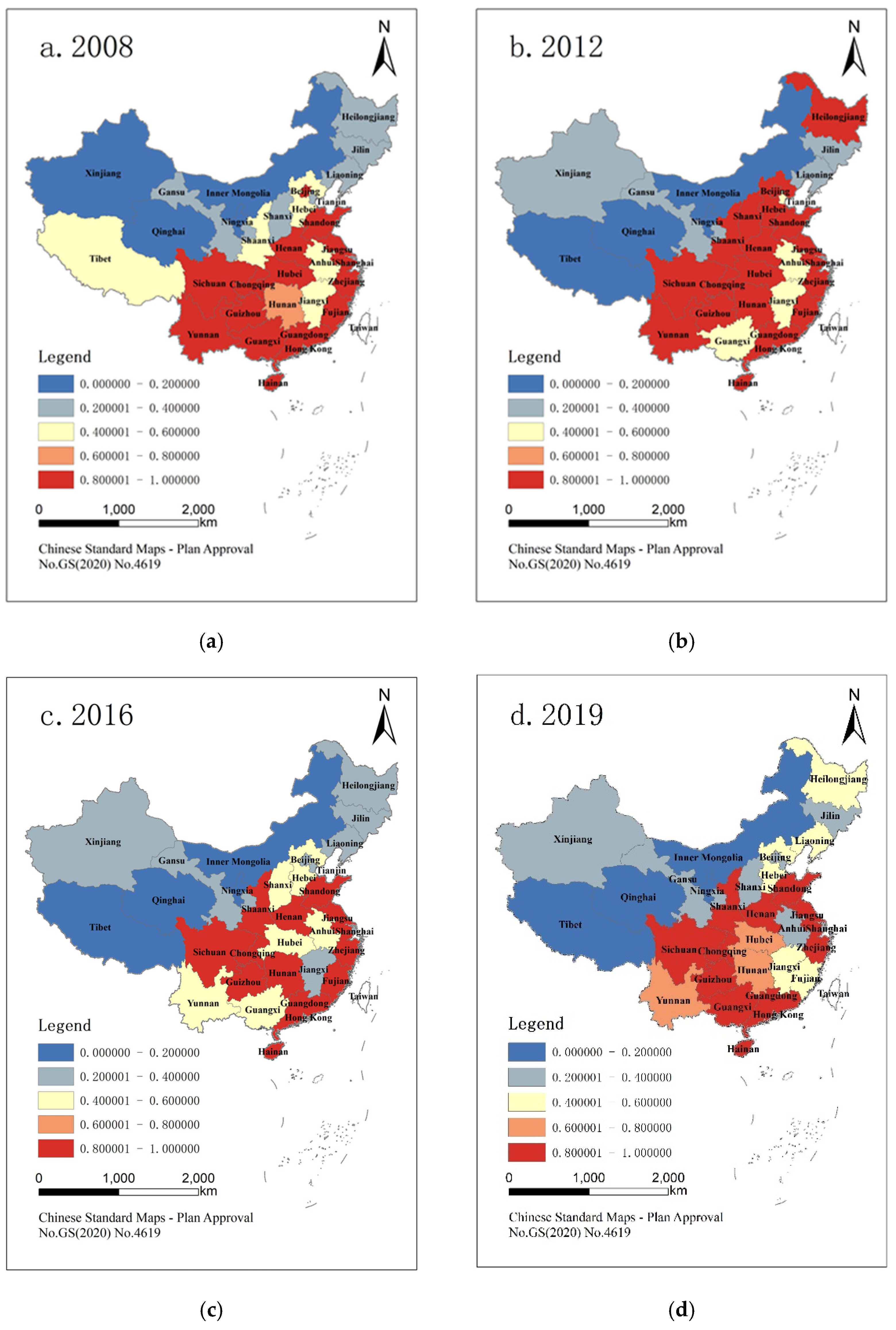
In order to analyze AWUE, this paper used ArcGIS 10.2 software to visualize the AWUE of each province (Figure 1). It can be seen from Figure 1 that the AWUE in each province varies greatly. Bounded by the Hu Line, the AWUE in most provinces to the north of the line was at low levels, while the AWUE in the provinces south of the line was mostly at high levels at the time of this study.

Figure 1.
Spatiotemporal evolution of China’s provincial agricultural water use efficiency (AWUE). The data in Figure 1 were calculated according to a slack-based data envelopment analysis (DEA) method, and data can be obtained from the corresponding author upon request (e-mail: gongguofang@2020.cqut.edu.cn). (a) China’s provincial AWUE in 2008; (b) China’s provincial AWUE in 2012; (c) China’s provincial AWUE in 2016; (d) China’s provincial AWUE in 2019.
In this paper, the DEA model was used to measure China’s AWUE between the years 2008 and 2019. According to the latest statistical system and classification standard issued by the China Bureau of Statistics, provinces in China were divided into eastern, central, and western regions, and AWUE was analyzed on this basis.
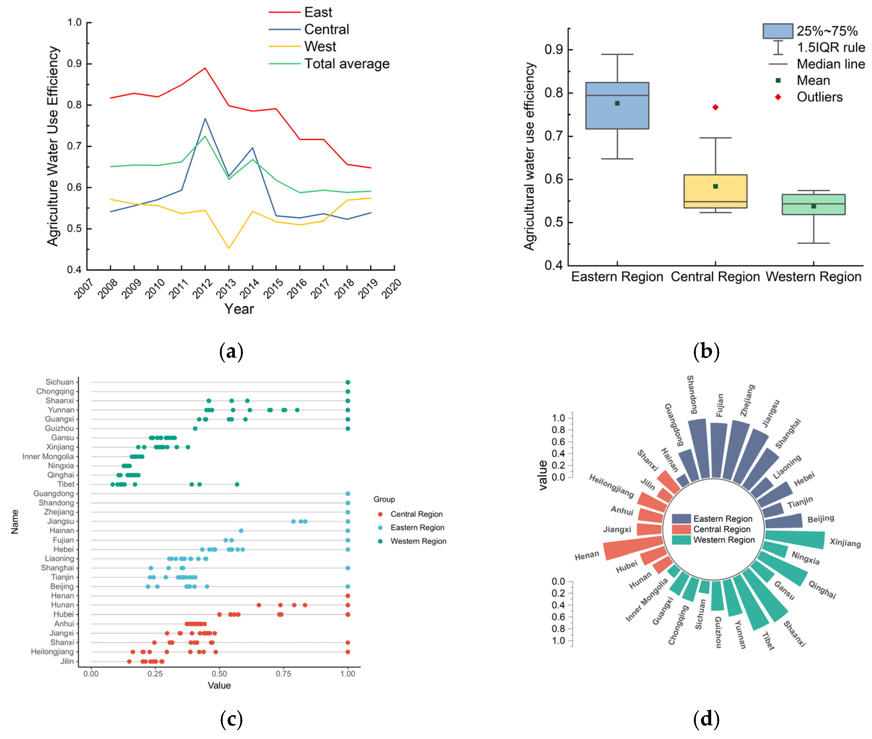
At the regional level (Figure 2a,b), there were obvious differences in AWUE in each region. The regional AWUE average from high to low was as follows: eastern, central, and western. From the perspective of temporal evolution, the overall AWUE in various regions has shown a fluctuating downward trend, and there is still great room for the improvement of AWUE. Specifically, from 2008 to 2019, AWUE in the eastern region was always ahead of the national average level, but showed a downward trend, and the efficiency value changed from 0.817 to 0.648. AWUE in the central region fluctuated greatly, and was lower than the national average in all years except for between 2012 and 2014. The overall level of AWUE in the western region was low, and the overall trend was to decline first and then rise.

Figure 2.
Agricultural water use efficiency (AWUE) zoning map: (a) average AWUE curves for the three regions and totals; (b) boxplots of the three regions; (c,d) distribution of AWUE at the provincial level.
At the provincial level (Figure 2c,d), AWUE in eastern regions such as Guangdong, Shandong, Zhejiang, and Jiangsu was high and relatively stable, while the AWUE in Beijing, Liaoning, and Tianjin was low, and had fluctuated greatly, leading to a downward trend in AWUE in eastern regions to a certain extent. In the central region, the efficiency in Henan, Hunan, and Hubei was high, and the efficiency in other provinces had fluctuated greatly. There have been significant differences among provinces in the western region, except for the efficiency values of Sichuan and Chongqing, which have been stable at 1. The efficiency values of other provinces have fluctuated greatly and have been relatively low, which is the reason why the AWUE in the western region has always been lower than the average national level.
4.2. Structural Characteristics of the Spatial Association Network
4.2.1. Overall Network Structure
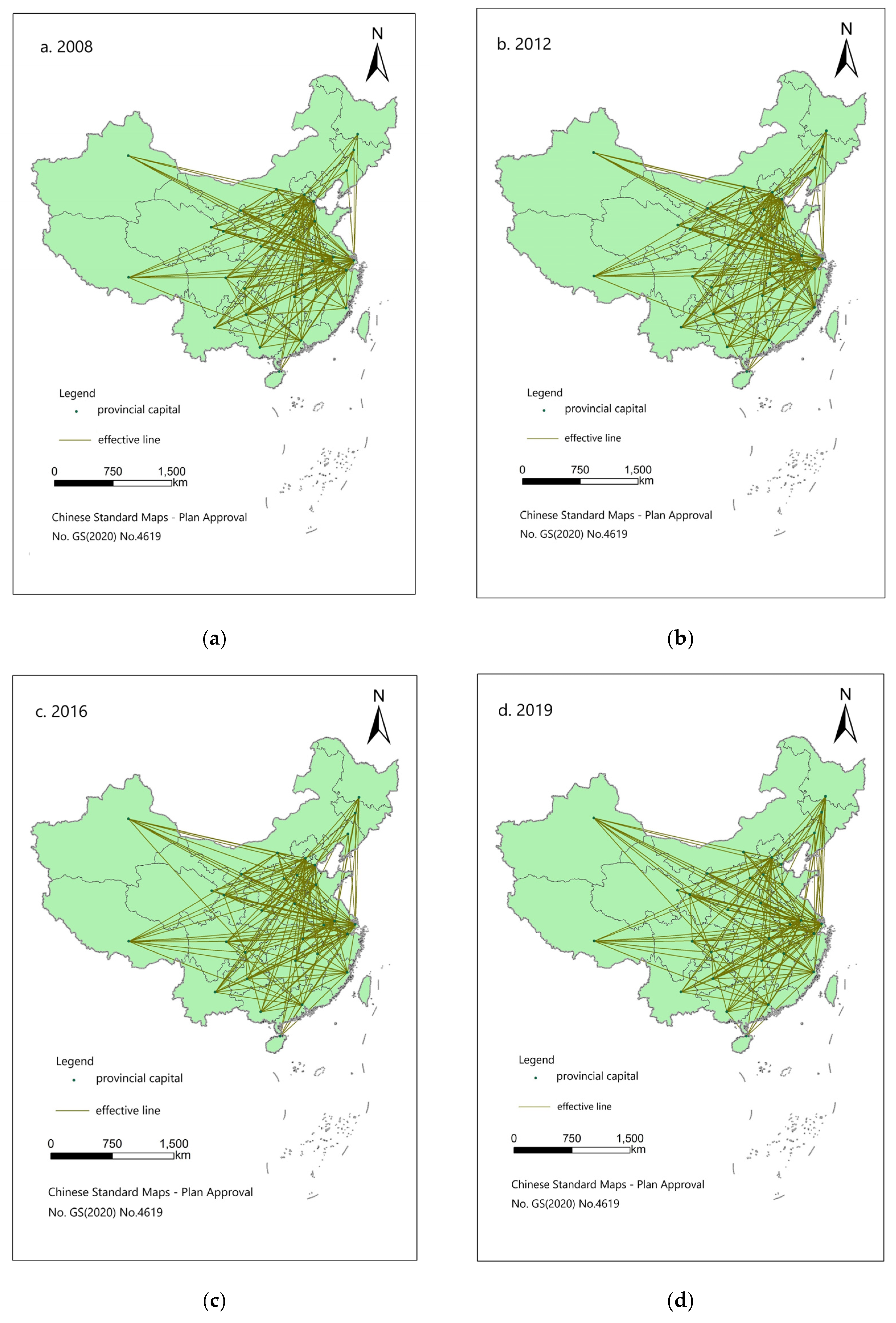
Based on the modified gravity model, the spatial association matrix was calculated. Subsequently, the spatial correlation network diagram of AWUE in China was drawn. Four years (2008, 2012, 2016, and 2019) were selected as representatives for horizontal comparison (Figure 3).
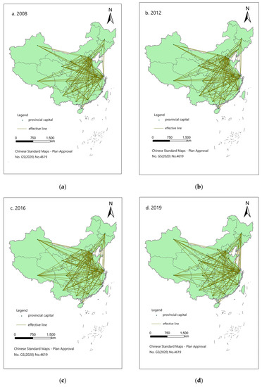
Figure 3.
Spatial correlation networks of China’s agricultural water use efficiency (AWUE): (a) spatial correlation networks of China’s AWUE in 2008; (b) spatial correlation networks of China’s AWUE in 2012; (c) spatial correlation networks of China’s AWUE in 2016; (d) spatial correlation networks of China’s AWUE in 2019.
Figure 3 shows that the spatial network structure of AWUE is closely related and complex. The entire spatial association network is connected, without isolated points. The network relationship number can be obtained through the spatial correlation matrix of China’s AWUE over time. The network density, connectedness, hierarchy, and efficiency were calculated according to Equations (1)–(4), respectively, so as to analyze the overall structural characteristics of China’s AWUE network. The calculation results are shown in Figure 4 and Figure 5.
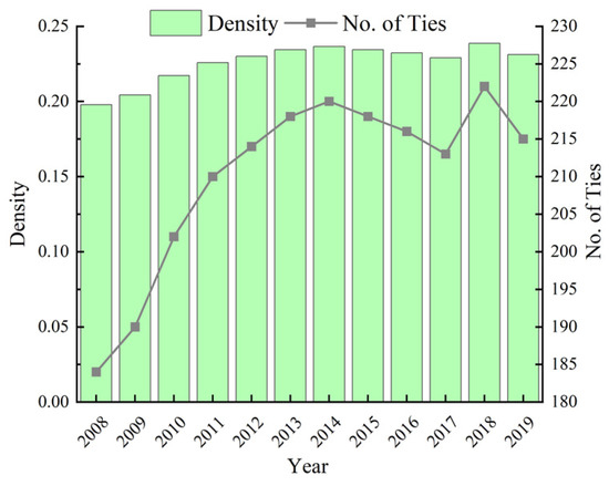
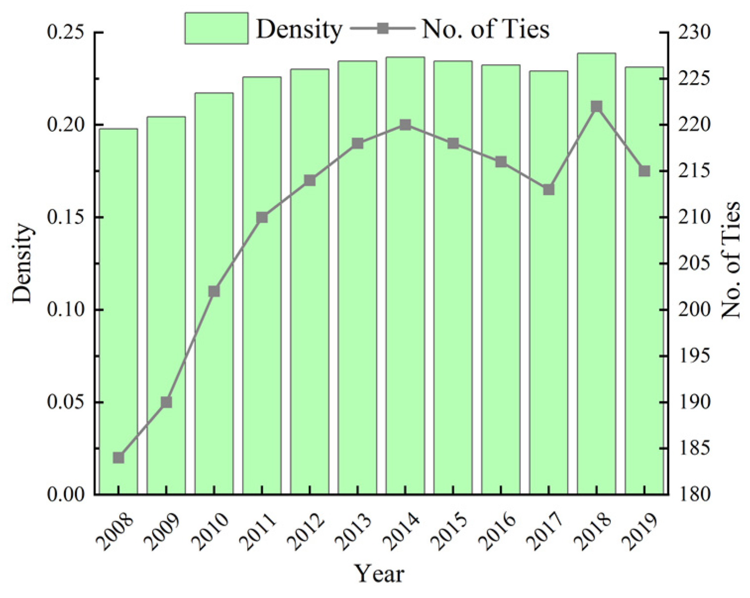
Figure 4.
The network density and relationships of province-level agricultural water use efficiency in China from 2008 to 2019.
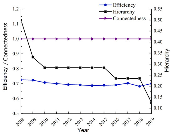
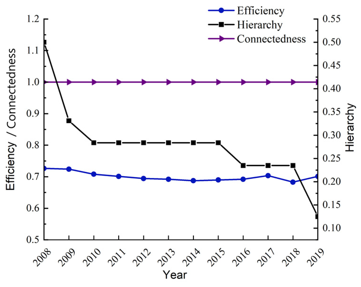
Figure 5.
Network connectedness, network hierarchy, and network efficiency of province-level agricultural water use efficiency in China from 2008 to 2019.
Figure 4 shows that the network density and number of network tie trends of AWUE in China between 2008 and 2019 were consistent, showing an overall growth; however, the overall range of change was small. The number of ties increased from 184 in 2008 to 215 in 2019—an increase of 16.85%. The network density increased from 0.1978 in 2008 to 0.2312 in 2019—an increase of 16.85%. However, the network density value was far lower than the medium level, and the number of network relationships was far lower than its maximum potential (930). During the study period, the network connectedness of AWUE in China was 1 (Figure 5). The network hierarchy shows an obvious downward trend, from 0.5000 in 2008 to 0.1250 in 2019, and the overall level of network efficiency was high, with an average of 0.7002.
4.2.2. Individual Network Characteristics
Degree centrality, closeness centrality, and betweenness centrality were used to analyze the status and spatial correlation characteristics of each province in the spatial correlation network of AWUE. The analysis showed that during the 2008 to 2019 period, provinces with higher centrality rankings did not change significantly, with Shanghai, Beijing, Jiangsu, and Zhejiang ranking higher in centrality. In order to ensure that the research results were more in line with the current situation, the data from 2019 were analyzed, because they were the latest available information.
- 1.
- Degree centrality
It can be seen from Table 2 that the average degree centrality in the spatial correlation network of AWUE in all provinces of China was 34.409, and the development of AWUE in all provinces was uneven. There were seven provinces whose degree centrality exceeded the average level: Shanghai, Jiangsu, Beijing, Zhejiang, Fujian, Hubei, and Gansu. Most of these provinces are located in the developed eastern areas, indicating that the eastern region is located in the center of the spatial correlation network structure of AWUE, and has a particularly large impact on the spatial distribution of AWUE. Shanghai had the highest degree centrality, indicating that Shanghai is at the core of the spatial correlation network of AWUE. This may be due to the fact that Shanghai has a developed economy, a developed transportation network, convenient contact with other provinces, good natural conditions, more advanced technology, and more funds and talent in agricultural development. With regard to out-degree centrality, there were 19 provinces that were higher than average, among which Gansu, Fujian, Shanghai, and Guangxi ranked highest, indicating that they had obvious spatial spillover effects. The out-degree centrality of all provinces in China was greater than 0, indicating that all provinces had radiation capacity. Regarding in-degree centrality, there were 10 provinces whose in-degree centrality was higher than average, indicating that these provinces received additional spillover relationships from other provinces. Shanghai had the highest in-degree centrality, indicating its strong agglomeration capacity. The in-degree centrality of Xinjiang and Tibet was 0, indicating that they did not have receiving relationships.
Table 2.
Centrality of the spatial association network of China’s provincial agricultural water use efficiency in 2019.
- 2.
- Closeness centrality
The average closeness centrality of AWUE in each province was 60.746, and the overall distribution was balanced, indicating that the AWUE of each province in the spatial correlation network is easily related to other provinces. The closeness centrality of Shanghai, Jiangsu, Beijing, Zhejiang, Fujian, Hubei, and Gansu was higher than the mean value, indicating that these provinces were the dominant players in the network and could quickly establish connections with other provinces. This may be due to the fact that these provinces are mostly located in the developed eastern regions, which have high water resource endowment, relatively developed agricultural technology, continuous optimization of their crop-planting structures, and rapid development of water-saving agriculture. Qinghai, Ningxia, Shaanxi, Hebei, Inner Mongolia, Anhui, and Guangdong ranked relatively low; most of these provinces are geographically remote, with less annual precipitation and underdeveloped economies; they are in a subordinate position in the spatial network of AWUE, have had less contact with other provinces, and their promotion effects when receiving other provinces were not significant.
- 3.
- Betweenness centrality
The average betweenness centrality of AWUE in each province was 4.690, and the overall distribution was not balanced. The betweenness centrality values of the provinces were quite different, indicating that there was a large difference in the control abilities between provinces. There were 12 provinces with above-average betweenness centrality, including Beijing, Chongqing, Fujian, Gansu, Shanghai, Guangdong, Jiangsu, Guangxi, Jiangxi, Hunan, Liaoning, and Guizhou. These provinces were in the key position of the spatial association network, and played an intermediary role; other provinces relied on these to a high extent. The betweenness centrality of Tibet, Qinghai, Jilin, and Xinjiang was 0; most of these provinces are located in northeastern and western China, with remote geographical locations, a lack of natural resources, lagging agricultural economic development, and poor industrial structures; therefore, these provinces have weak control abilities and strong dependence on other provinces.
4.2.3. Block Model Analysis
A block model was used to analyze the clustering characteristics and relationship overflow path of the spatial correlation network of AWUE in China. Using the CONCOR tool in the UCINET 6.0 software, with the maximum segmentation depth set to 2 and the concentration standard set to 0.2, the 31 provinces in the spatial correlation network of China’s AWUE were divided into 4 sections (Table 3): Plate I includes Beijing, Tianjin, Jiangsu, Zhejiang, and Shanghai; Plate II includes Guangdong, Hubei, and Fujian; Plate III includes Inner Mongolia, Jilin, Heilongjiang, Shaanxi, Liaoning, Hebei, Shandong, Ningxia, Shanxi, and Chongqing; and Plate IV includes Jiangxi, Hunan, Guangxi, Hainan, Henan, Guizhou, Yunnan, Tibet, Anhui, Gansu, Qinghai, Sichuan, and Xinjiang.
Table 3.
Spillover effect of spatial correlation plates of China’s provincial agricultural water use efficiency.
It can be seen from Table 3 that there were 215 relationships in the spatial correlation network of AWUE in China, including 26 internal relationships and 189 inter-plate relationships. This indicates that AWUE had spatial overflow between plates. The expected internal relationship proportions of the first sector were less than the actual internal relationship proportions. The sector received 102 related relationships from other plates, and sent 25 related relationships to other plates. The number of received relationships was significantly more than the number of sent relationships, meaning this sector belongs to the “net benefit” plate. The second plate received 31 contacts and sent 23 contacts. The number of relationships received from other plates was more than the number sent to other plates, and the number of external contacts was greater than the number of internal contacts; therefore, Plate II was a “bidirectional spillover” plate, and was affected by the spillover relationships of other plates while also having a spillover effect onto other plates. The actual internal relationship proportions of Plate III were lower than the expected internal relationship proportions. This plate had more relationships from receiving other plates and spilling over onto other plates; therefore, Plate III was the “broker” plate. The number of contacts sent by the fourth plate was significantly greater than the number received; thus, Plate IV was the “net spillover” plate. Most of the provinces in this plate were located in the central and western regions, with poor water resources and strong spatial spillover effects.
In order to further analyze the spatial correlations and conduction paths between plates, the density matrices between plates were calculated. Regarding the comparison of the plate density values with the spatial network density values of China’s AWUE in 2019, if they were greater than 0.2312, they were assigned a value of 1; if not, they were assigned a value of 0. After completion, the image matrix was obtained. The image matrix clearly shows the conduction paths between plates (Table 4). It can be seen from the density matrix that the internal network density of Plate I was 0.300, and that its density value was the highest among the four plates, indicating that there was a significant correlation within it. However, the internal network density of Plates II, III, and IV was lower, indicating that their internal correlations were smaller. It can be seen from the image matrix that only Plate I had a close internal spillover relationship, showing that the AWUE linkage of the provinces in the eastern developed regions was strong. The correlation coefficients of AWUE generated by Plates III and IV and affected by Plates I and II were much larger than those of Plates I and II affected by Plates III and IV. Therefore, Plates III and IV were more representative as “contributors” to the relationship between Plates I and II. This is due to the fact that the provinces in Plates I and II had a high level of economic development and high scientific and technological strength. Second, due to industrial structure, population size, geographical environment, and other reasons, the Yangtze River Delta, Pearl River Delta, and Beijing–Tianjin–Hebei regions also consumed many resources. These regions developed more secondary and tertiary industries. Plates III and IV carried out purchases of agricultural products, which led to pressure on AWUE in those plates. In addition, Plate III was serving Plate I, while Plate IV was serving Plate II, which may be related to geographical distance.
Table 4.
Density and image matrices of spatial plates for China’s provincial agricultural water use efficiency.
4.3. Factors Influencing the Spatial Association Network
4.3.1. Quadratic Assignment Procedure Correlation Analysis
In this paper, UCINET software was used to analyze the factors affecting AWUE’s spatial association network. Table 5 shows the results from 5000 random permutations that were selected. It can be seen from Table 5 that the correlation coefficients of geographical adjacency (GA), natural endowments (NE), technological level (TE), and farmers’ income (FI) all passed the 1% significance level test, and the proportion of tertiary and primary industries (PTP) and agricultural crop structure (ACS) both passed the 5% significance level test. This shows that these six factors have significantly affected the formation of AWUE’s spatial association network structure in China. The correlation coefficients of GA, TE, FI, and PTP were positive, indicating a positive correlation between these coefficients and AWUE’s spatial correlation. The correlation coefficients of NE and ACS were negative, indicating that there was a negative correlation between these coefficients and AWUE’s spatial correlation. The correlation coefficients of the difference between the proportion of grain production and meat production (PGM) and irrigation infrastructure (IF) were not significant, indicating that their effect on spatial correlation was not obvious.
Table 5.
Quadratic assignment procedure correlation analysis results of the spatial correlation matrix Y and its influencing factors.
4.3.2. Quadratic Assignment Procedure Regression Analysis
According to the results of the QAP correlation analysis, this study abandoned the two influencing factors of PGM and IF. In order to avoid multicollinearity between influencing factors, this paper used the QAP regression analysis to set the number of random replacements to 10,000 times, so as to explore the relationships between the remaining six factors and the spatial association network structure of AWUE. The regression results are shown in Table 6. The results show that the adjusted R2 was 0.256, indicating that the interpretation degree of the regression equation to the spatial association network structure of AWUE was 25.6%. GA, TE, FI, and NE all passed the significance test, indicating that they had a significant impact on the formation of the spatial correlation network.
Table 6.
Quadratic assignment procedure regression analysis results.
Specifically, the regression coefficient of GA passed the 1% significance level test, and was positive, indicating that GA played a significant role in promoting the formation of AWUE’s spatial correlation. This was due to the fact that the provinces with short geographical distance were more easily able to carry out resource and population flows, resulting in higher spatial correlations. The greater the spatial distance, the greater the difficulty of spatial spillover.
NE was significant at a level of 5%, and its regression coefficient was negative, indicating that precipitation was also a key factor in the formation of AWUE’s spatial correlation. The negative regression coefficient indicates that the narrowing of the water resource endowment gap was conducive to the formation of the AWUE spatial connections between provinces. This may be due to the fact that, with the development of the South-to-North Water Diversion Project in recent years, it has been easier for water resources to flow between the different provinces.
The regression coefficient of TE was significantly positive at 1%, implying that the widening of TE differences had a positive effect on the formation of spatial associations. This was due to the fact that the widening of TE differences exacerbated the disparities in the level of water resource use between provinces, promoted cross-regional cooperation, and strengthened spatial connections.
FI was significant at a level of 5%, and its regression coefficient was positive, indicating that FI played a significant role in promoting the formation of AWUE’s spatial correlation. The positive regression coefficient means that the greater the difference in FI among provinces, the greater the spatial relevance of AWUE. This was due to the fact that areas with higher FI were more likely to accept advanced agricultural technology development ideas and have the ability to adopt efficient water-saving technology and facilities, while areas with low FI were not. This led to the disparity in the levels of water resource utilization between provinces. In order to coordinate regional development, the Chinese government has encouraged farmers to communicate across regions and strengthen spatial connections.
The regression coefficients of PTP and ACS were not significant, indicating that they had no significant impact on the spatial correlations of AWUE, which may be because their industrial and crop structures were relatively stable.
5. Discussion
Unlike previous studies [12,18], this paper calculated AWUE and then analyzed the gaps between the regions from the results. This study aimed to explore the spatial relevance of China’s interprovincial AWUE from the perspective of its social network, and to determine the factors affecting the spatial correlation network. Not only were the overall and individual characteristics of the spatial correlation network analyzed, the influencing factors of the spatial correlation network were also explored.
First, this paper used the slack-based DEA method and ArcGIS visualization tool to find that the agricultural development in the eastern and central regions has not made effective progress between 2008 and 2019, while the agricultural development in the western region has been effectively developed. Then, using the modified gravity model, it was found that the interprovincial AWUE in China presents a complex spatial correlation network structure (Figure 1). These findings show that the improvement of AWUE needs to include regional collaborative governance measures in order to improve overall AWUE. This result is consistent with the new regionalism principle put forward by Ethier [53]—that is, the promotion of regional integration and coordinated development. In addition, although the AWUE in the developed eastern regions has been increasing slowly, it has been at a high level and at the core of the spatially correlated network. The eastern coastal provinces should play an exemplary role in promoting the development of the central and western provinces. The findings of Wang, et al. [24] were similar to those of this study.
Second, the network density and number of network tie trends of AWUE showed an increasing trend, but were far lower than the medium level, indicating that the spatial correlation of AWUE has become closer, and that there is significant room for improvement in China’s AWUE network (Figure 4). From the evolution of spatial correlation network efficiency (Figure 5), the spatial correlation network of AWUE in China has gradually been balanced, and cooperation and communication between provinces have been continuously strengthened. There were many redundant correlation coefficients in the network. There was also an obvious spatial overflow of multiple superpositions, and the spatial correlation network was relatively stable. In recent years, as the Chinese government has implemented a series of measures such as industrial structure optimization, large-scale water resource allocation activities, and agricultural water conservancy construction, the AWUE in various provinces has improved to varying degrees; this finding is consistent with the findings of Geng [54]. Therefore, more labor, technology, and funds need to be invested in agricultural development and agricultural water management.
Third, the differences in geographical adjacency, technological level, farmers’ income, and natural endowment had a significant impact on AWUE’s spatial association network. Wang, et al. [43] found that geographic adjacency is significantly related to the formation of spatial association networks; their finding was similar to the findings in this study. Therefore, in order to improve AWUE in China, it is necessary to continuously improve the level of regional technology and economic development, so as to achieve the simultaneous improvement of economic benefits, technology, and agricultural green benefits.
In summary, these findings provide a scientific theoretical basis for improving AWUE in China, and provide a theoretical basis for the Chinese government to formulate reasonable policies. Therefore, based on the above conclusions, the following policy recommendations can be made:
- (1)
- The government should fully understand the spatial correlation and network structure characteristics of AWUE, break through the barriers of regional factor flow, strengthen interprovincial cooperation, and improve the spatial allocation efficiency of wide-area spatial resources. The market plays a decisive role in resource allocation. The government should give full attention to the leading role of the market in regional coordinated development, create more favorable conditions for the cross-regional cooperative utilization of agricultural water resources, optimize spatial allocation, break the administrative barriers between regions, and promote the flow of various production factors between regions so as to obtain comparative benefits in national production activities;
- (2)
- Attention should be paid to the spatial differences in AWUE in China. There are large differences in AWUE across China, and the economic development, industrial structure, and technological stages of the eastern, central, and western regions have been at different levels. Therefore, each region should adapt to local conditions and formulate policies and strategies suitable for the sustainable development of water resources in the region. The government should also increase its support for the central and western regions, fully implement strategies such as “the development campaign of the western regions” and “the rise of the Central Plains”, decrease regional differences, and achieve a coordinated development of AWUE in different regions;
- (3)
- The government should implement the overall strategy of coordinated regional development and accelerate the construction of a new mechanism for coordinated regional development that is more effective. According to the research results, the eastern region has been at the core of China’s AWUE spatial correlation network. For example, Shanghai, Jiangsu, Zhejiang, Beijing, and other provinces can use their own economic and technological advantages to increase regional cooperation and exchange, play leading roles, and promote the improvement of AWUE in the central and western regions. The central region is a bridge connecting the eastern and western regions; therefore, the central region should establish the concept of regional coordinated development. For example, Shanxi, Hubei, and other places can improve the extent to which they communicate with the outside world, promote cooperation between the central region and other regions, and achieve a win–win situation. The western region, including Xinjiang, Tibet, and Qinghai, has accepted more spatial spillover relations; therefore, on the one hand, the western region actively uses the funds and technologies spilled from the east to promote the improvement of regional AWUE; on the other hand, it needs to improve its own development environment, accelerate the optimization and upgrading of its industrial structure, increase its investment in technology and education, and strive to improve AWUE;
- (4)
- Considering the driving factors of China’s AWUE spatial association network, the government should focus on strengthening interprovincial cooperation in the fields of economic and technological development. It is necessary to strengthen interprovincial cooperation in the fields of economy, technology, and transportation, improve the flow of production factors, decrease the gaps between provinces, and promote the development of the AWUE spatial correlation network between regions.
6. Conclusions
Based on the 2008 to 2019 interprovincial AWUE in China measured by the slack model, this paper used the modified gravity model to determine the spatial correlation matrix of interprovincial AWUE in China. Subsequently, SNA was used to reveal the characteristics of China’s interprovincial AWUE spatial correlation network. Finally, the QAP correlation and regression analysis methods were used to study the influencing factors of China’s interprovincial AWUE spatial correlation network. The conclusions are as follows:
- (1)
- The overall trend of AWUE in China has been fluctuating and declining, and there is still a significant amount of room for improvement when it comes to AWUE. There are obvious differences in AWUE in each region, and the regional averages of AWUE descend from high to low in the eastern region, the central region, and the western region;
- (2)
- The overall structure of AWUE’s spatial network is complex, balanced, and robust, and the members are closely connected. In terms of individual network characteristics, there are obvious differences in the statuses of provinces in the associated network. Eastern regions such as Shanghai, Beijing, Jiangsu, and Zhejiang have been at the center of the network, and have played an important role in the spatial correlation network. The centrality of western regions such as Xinjiang, Qinghai, Tibet, and Inner Mongolia has been relatively low, and they have been on the edge of the spatial correlation network, holding few links with other provinces. From the perspective of spatial agglomeration characteristics, the AWUE spatial association network can be divided into four plates. Most of the eastern provinces belong to the main inflow areas, and most of the central and western provinces belong to the main outflow areas;
- (3)
- The results of the QAP correlation and regression analysis showed that the expansion of GA, TE, and FI and the reduction of NE would significantly promote the development of spatial AWUE associations.
Author Contributions
Conceptualization, G.Y.; data curation, Q.G. and G.G.; methodology, G.Y.; resources, Q.G.; writing—review and editing, G.G. and G.Y.; visualization, Q.G.; project administration, G.Y.; funding acquisition, G.Y. All authors have read and agreed to the published version of the manuscript.
Funding
This research was funded by the Science and Technology Research Program of Chongqing Municipal Education Commission (Grant No. KJQN202101122 and No. KJQN201904002).
Institutional Review Board Statement
Not applicable.
Informed Consent Statement
Not applicable.
Data Availability Statement
The data used to support the findings of this study are available from the corresponding author upon request (e-mail: alexandrakung@163.com).
Acknowledgments
The authors would like to thank the anonymous reviewers for their valuable comments on drafts of this paper.
Conflicts of Interest
The authors declare no conflict of interest.
References
- UN-Water. The United Nations World Water Development Report 2021: Valuing Water; UNESCO: Paris, France, 2021; pp. 9–10.
- UN-Water. The United Nations World Water Development Report 2018: Nature-based Solutions for Water; UNESCO: Paris, France, 2018; pp. 22–23.
- FAO. The State of the World’s Land and Water Resources for Food and Agriculture: Managing Systems at Risk; Earthscan: London, UK, 2011. [Google Scholar]
- Fan, J.; Wang, J.; Zhang, X.; Kong, L.; Song, Q. Exploring the changes and driving forces of water footprints in China from 2002 to 2012: A perspective of final demand. Sci. Total Environ. 2019, 650, 1101–1111. [Google Scholar] [CrossRef] [PubMed]
- D’Odorico, P.; Chiarelli, D.D.; Rosa, L.; Bini, A.; Zilberman, D.; Rulli, M.C. The global value of water in agriculture. Proc. Natl. Acad. Sci. 2020, 117, 21985. [Google Scholar] [CrossRef]
- Fuentes, E.; Arce, L.; Salom, J. A review of domestic hot water consumption profiles for application in systems and buildings energy performance analysis. Renew. Sust. Energ. Rev. 2018, 81, 1530–1547. [Google Scholar] [CrossRef]
- Jia, Z.; Cai, Y.; Chen, Y.; Zeng, W. Regionalization of water environmental carrying capacity for supporting the sustainable water resources management and development in China. Resour. Conserv. Recycl. 2018, 134, 282–293. [Google Scholar] [CrossRef]
- Zhao, Z.-Y.; Zuo, J.; Zillante, G. Transformation of water resource management: A case study of the South-to-North Water Diversion project. J. Clean. Prod. 2017, 163, 136–145. [Google Scholar] [CrossRef]
- Farrell, M.J. The Measurement of Productive Efficiency. J. R Stat. Soc. Ser. A 1957, 120, 253–281. [Google Scholar] [CrossRef]
- Wallach, B. International Commission on Irrigation And Drainage. Prof. Geogr. 1984, 36, 490–491. [Google Scholar] [CrossRef]
- Van Halsema, G.E.; Vincent, L. Efficiency and productivity terms for water management: A matter of contextual relativism versus general absolutism. Agric. Water Manag. 2012, 108, 9–15. [Google Scholar] [CrossRef]
- Zhang, F.; Xiao, Y.; Gao, L.; Ma, D.; Su, R.; Yang, Q. How agricultural water use efficiency varies in China—A spatial-temporal analysis considering unexpected outputs. Agric. Water Manag. 2022, 260, 107297. [Google Scholar] [CrossRef]
- Benedetti, I.; Branca, G.; Zucaro, R. Evaluating input use efficiency in agriculture through a stochastic frontier production: An application on a case study in Apulia (Italy). J. Clean. Prod. 2019, 236, 117609. [Google Scholar] [CrossRef]
- Tu, V.H.; Can, N.D.; Takahashi, Y.; Yabe, M. Water Use Efficiency in Rice Production: Implications for Climate Change Adaptation in the Vietnamese Mekong Delta. Proc. Integr. Optim. 2018, 2, 221–238. [Google Scholar] [CrossRef]
- Gautam, T.K.; Paudel, K.P.; Guidry, K.M. An Evaluation of Irrigation Water Use Efficiency in Crop Production Using a Data Envelopment Analysis Approach: A Case of Louisiana, USA. Water 2020, 12, 3193. [Google Scholar] [CrossRef]
- Geng, Q.; Ren, Q.; Nolan, R.H.; Wu, P.; Yu, Q. Assessing China’s agricultural water use efficiency in a green-blue water perspective: A study based on data envelopment analysis. Ecol. Indic. 2019, 96, 329–335. [Google Scholar] [CrossRef]
- Song, M.; Wang, R.; Zeng, X. Water resources utilization efficiency and influence factors under environmental restrictions. J. Clean. Prod. 2018, 184, 611–621. [Google Scholar] [CrossRef]
- Wang, G.; Chen, J.; Wu, F.; Li, Z. An integrated analysis of agricultural water-use efficiency: A case study in the Heihe River Basin in Northwest China. Phys. Chem. Earth 2015, 89–90, 3–9. [Google Scholar] [CrossRef]
- Dhehibi, B.; Lachaal, L.; Elloumi, M.; Messaoud, E.B. Measuring irrigation water use efficiency using stochastic production frontier: An application on citrus producing farms in Tunisia. Afr. J. Agric. Resour. E 2007, 1, 1–15. [Google Scholar] [CrossRef]
- Lu, X.; Xu, C. The difference and convergence of total factor productivity of inter-provincial water resources in China based on three- stage DEA-Malmquist index model. Sustain. Comput-Infor. 2019, 22, 75–83. [Google Scholar] [CrossRef]
- Garcia y Garcia, A.; Guerra, L.C.; Hoogenboom, G. Water use and water use efficiency of sweet corn under different weather conditions and soil moisture regimes. Agric. Water Manag. 2009, 96, 1369–1376. [Google Scholar] [CrossRef]
- Sadras, V.; Rodriguez, D. The limit to wheat water-use efficiency in eastern Australia. II. Influence of rainfall patterns. Aust. J. Agric. Res. 2007, 58, 657–669. [Google Scholar] [CrossRef]
- Song, J.; Chen, X. Eco-efficiency of grain production in China based on water footprints: A stochastic frontier approach. J. Clean. Prod. 2019, 236, 117685. [Google Scholar] [CrossRef]
- Wang, F.; Yu, C.; Xiong, L.; Chang, Y. How can agricultural water use efficiency be promoted in China? A spatial-temporal analysis. Resour. Conserv. Recycl. 2019, 145, 411–418. [Google Scholar] [CrossRef]
- Deng, X.; Shan, L.; Zhang, H.; Turner, N.C. Improving agricultural water use efficiency in arid and semiarid areas of China. Agric. Water Manag. 2006, 80, 23–40. [Google Scholar] [CrossRef]
- Kang, S.; Hao, X.; Du, T.; Tong, L.; Su, X.; Lu, H.; Li, X.; Huo, Z.; Li, S.; Ding, R. Improving agricultural water productivity to ensure food security in China under changing environment: From research to practice. Agric. Water Manag. 2017, 179, 5–17. [Google Scholar] [CrossRef]
- Hong, N.B.; Yabe, M. Improvement in irrigation water use efficiency: A strategy for climate change adaptation and sustainable development of Vietnamese tea production. Environ. Dev. Sustain. 2017, 19, 1247–1263. [Google Scholar] [CrossRef]
- Wang, X. Irrigation Water Use Efficiency of Farmers and Its Determinants: Evidence from a Survey in Northwestern China. Agric. Sci. China. 2010, 9, 1326–1337. [Google Scholar] [CrossRef]
- Lu, W.; Liu, W.; Hou, M.; Deng, Y.; Deng, Y.; Zhou, B.; Zhao, K. Spatial–Temporal Evolution Characteristics and Influencing Factors of Agricultural Water Use Efficiency in Northwest China—Based on a Super-DEA Model and a Spatial Panel Econometric Model. Water 2021, 13, 632. [Google Scholar] [CrossRef]
- Bai, C.; Zhou, L.; Xia, M.; Feng, C. Analysis of the spatial association network structure of China’s transportation carbon emissions and its driving factors. J. Environ. Manag. 2020, 253, 109765. [Google Scholar] [CrossRef]
- Chen, Z.; Sarkar, A.; Rahman, A.; Li, X.; Xia, X. Exploring the drivers of green agricultural development (GAD) in China: A spatial association network structure approaches. Land Use Policy 2022, 112, 105827. [Google Scholar] [CrossRef]
- Wang, Z.; Liu, Q.; Xu, J.; Fujiki, Y. Evolution characteristics of the spatial network structure of tourism efficiency in China: A province-level analysis. J. Destin. Mark. Manag. 2020, 18, 100509. [Google Scholar] [CrossRef]
- Huang, C.; Yin, K.; Liu, Z.; Cao, T. Spatial and Temporal Differences in the Green Efficiency of Water Resources in the Yangtze River Economic Belt and Their Influencing Factors. Int. J. Environ. Res. Public Health 2021, 18, 3101. [Google Scholar] [CrossRef]
- Xu, X.; Zhao, Y.; Wei, Q. Study on Spatial Network Structure of China’s Provincial Water Footprint Intensity and Its Cause of Formation. Stat. Decis. 2019, 35, 84–88. [Google Scholar] [CrossRef]
- ArcGIS. Available online: http://www.esri.com/software/arcgis (accessed on 19 February 2022).
- Yang, G.; Zhang, F.; Zhang, F.; Ma, D.; Gao, L.; Chen, Y.; Luo, Y.; Yang, Q. Spatiotemporal changes in efficiency and influencing factors of China’s industrial carbon emissions. Environ. Sci. Pollut. Res. 2021, 28, 36288–36302. [Google Scholar] [CrossRef] [PubMed]
- Tone, K. A slacks-based measure of efficiency in data envelopment analysis. Eur. J. Oper. Res. 2001, 130, 498–509. [Google Scholar] [CrossRef] [Green Version]
- Cooper, W.W.; Seiford, L.M.; Tone, K. Data Envelopment Analysis: A Comprehensive Text with Models, Applications, References and DEA-Solver Software; Springer: Berlin/Heidelberg, Germany, 2007; Volume 2. [Google Scholar]
- Sun, H.; Geng, Y.; Hu, L.; Shi, L.; Xu, T. Measuring China’s new energy vehicle patents: A social network analysis approach. Energy 2018, 153, 685–693. [Google Scholar] [CrossRef]
- Huang, M.; Wang, Z.; Chen, T. Analysis on the theory and practice of industrial symbiosis based on bibliometrics and social network analysis. J. Clean. Prod. 2019, 213, 956–967. [Google Scholar] [CrossRef]
- Wasserman, S.; Faust, K. Social Network Analysis: Methods and Applications; Cambridge University Press: Cambridge, UK, 1994. [Google Scholar]
- He, Y.; Wei, Z.; Liu, G.; Zhou, P. Spatial network analysis of carbon emissions from the electricity sector in China. J. Clean. Prod. 2020, 262, 121193. [Google Scholar] [CrossRef]
- Wang, Y.; Chen, Z.; Wang, X.; Hou, M.; Wei, F. Research on the Spatial Network Structure and Influencing Factors of the Allocation Efficiency of Agricultural Science and Technology Resources in China. Agriculture 2021, 11, 1170. [Google Scholar] [CrossRef]
- Su, Y.; Yu, Y. Spatial association effect of regional pollution control. J. Clean. Prod. 2019, 213, 540–552. [Google Scholar] [CrossRef]
- Carrington, P.J.; Scott, J.; Wasserman, S. Models and Methods in Social Network Analysis; Cambridge University Press: Cambridge, UK, 2005; Volume 28. [Google Scholar]
- Gan, C.; Voda, M.; Wang, K.; Chen, L.; Ye, J. Spatial network structure of the tourism economy in urban agglomeration: A social network analysis. J. Hsop. Tour. Manag. 2021, 47, 124–133. [Google Scholar] [CrossRef]
- Kaur, L.; Kaur, A.; Brar, A.S. Water use efficiency of green gram (Vigna radiata L.) impacted by paddy straw mulch and irrigation regimes in north-western India. Agric. Water Manag. 2021, 258, 107184. [Google Scholar] [CrossRef]
- Zhang, Q.; Sun, P.; Singh, V.P.; Chen, X. Spatial-temporal precipitation changes (1956–2000) and their implications for agriculture in China. Glob. Planet. Change 2012, 82–83, 86–95. [Google Scholar] [CrossRef]
- Mu, L.; Fang, L.; Wang, H.; Chen, L.; Yang, Y.; Qu, X.J.; Wang, C.Y.; Yuan, Y.; Wang, S.B.; Wang, Y.N. Exploring Northwest China’s agricultural water-saving strategy: Analysis of water use efficiency based on an SE-DEA model conducted in Xi’an, Shaanxi Province. Water Sci. Technol. 2016, 74, 1106–1115. [Google Scholar] [CrossRef] [PubMed]
- Liu, Y.; Hu, X.; Zhang, Q.; Zheng, M. Improving Agricultural Water Use Efficiency: A Quantitative Study of Zhangye City Using the Static CGE Model with a CES Water−Land Resources Account. Sustainability 2017, 9, 308. [Google Scholar] [CrossRef] [Green Version]
- Sun, C.; Han, Q.; Zheng, D. The spatial correlation of the provincial grey water footprint and its loading coefficient in China. Acta. Ecol. Sin. 2016, 36, 86–97. [Google Scholar] [CrossRef]
- Sun, C.Z.; Zhao, L.S. Water Resources Utilization Environmental Efficiency Measurement and Its Spatial Correlation Characteristics Analysis under the Environmental Regulation Background. Econ. Geogr. 2013, 33, 26–32. [Google Scholar]
- Ethier, W.J. The new regionalism. Econ. J. 1998, 108, 1149–1161. [Google Scholar] [CrossRef]
- Geng, X. On the regional differences in agricultural water use efficiency in China and their convergence. Int. J. Des. Nat. Ecodyn. 2020, 15, 189–196. [Google Scholar] [CrossRef]
Publisher’s Note: MDPI stays neutral with regard to jurisdictional claims in published maps and institutional affiliations. |
© 2022 by the authors. Licensee MDPI, Basel, Switzerland. This article is an open access article distributed under the terms and conditions of the Creative Commons Attribution (CC BY) license (https://creativecommons.org/licenses/by/4.0/).