Ecological Quality Response to Multi-Scenario Land-Use Changes in the Heihe River Basin

Abstract

To investigate the spatial-temporal effects of land-use changes on ecological quality and future trends, an integrated framework combining the Dyna-CLUE model and the remote sensing ecological index (RSEI) was developed. Land-use changes from 2000 to 2035 were simulated and projected under the current trend scenario (CTS), economic development scenario (EDS) and ecological protection scenario (EPS) in the Heihe River Basin, while the RSEI was predicted using the elastic net regression (machine learning method); finally, the predicted results were synthesized and analyzed. The results showed that forest, grassland and water were positively correlated with ecological quality, with the green space coverage under the CTS, EPS and EDS accounting for 34.15%, 70.65% and 34.72% of the total transferred land area, respectively. The increase in the area of build-up land and unutilized land was detrimental to ecological quality, with the area of building land in the EDS being 1.75 times larger than in the year 2000. The EDS contributes to the sustainable development of the upstream area and the EPS is more conducive to the midstream and downstream areas by limiting the expansion of build-up land and by developing unutilized land in a limited way to increase the area of green space after reconciling economic conditions. Projection results promote the rational allocation of various land-use types in the future (semi) arid region, such as artificial forestation, unutilized land development and restriction of urban expansion, and also lay the foundation for the formulation of policies such as water allocation and ecological protection to facilitate the sustainable development of regional society, economy and ecology.

1. Introduction

Rapid socio-economic development driven by the coaction of climate change and human activities has caused significant changes in land use/cover and ecological quality [1]. The fast-growing population, urbanization and farmland area have seriously threatened the co-development of water, ecosystem and socio-economy, such as soil pollution, carbon emissions and biodiversity loss [2], especially in (semi) arid regions [3]. Therefore, identifying the co-impacts of climate change and human intervention on ecological environment is crucial for co-development of the human environment.

Land-use changes have a significant impact on global challenges such as food security, climate change and biodiversity loss [4]. In the Brazilian Amazon, the expansion of farmland for soy production through deforestation [5,6] and the reduction of forest land for larger reservoirs and roads to encourage agricultural and entrepreneurial activities have led to the loss of biodiversity and increased forest degradation [7,8]. The coastal area around New Jiangwan Town in Shanghai, China, has decreased wetland and shrubland areas for urban expansion, with a corresponding decrease in bird biodiversity [9]. Reduced forest cover, increased forest patchiness and loss of river flow have been caused by oil exploitation and hydroelectric power plant operation in the Ecuadorian Amazon [10]. Understanding land-use changes under the influence of multiple economic, social and natural factors is the basis for improving ecological quality. In recent decades, various prediction models for land-use changes have been developed, and the most commonly used include the CA–Markov model and the Dyna-CLUE model. The CA–Markov model was developed to predict land-use changes under the influence of driving factors and historical trends to promote land conservation and rational land use [11,12]. It is mainly used for the prediction of land-use changes in a specific region [13,14], such as urban change trends and urban forecasting [15,16]. The Dyna-CLUE model is a framework for simulating land-use conversions that balances top–down location suitability with bottom–up land-use demand [17,18,19]. The model is used for prediction in various land-use studies, such as groundwater vulnerability assessment [20], future development assessments of agricultural lands [19,21] and change and prediction of forests or specific species of plants [22,23]. The logistic regression-based Dyna-CLUE model, which takes into account neighborhood effects, has a significant advantage in capturing land-use-change trends with more discrete distributions [24].

Remote sensing is a strong, time-continuous and highly spatially expressive tool for assessing ecological quality. The global ecosystem stability framework based on the normalized vegetation index has been used to assess ecosystem stability [25]. The remote sensing ecological index (RSEI) was used to evaluate the ecological quality of the region, taking Fuzhou, China, as an example, and was later widely applied [26,27]. For example, it was used to analyze the impact of impervious surfaces on the ecological status of the area, then assess the ecological status of the Xiongan New Area in Hebei, China [28], to detect spatial and temporal changes in ecological quality under climate and anthropogenic disturbances in basins [29,30] and to evaluate the ecological environment of mining areas and quantify the impact of land use on the ecological environment through RSEI [31].

The impacts of land-use changes on ecological quality have been increasingly emphasized, and existing studies include the relationship between past land-use changes and ecological quality and the impact of a particular land-use type on ecological quality. For example, a study conducted a spatial autocorrelation analysis and semi-variance analysis of RSEI values in Fuzhou City, Fujian Province, southeastern China, to evaluate the local ecological quality by quantifying the heterogeneity of the spatial distribution of the RSEI [32], and a combined approach integrating the random forest algorithm and RSEI was used to assess the ecological quality of Beijing [33]; the relationship between nighttime lighting data and the RSEI in the Yanqi Basin, a typical arid region of Xinjiang, China, revealed that the shift in the location of urbanized areas led to ecological degradation [34]. The effects on ecological quality of a single type of land-use change have been extensively studied, but ecological quality under the combined effects of multiple types of land-use changes requires continued research. Several existing policies have improved the relationship between land use and ecological quality, with the Yangtze River Basin in China showing an increase in wetland and forestland area from 2000–2018 due to the implementation of lake and wildlife habitat protection measures, benefiting biodiversity conservation and ecological sustainability [35]. The development of underutilized land into woodland, grassland and urban land in Jiayuguan City, China, is conducive to urbanization and oasis city completion [36]. Socio-economic restructuring and rural spatial adjustment in Yan’an City, China, have reduced the dependence of agricultural areas on resources and the environment and improved the man–land relationship [37]. The prediction of future ecological quality under the interaction of multiple land types and its guidance for policy are the emphasis of continued research.

The Heihe River Basin (HRB), the second largest inland river basin in northwestern China, experienced water shortages and environmental deterioration in the 1980s [38,39]. Since 2000, the ecological environment in the central and western parts of the HRB has been gradually restored under the influence of policies such as water diversion of the Heihe River and returning farmland to forest and grass [24]. However, economic development in the region is still dominant and land resources are over-exploited; the problems of sustainable development and ecological management cannot be ignored [40,41,42]. Therefore, the HRB, which is located in (semi) arid regions, was selected as the study area to investigate the ecological quality response to land-use changes.

Based on previous work, the effects of single land types such as over-cultivation of agricultural land, unreasonable water allocation or urban expansion on ecological quality that already exist have been extensively studied, but how multiple land-type changes jointly affect the development of ecological quality and how quantitative predictions of future land-use changes and ecological quality guide land allocation and ecological protection policies have not been well addressed. Therefore, in this study, a combination framework for predicting land-use changes and ecological quality is proposed by integrating remote sensing, land-use modeling and scenario analysis methods; the prediction results can be used as a basis for improving or formulating corresponding land allocation and ecological conservation policies. In this framework, a land-use model (Dyna-CLUE) as a multiple scenario prediction tool is applied to simulate and predict the interconversion between different land types, the RSEI and elastic network regression methods are used to evaluate and predict ecological quality and the framework integrates the results of land-use changes and ecological quality predictions for evaluation and analysis. In the scenario analysis, we take into account that social, economic and ecological development should be coordinated and sustainable, and the “Outline of the 14th Five-Year Plan (2021–2025) for National Economic and Social Development and Vision 2035 of the People’s Republic of China” as a policy driving factor is considered in the land transformation rules.

2. Materials and Methods

2.1. Study Area

This study was conducted in the Heihe River Basin (37°50′–42°40′ N, 98°–102° E) in northwestern China, total area of which is 1.43 × 10⁵ km² [43] (Figure 1). The Heihe River originates from Qilian Mountain of the upstream area, through a midstream oasis and terminates to Juyan lake in downstream area, the length of the main stream of which is 928 km. The average elevation of the upstream area is above 4000 m, with low temperature and relatively high precipitation of 250–500 mm. The midstream elevation is below 2000 m, with a large temperature difference, annual average temperature of 7 °C and precipitation between 110–370 mm. The downstream elevation is between 980–1200 m, arid and with long light hours, the average annual precipitation is 47 mm, and the evaporation is 2300 mm [39]. Land-use changes affect the ecological quality within the basin, and water as a land type is influenced by several factors. Climate warming, human activities (agricultural water use, surface water diversions and groundwater extraction [44]) and others have adversely affected water resources [45].

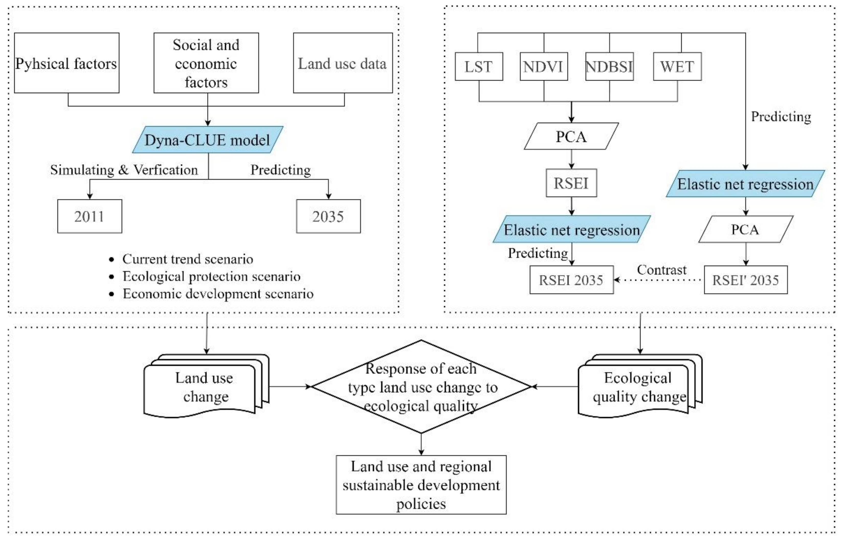
2.2. An Integration Framework for Predicting Land Use and Ecological Quality

An integration framework was developed to predict the RSEI used to express ecological quality and to project land-use changes under multiple scenarios, followed by an integrated analysis of the predictions (Figure 2). This framework consists of three components: (1) establishing the relationship between multiple drivers and each land type using the Dyna-CLUE model, then simulating and predicting land-use changes under multiple scenarios; (2) predicting future RSEI using the elastic network regression method (machine learning method) based on the calculated and processed existing RSEI data; (3) analyzing the distribution of RSEI values in different land-use types under different land-use scenarios, discussing the classification of land management and ecological protection policies in each region based on the analysis results and providing corresponding guidance. The first and second components of the framework are used for the prediction of land-use changes and RSEI, and the third component is used to integrate and analyze the results of the two components of the prediction and give policy recommendations.

2.3. Data

The data used in land-use model include land-use data and driver data, which are listed in

Table 1. List of base data and driving factors data in Dyna-CLUE modeling.

Data Type	Modeling Input Raster Data	Resolution	Data Sources
Base data	Land use data2000	-	National Tibetan Plateau Third Pole Environment Data Center (https://data.tpdc.ac.cn/en/data/320690e1-f8aa-4c51-a189-4c82f7e64b39/ (accessed on 7 July 2020)) [46,47]
	Land use data2011	-	National Tibetan Plateau Third Pole Environment Data Center (https://data.tpdc.ac.cn/en/data/b7ec37e6-339d-4777-80d3-bab18e6b7519/ (accessed on 7 July 2020)) [47,48]
Natural factors	DEM	1 km	National Tibetan Plateau Third Pole Environment Data Center (https://data.tpdc.ac.cn/en/data/d6776cbb-7bdc-4838-b361-389f43e241e1/ (accessed on 9 September 2020)) [49]
	Slope	1 km	National Tibetan Plateau Third Pole Environment Data Center (https://data.tpdc.ac.cn/en/data/d6776cbb-7bdc-4838-b361-389f43e241e1/ (accessed on 9 September 2020))
	Temperature	500 m	National Tibetan Plateau Third Pole Environment Data Center (https://data.tpdc.ac.cn/en/data/54d6c2f2-e499-456e-88ed-f044ea034c3c/ (accessed on 2 March 2021)) [50,51]
	Precipitation	500 m	National Tibetan Plateau Third Pole Environment Data Center (https://data.tpdc.ac.cn/en/data/8c00784a-f02a-49a3-b611-578cc62b0ede/ (accessed on 2 March 2021)) [52]
	Distance to river	-	National Tibetan Plateau Third Pole Environment Data Center (https://data.tpdc.ac.cn/en/data/7e10801a-7f23-4760-8b74-a284dabf78a0/ (accessed on 7 January 2021)) [53,54]
Economic factors	GDP	-	National Tibetan Plateau Third Pole Environment Data Center (https://data.tpdc.ac.cn/en/data/b18a2fb8-95fe-4ac4-b788-be88c0b6ec4a/ (accessed on 2 March 2021)) [55]
Social factors	Distance to highway	-	National Tibetan Plateau Third Pole Environment Data Center (https://data.tpdc.ac.cn/en/data/2cbd15cf-0591-41f2-a8d7-c4b8a232337c/ (accessed on 2 March 2021)) [54,56]
	Distance to road	-	National Tibetan Plateau Third Pole Environment Data Center (https://data.tpdc.ac.cn/en/data/2cbd15cf-0591-41f2-a8d7-c4b8a232337c/ (accessed on 2 March 2021))
	Distance to settlements	-	National Tibetan Plateau Third Pole Environment Data Center (https://data.tpdc.ac.cn/en/data/37bb0731-48fe-429b-8f09-6cc8dbac1f03/ (accessed on 2 March 2021)) [54,57]
	Population	1 km	National Tibetan Plateau Third Pole Environment Data Center (https://data.tpdc.ac.cn/en/data/032a5c57-df08-42ab-954e-218ef71cc28b/ (accessed on 21 September 2020)) [58,59]

. Thereinto, the six major land classifications (farmland, forest, grassland, water, build-up land and unutilized land) are taken into account in land-use datasets. The projection coordinates used in this study are WGS 1984 Albers and the spatial resolution is 1 km.

The driving factors include natural factors, social factors and economic factors. Among the natural factors, except for elevation and slope, which govern the plant growth environment, rainfall and temperature have a great impact on land-use changes in arid areas, making precipitation, temperature and distance to rivers the drivers [60,61,62]. An increase in the intensity of human activities (population increase, GDP, etc.) will directly reinforce water conflicts among water-using units in the basin, causing higher water stress; therefore, socio-economic factors such as population, roads and GDP are used as drivers.

The remote sensing images were used to calculate four indicators of heat, dryness, wetness and greenness from 2000 to 2020, and then the RSEI with a spatial resolution of 1 km was synthesized. Google Earth Engine (GEE, https://earthengine.google.com/ (accessed on 10 November 2021)) platform was used to calculate the annual means of the four indices by using the MODIS multi-temporal daily LST product (MOD11A1), the MODIS 16-day synthetic NDVI product (MOD13A2) and the daily surface reflectance combination (MOD09GA: sur_refl_b01 ~sur_refl_b07) were calculated annually for the four indices and then reprojected, resampled, masked and normalized. The resolution of both the LST and NDVI products is 1 km pixel size, and the resolution of the surface reflectance combination of MOD09GA is 500 m.

2.4. Scenarios Analysis

Economic development and ecological protection are the crucial factors affecting the sustainable development of the HRB, whereby three land-use scenarios with different land-use demands are set up: current trend scenario (CTS), ecological protection scenario (EPS) and economic development scenario (EDS).

Under CTS, the land-use data of 2000 and 2011 were used to determine the future demand for each land type based on the trend extrapolation method.

According to the development trend of water–ecology–economy coordination and the result of grain–economy–grassland planting structure adjustment, promoting agricultural industrialization and vigorously developing grass industry are the main directions of agricultural development in the Heihe River Basin [63]. Therefore, in the EPS, the growth rates of farmland, forest and grassland are set to −0.12%, 1.46% and 0.27%, respectively, with reference to the results of the analysis of the trend of grain–economy–grass cultivation structure in the paper (The Coupling Model of Water-Ecology-Economic Coordinated Development and Its Application in the Heihe River Basin) [63], the growth rate of build-up land is set to 0.5 times of the original growth rate and the water growth rate is consistent with CTS [63,64].

As the development rate of unutilized land accelerates under EDS, the land-use change rates of farmland, forest, grassland and build-up land are assumed as twice the change rates of each area under CTS, and the rate of change of water is consistent with CTS according to the “Multi-scenario Analysis of Land Use Change and Hydrological Response in the Middle and Upper reaches of the Heihe River Basin” [64].

2.5. Land-Use Model

Dyna-CLUE model predicts the future spatial layout of land use through the relationship between the drivers and each land-use type. The model input parameters include spatially constrained areas, land-use conversion matrix, land-use demand and location characteristics. Thereinto, the relationship between different land types and driving factors were calculated using the land-use data and driver data for 2000 and 2011, and the key logistics regression is shown as follows:

$$\mathrm{Log}\left(\frac{{\mathrm{P}}_{\mathrm{i}}}{{1-\mathrm{P}}_{\mathrm{i}}}\right){=\mathsf{\alpha }}_0{+\mathsf{\alpha }}_1{\mathrm{X}}_{1,\mathrm{i}}{+\mathsf{\alpha }}_2{\mathrm{X}}_{2,\mathrm{i}}+\cdots {+\mathsf{\alpha }}_{\mathrm{n}}{\mathrm{X}}_{\mathrm{n},\mathrm{i}}$$

(1)

where P_i is the probability of transformation of land-use type i in a grid cell, the X_n,i parameter is the nth factor influencing transformation of location i and the coefficient α_n is the regression coefficient of driving factor X_n.

The overall land-use demand, which is obtained after several iterations of land-use change allocation calculations, is expressed as Equation (2):

$${\mathrm{TPROP}}_{\mathrm{i},\mathrm{lu}}{=\mathrm{P}}_{\mathrm{i},\mathrm{lu}}{+\mathrm{ELAS}}_{\mathrm{lu}}{+\mathrm{ITER}}_{\mathrm{lu}}$$

(2)

where TPROP_i,lu is the total probability of land-use type u at grid cell i, and P_i,lu, ELAS_lu and ITER_lu represent spatial characteristics, elasticity coefficients and initial iteration variables, respectively.

ROC (relative operating characteristic) and Kappa analysis were chosen to validate the Dyna-CLUE model. Thereinto, ROC is used to measure the matching degree in a logistic regression model [65] by comparing difference between the actual changed land-use data and the simulated land-use result [66]. Kappa analysis is used to assess the accuracy of the land-use simulation results by comparing the current land-use data with the following formula [65,67,68,69]:

$$\mathrm{K}=\frac{\mathrm{N}{\sum }_{\mathrm{i}=1}^{\mathrm{r}}{\mathrm{x}}_{\mathrm{ii}}-{\sum }_{\mathrm{i}=1}^{\mathrm{r}}\left({\mathrm{x}}_{\mathrm{i}+}{\mathrm{x}}_{+\mathrm{i}}\right)}{{\mathrm{N}}^2-{\sum }_{\mathrm{i}=1}^{\mathrm{r}}\left({\mathrm{x}}_{\mathrm{i}+}{\mathrm{x}}_{+\mathrm{i}}\right)}$$

(3)

where N, r, x_ii, x_i+ and x_+i denote the count of pixels used for accuracy evaluation, the total number of columns of the confusion matrix, the number of pixels in row i and column i of the confusion matrix (number of correct classifications), the total number of pixels in row i, and the total number of pixels in column i, respectively.

2.6. Calculation of RSEI

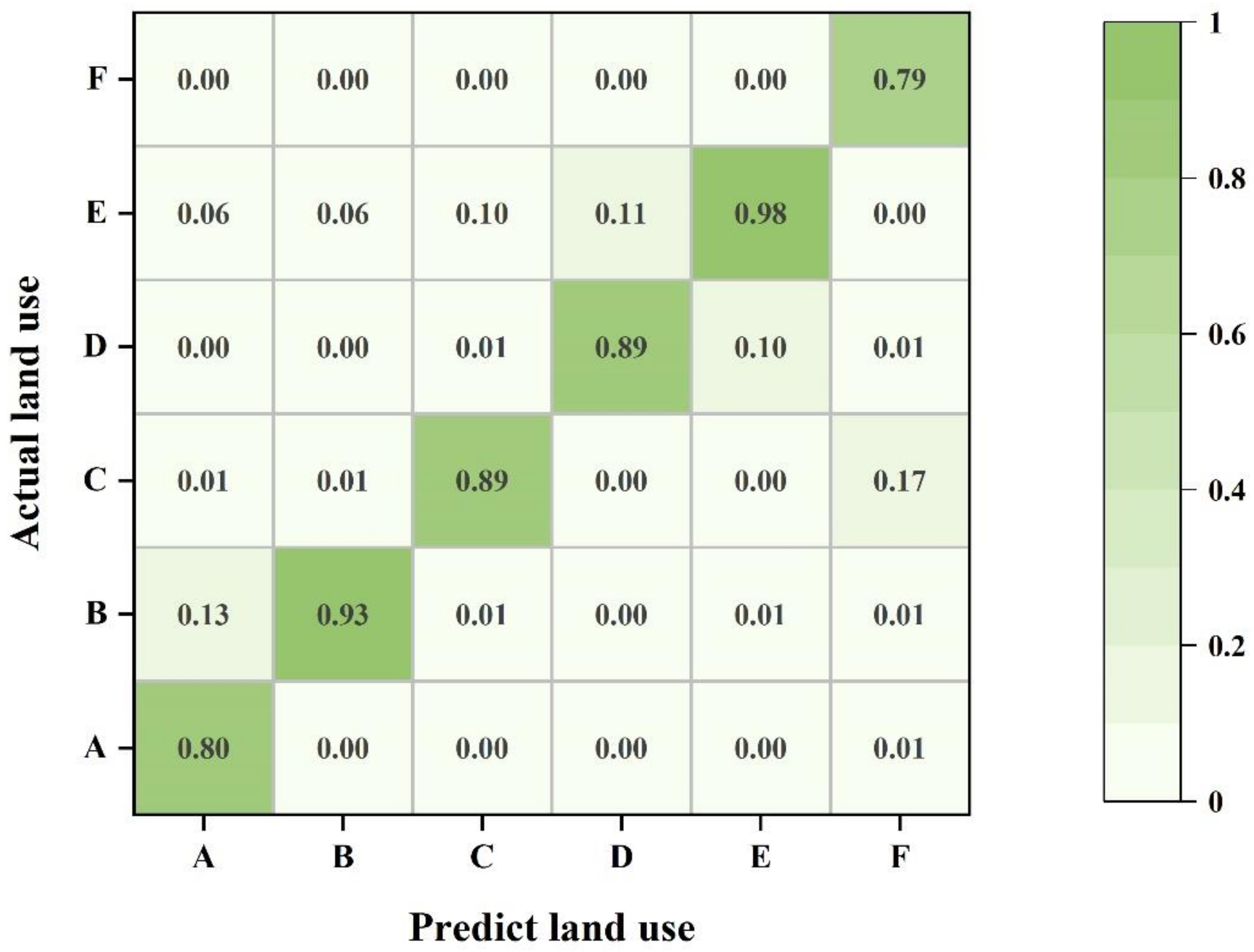
RSEI is employed to evaluate the regional ecological quality, which is a function of heat, greenness, humidity and dryness. The four parameters can be qualified by LST, NDVI, WET and NDBSI, respectively, which is expressed as Equation (4) [26,27]:

$$\mathrm{RSEI}=\mathrm{f}\left(\mathrm{Greenness},\mathrm{Wetness},\mathrm{Heat},\mathrm{Dryness}\right)=\mathrm{f}\left(\mathrm{NDVI},\mathrm{WET},\mathrm{LST},\mathrm{NDBSI}\right)$$

(4)

NDBSI and WET are calculated from MOD09GA daily surface reflectance data. NDBSI is the mean value of IBI (index-based built-up index) and SI (soil index), which is calculated as in Equations (5)–(7) [26,27,70,71]; WET index is obtained as in Equation (8) [71,72]:

$$\mathrm{NDBSI}=\frac{\mathrm{IBI}+\mathrm{SI}}{2}$$

(5)

$$\mathrm{IBI}=\frac{\frac{{2\mathsf{\rho }}_{\mathrm{SWIR}}}{{\mathsf{\rho }}_{\mathrm{SWIR}}{+\mathsf{\rho }}_{\mathrm{NIR}}}-\left(\frac{{\mathsf{\rho }}_{\mathrm{NIR}}}{{\mathsf{\rho }}_{\mathrm{Red}}{+\mathsf{\rho }}_{\mathrm{NIR}}}+\frac{{\mathsf{\rho }}_{\mathrm{Green}}}{{\mathsf{\rho }}_{\mathrm{Green}}{+\mathsf{\rho }}_{\mathrm{SWIR}}}\right)}{\frac{{2\mathsf{\rho }}_{\mathrm{SWIR}}}{{\mathsf{\rho }}_{\mathrm{SWIR}}{+\mathsf{\rho }}_{\mathrm{NIR}}}+\left(\frac{{\mathsf{\rho }}_{\mathrm{NIR}}}{{\mathsf{\rho }}_{\mathrm{Red}}{+\mathsf{\rho }}_{\mathrm{NIR}}}+\frac{{\mathsf{\rho }}_{\mathrm{Green}}}{{\mathsf{\rho }}_{\mathrm{Green}}{+\mathsf{\rho }}_{\mathrm{SWIR}}}\right)}$$

(6)

$$\mathrm{SI}=\frac{\left({\mathsf{\rho }}_{\mathrm{SWIR}}{+\mathsf{\rho }}_{\mathrm{Red}}\right)-\left({\mathsf{\rho }}_{\mathrm{NIR}}{+\mathsf{\rho }}_{\mathrm{Blue}}\right)}{\left({\mathsf{\rho }}_{\mathrm{SWIR}}{+\mathsf{\rho }}_{\mathrm{Red}}\right)+\left({\mathsf{\rho }}_{\mathrm{NIR}}{+\mathsf{\rho }}_{\mathrm{Blue}}\right)}$$

(7)

$$\mathrm{Wet}=0{.1147\mathsf{\rho }}_{\mathrm{Red}}+0{.2489\mathsf{\rho }}_{\mathrm{NIR}}+0{.2408\mathsf{\rho }}_{\mathrm{Blue}}+0{.3132\mathsf{\rho }}_{\mathrm{Green}}-0{.3122\mathsf{\rho }}_{\mathrm{NIR}2}-0{.6416\mathsf{\rho }}_{\mathrm{SWIR}}-0{.5087\mathsf{\rho }}_{\mathrm{SWIR}2}$$

(8)

where, ρ_Red, ρ_NIR, ρ_Blue, ρ_Green, ρ_NIR2, ρ_SWIR and ρ_SWIR2 are the reflectance of red band, NIR1 (near-infrared band1), blue band, green band, NIR2, SWIR1 (short-wave infrared band1) and SWIR2, respectively.

For the four factors, NDVI, WET, NDBSI and LST, the data were normalized by the normalization Equation (9) to the interval of [0, 1]. Then, principal component analysis (PCA) was performed on the four factors to obtain RSEI:

$${\mathrm{AX}}_{\mathrm{i}}=\frac{{\mathrm{X}}_{\mathrm{i}}{-\mathrm{X}}_{\min }}{{\mathrm{X}}_{\max }{-\mathrm{X}}_{\min }}$$

(9)

where, AX_i, X_i, X_min and X_max are the normalized values of an indicator, the value at image i and the minimum and the maximum value of the indicator, respectively.

The result of PCA shows that the average proportion of PC1 occupied feature values is greater than 83% (

Table 2. Eigen components and eigen proportions of PC1.

Index	2000 PC1	2003 PC1	2006 PC1	2009 PC1	2012 PC1	2015 PC1	2017 PC1	2020 PC1
NDVI	−0.343	−0.327	−0.356	−0.381	−0.321	−0.284	−0.329	−0.337
Wet	−0.380	−0.379	−0.378	−0.333	−0.386	−0.413	−0.390	−0.419
LST	0.620	0.635	0.652	0.694	0.614	0.582	0.629	0.557
NDBSI	0.594	0.635	0.553	0.513	0.609	0.640	0.587	0.633
Eigen proportions (%)	84.42	83.89	79.46	78.21	85.34	86.36	85.15	83.63

), and then PC1 is used as RSEI₀. The smaller value of RSEI₀ indicates better ecology quality. To make a large value indicate good ecology, the obtained RSEI₀ is subtracted from 1 to obtain RSEI₁, as in Equation (10):

$${\mathrm{RSEI}}_1{=1-\mathrm{RSEI}}_0=1-\mathrm{PC}1\left[\mathrm{f}\left(\mathrm{NDVI},\mathrm{WET},\mathrm{LST},\mathrm{NDBSI}\right)\right]$$

(10)

RSEI forecasting is based on historical data and varies along a time series, so there is a collinearity problem and strong covariance. The elastic network method (machine learning method) solves the collinearity problem better and explains the existence of strong covariance [73], so the elastic network regression is chosen as the RSEI prediction method. Accurate penalty methods yield good prediction performance of elastic network regression by deviation–variance trade-off [74]. There are two parameters, alpha and l1_ratio, that need to be adjusted. The prediction accuracy is judged by R² (coefficient of determination: it measures the goodness of fit, which means the predictive effect, by the proportion of variance explained): the higher the R² value, the better the fitting effect and the higher the prediction accuracy.

The 5000 random points are used as the ensemble of training and prediction samples for prediction, and the training and validation samples are set to 80% and 20% of the total number of samples, respectively. Based on the five-year plan time interval, the first four years were set as the independent variable X, and the fifth year was set as the dependent variable Y to go backward in prediction year by year, as in Equation (11). Based on the training and validation samples, the parameters alpha and l1_ratio were adjusted several times, and based on the R² results, alpha = 0.001 and l1_ratio = 0.5 were finally determined, and the R² obtained was 0.99. Taking 2011–2015 as an example, with the basin-wide prediction based on the elastic network regression model already obtained, the RSEI of 2011–2014 as the independent variable, resulting in an R2 of 0.96 between the 2015 prediction and the actual RSEI data.

$${\mathrm{RSEI}}_{\mathrm{t}}=\mathrm{f}\left({\mathrm{RSEI}}_{\mathrm{t}-1}{,\mathrm{RSEI}}_{\mathrm{t}-2}{,\mathrm{RSEI}}_{\mathrm{t}-3}{,\mathrm{RSEI}}_{\mathrm{t}-4}\right)$$

(11)

2.7. Validation

ROC values greater than 0.7 are generally considered a good fit [65]. The ROC values of farmland, forest, grassland, water, build-up land and unutilized land in this study were all greater than 0.7, indicating that the explanatory power of the drivers for each land-use type was strong. Besides, the Kappa coefficient between the actual land-use data and the predicted land-use results in 2011 was 0.93, with an overall accuracy of 0.98, showing high accuracy of the predicted results (Figure 3).

The relationships between RSEI and the four indices of LST, NDBSI, NDVI and WET in the HRB were shown in Figure 4. The results indicated that the RSEI of the HRB was negatively correlated with LST and NDBSI indexes and positively related to NDVI and WET indexes. It is proved that these four indices are available for calculating the RSEI in the HRB.

The four indicators, LST, NDVI, WET and NDBSI, were predicted by using elastic network regression, and then the indirect forecast results of RSEI^pca₂₀₃₅ were obtained by PCA. R² of RSEI₂₀₃₅ obtained from the direct forecast and the indirect forecast result of RSEI^pca₂₀₃₅ was calculated as 0.97, which proved that the consistency between the direct and indirect forecast results of RSEI in 2035 was high, and the elastic network regression was applicable to the RSEI forecast.

3. Results

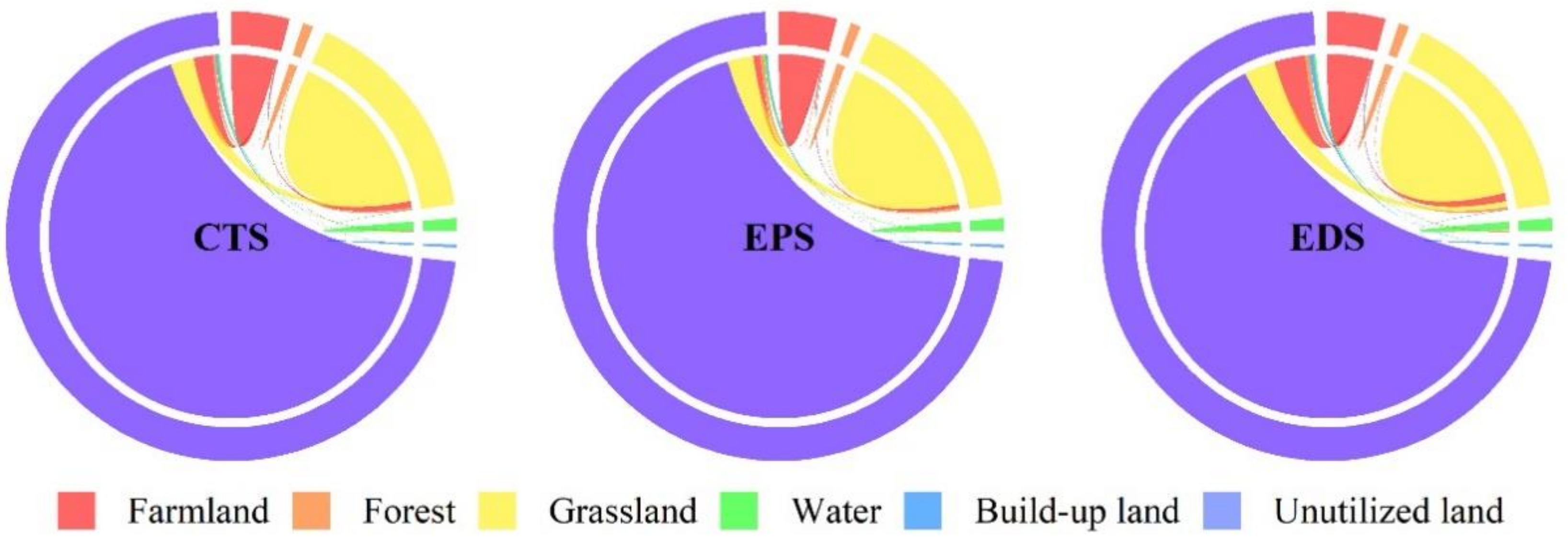
3.1. Projected Land-Use Changes

The results show that, compared with the year 2000 (Figure 5a), the total areas of farmland, forest, grassland, water and build-up land increase by 16.20%, 12.15% and 26.12% by 2035 for the three scenarios including CTS, EPS and EDS, respectively (Figure 5) (

Table 3. Area of each land-use type in 2000, 2011 and 2035 (ha).

	2000	2011	2035CTS	2035EPS	2035EDS
Farmland (ha)	619,300	709,400	905,981.82	689,248.76	1,088,336.36
Forest (ha)	127,700	146,500	187,518.18	207,450.37	220,245.45
Grassland (ha)	2,355,900	2,394,400	2,478,400	2,558,205.49	2,562,200
Water (ha)	156,000	160,200	169,363.64	169,363.64	169,363.64
Build-up land (ha)	36,200	52,400	87,745.45	70,072.73	115,654.55
Unutilized land (ha)	10,763,800	10,596,000	10,229,890.91	10,364,559.02	9,903,100
Total (ha)	14,058,900	14,058,900	14,058,900	14,058,900	14,058,900

). Comparing the actual land-use result (Figure 5b) with the predicted result (Figure 5c) in 2011, it can be seen that the simulation results are highly accurate.

Under CTS (Figure 5d), unutilized land and a small portion of grassland were converted to farmland, and farmland was the main land type to inflow. Compared with 2000, farmland increased by 286,681.82 ha in the whole basin, with a significant increase in the midstream area. The area of forest and grassland increased by 46.84% and 5.20%, respectively, and the forest area increased more in the upstream area. After the successful implementation of the Heihe River Basin ecological water diversion project in 2000, the downstream diversion of water increased the area of riparian forests and riparian wetlands, maintained a lake of 30 km² and a larger wetland ecosystem for the continuous injection of water into the Juyan lake and caused a slow increase in the overall body of water, with growth rates of 8.57% and 142.39% for water and construction land, respectively.

The increase of forest and grassland areas for the EPS (Figure 5e) is greater than the CTS, and the growth rate of green space area was 4.02% higher than the CTS. However, the growth rates of farmland and build-up land were 34.99% and 48.82% smaller than the CTS. The growth of water resources is the same as in the CTS.

Due to the economic dominance of the EDS (Figure 5f), the area of farmland and build-up land was much larger than the other two scenarios, with growth rates 29.45% and 77.10% higher than the CTS, mainly in the midstream region. The increase in forest and grassland areas is similar to EPS.

Figure 6 shows that with unutilized land as the main transfer out, the EDS transfers out the most, CTS the second and EPS the least. Under the CTS, the area of farmland and grassland increased the most, with smaller amounts of forest, water and build-up land, and a small amount of grassland was converted to farmland. The increase of farmland area under EDS is significantly more than that of forest, grassland, water and build-up land, the increase of build-up land is higher than the other two scenarios and the increase of the ratio of forest area is lower than that of the CTS. The percentage of green space conversion is the largest under the EPS, and the increase of farmland and build-up land is much lower than that of the CTS and EDS.

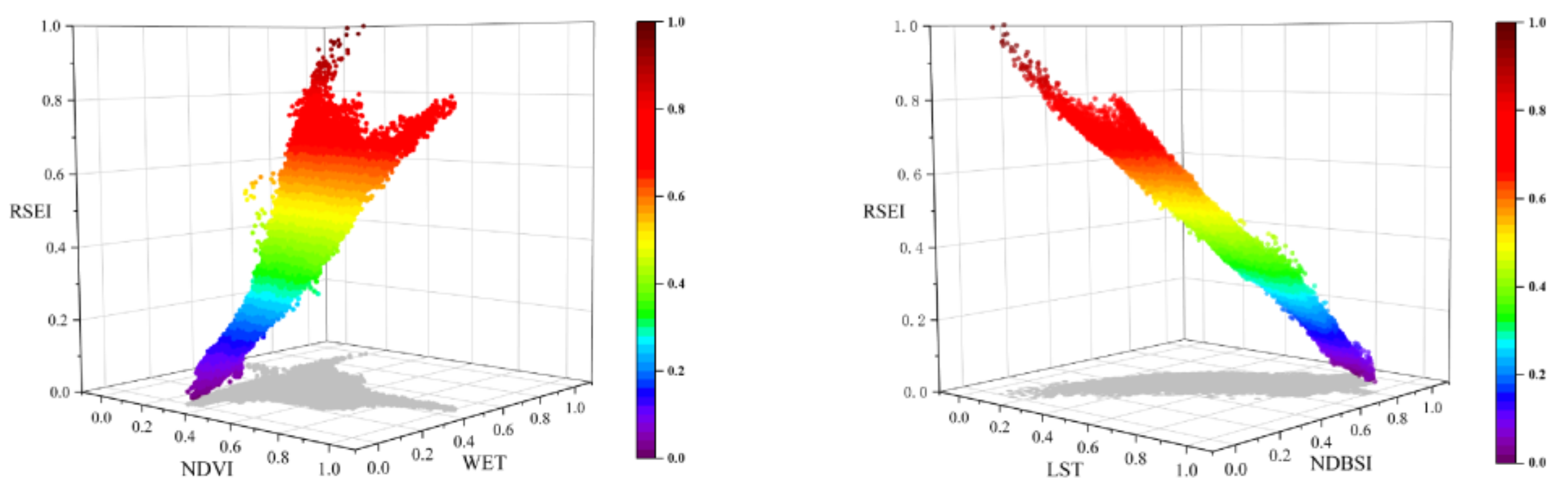
3.2. RSEI Prediction Results

The RSEI prediction results show that the ecological quality gradually turns better in 2035 (Figure 7). Compared with 2000 (Figure 7a), the RSEI values at the junction of the downstream and midstream areas in 2011 (Figure 7b) gradually become larger, indicating a gradual improvement in ecological quality and the reappearance of the Juyan lake in the downstream area after the diversion of the Heihe River. The RSEI data obtained from the indirect prediction (Figure 7d) differ little from the direct prediction data (Figure 7c), showing that the reliability of the elastic network regression for the prediction of RSEI data is high. In 2035, the quality of the ecological environment is better than that in 2000, and the mean value of the RSEI in the western part of the downstream area is improved from about 0.3 to 0.5, the ecological quality in the midstream area improves along the neighboring areas and the ecological environment in the downstream area near Juyan lake also improves.

3.3. Ecological Correspondence of Different Land-Use Scenarios

To understand the distribution of land-use changes and RSEI values under different scenarios of the HRB, each land-use type was analyzed and the RSEI values under different land-use scenarios were compared (Figure 8).

The distribution of RSEI values on farmland under the three scenarios showed that the RSEI values of farmland were distributed in the range of 0–0.7, where the area was mainly concentrated in the range of 0.3–0.4 with poor ecological quality. The comparison shows that, within the same RSEI value interval, the farmland area of the EDS is the largest, CTS is the second and EPS is the smallest.

The RSEI values are distributed over the forest land in the range of 0–0.8. In the range of 0–0.4, the forest area under the EPS is much larger than the other two scenarios, indicating that the EPS is most beneficial to the expansion of the forest extent in the ecologically poorer areas. In the interval of 0.4–0.8, the forest area under the EDS is larger than the other two scenarios, which means that the forest area under the EDS is larger than the other two scenarios in ecologically better areas. The RSEI distribution range of forest area under the CTS is in between the EPS and EDS.

A relatively consistent distribution of grassland area under the three scenarios, with most of the area within the value range of 0.3–0.8, indicates that the vast majority of grasslands are distributed in the ecologically average and ecologically better areas. The area under the EPS is larger in the ecologically poorer part, and the area under the EDS is larger in the ecologically better interval.

The RSEI distribution range of the area of water is wide, with distribution within 0–1, and most of them are located between 0.3 and 0.8, indicating that the ecological quality of the area where the water is located is good, and the distribution trends are similar in the three scenarios.

As for the area of build-up land, the RSEI values are mainly in the interval of 0–0.6, with little distribution in the interval of 0.6–0.8. Among the three scenarios, the percentage of build-up land under the EPS is the smallest, CTS is in the middle and the area under the EDS is the largest.

Unutilized land has the largest proportion of the HRB, and the majority of the RSEI values are distributed in the ecologically undesirable interval (RSEI values are located in the 0–0.2), which is consistent with the actual land use. The rate of change is lower than that of other land-use types, since the area of unutilized land occupies the largest proportion of the entire basin. The area of unutilized land changed the most under the EDS, followed by CTS and the least under EPS.

4. Discussion

The results of the RSEI synergistic multi-scenario analysis show that from 2000 to 2035, the main transferred land types are unutilized land, and there are various increases in farmland, forest, grassland, water and build-up land. The increase of forest, grassland and water area improves the ecological quality of the HRB, and the unutilized land and build-up land hurt the ecological environment. To more fully determine ecological quality, subsequent studies could include parameters such as biodiversity and adjust land management approaches to maintain regional ecological sustainability by understanding the composition of vegetation near watershed land types [75].

4.1. Spatial Impact of Land-Use Changes on Ecological Quality

According to the relationship between land-use changes and the driving factors, it can be seen that GDP, precipitation and temperature are the main driving factors of land-use change. Green space drives better ecological quality and is widely distributed in the upstream area where slope and temperature are low, so there is an increasing trend in the upstream, southern midstream and downstream areas along the water system of green space, which will promote the continuous optimization of ecological quality in green space areas. The upstream area is the origin of the Heihe River and has more precipitation than the midstream and downstream areas. Water has a positive impact on the ecological quality, and the ecological quality of the upstream area is the best, the midstream area is the second and the downstream area is the worst. Farmland is mainly distributed in the midstream area along the plain of the Hexi Corridor where the slope is small, the precipitation is medium and the GDP is relatively high. Since economy is the key factor influencing anthropogenic changes in land-use types [76,77], build-up land is mainly distributed in the midstream area of the HRB, driven by GDP. Under the combined effect of farmland and build-up land, the ecological condition in the midstream area is worse than that in the upstream area, and the ecological environment quality is medium. Low precipitation and high evaporation lead to a poor and uninhabitable ecological environment in the downstream area. Driven by both nature and societal factors, the economic development of the downstream area is slow, making the downstream area mostly unutilized land.

4.2. Ecological Quality of the Response to Multi-scenario Land-Use Changes

Under the CTS, EPS, and EDS, the area of the five land-use types that shifted from unutilized land accounted for 3.80%, 2.84% and 6.12% of the total basin area, respectively. The turn-in rate of each type is at a medium level under the CTS compared to the other two scenarios, with farmland and grassland being the main types of transfer. Under the EPS, 70.65% of the total transferred area is green space, which is beneficial for ecologically sustainable development. In the EDS, the increase of farmland and build-up land is significantly higher than the other two scenarios. When the mean value of the RSEI in the HRB is only 0.2, farmland can slightly improve the regional ecological quality, but when the value is in the middle range, farmland will no longer have a positive impact on the regional ecological quality, and the area of farmland should be limited to a reasonable range.

4.3. Policies Responding to Prediction Results

The ecological quality of build-up land and farmland distribution areas is poor; thus, the issues of limiting the expansion and efficiency of build-up land and farmland deserve to be taken seriously. The improvement of build-up land efficiency and rational arrangement of layout in urban planning [78] can effectively reduce the expansion of build-up land, thus reducing the harm of build-up land to the ecological environment. The predicted RSEI data can be used to guide policies in local areas, using various policies according to land-use changes, maintaining existing ecological protection policies in the upstream area of the HRB and implementing policies such as agricultural water coordination and reforestation in the midstream area and making corresponding policies in the downstream area for ecological protection around a rump lake and water use allocation in the whole basin.

4.4. Advantage and Disadvantage of the Integration Framework

In this study, the Dyna-CLUE model was used to predict the 2035 land-use data of the HRB, but the sudden appearance of a local land-use type, such as the recurrence of a rump lake in the downstream area of the HRB, was not easily predicted by it. The inability to verify the forecast results is a persistent problem in the forecasting work. Therefore, in our research, the goodness-of-fit of two RSEI results for 2035 are obtained by direct prediction, and the indirect prediction is 0.97. Then, the accuracy of the prediction results can corroborate each other. The prediction framework provides a quantitative analysis of the effects of land-use changes on ecological quality in (semi) arid regions and provide a useful reference for the follow-up work of this paper and similar studies in the future, whether the ideas and methods in the article apply to other regions and other climate type needs to be further explored.

5. Conclusions

Land-use changes driven by multiple factors and ecological quality responses to land-use changes are important foundations for future land-use management and ecological improvement. Unutilized land, farmland expansion and increasing urbanization are responsible for the lack of significant improvement in the overall ecological quality in the HRB. Therefore, we propose a prediction framework based on land-use changes and ecological quality. Under this framework, the effects of each land-use type on ecological quality under three scenarios were analyzed and compared based on the Dyna-CLUE model and the elastic network regression method. The following conclusions were drawn: (I) Driven by the factors such as GDP, precipitation and temperature, the total area of unutilized land turned out to be 3.80%, 2.84% and 6.12% of the total basin under the CTS, EPS and EDS, respectively, compared to the year 2000. Those indicate that the main trend of future land-use changes is the transfer out of unutilized land and the corresponding increase in farmland, forest, grassland, water and build-up land. (II) The positive effects of green spaces (grassland, forest) and water on ecological quality and negative effects of build-up land and unutilized land on ecological quality are significant. The improvement of ecological quality in areas with poor overall ecological conditions (RSEI ≤ 0.4) such as the HRB was obvious for agricultural land but not for areas with RSEI values greater than 0.4 (Figure 8), indicating that ecological quality changed as a result of land-use changes. (III) The framework is applicable to the Heihe River Basin, and the projections show that the policy orientation is to increase the green space coverage and improve the efficiency of land use for construction, farmland and water resources.

On the whole, this study spatially predicts and evaluates the trends of ecological quality changes under the influence from three land-use-change scenarios in a long-time series through the prediction framework, and this approach provides a basis for future land management and regional sustainable development policies. By coordinating different scenarios in the upstream, midstream and downstream areas and making water resource allocations, land-use distribution and ecological protection policies by region will help improve the ecological quality and comprehensive sustainable development of the whole basin.

References

1. Borrelli, P.; Robinson, D.A.; Panagos, P.; Lugato, E.; Yang, J.E.; Alewell, C.; Wuepper, D.; Montanarella, L.; Ballabio, C. Land use and climate change impacts on global soil erosion by water (2015–2070). Proc. Natl. Acad. Sci. USA 2020, 117, 21994–22001. [Google Scholar] [CrossRef]
2. Robinson, D.A.; Panagos, P.; Borrelli, P.; Jones, A.; Montanarella, L.; Tye, A.; Obst, C.G. Soil natural capital in europe; a framework for state and change assessment. Sci. Rep. 2017, 7, 6706. [Google Scholar] [CrossRef] [Green Version]
3. Shen, Q.; Gao, G.; Han, F.; Xiao, F.; Ma, Y.; Wang, S.; Fu, B. Quantifying the effects of human activities and climate variability on vegetation cover change in a hyper-arid endorheic basin. Land Degrad. Dev. 2018, 29, 3294–3304. [Google Scholar] [CrossRef]
4. Winkler, K.; Fuchs, R.; Rounsevell, M.; Herold, M. Global land use changes are four times greater than previously estimated. Nat. Commun. 2021, 12, 2501. [Google Scholar] [CrossRef] [PubMed]
5. Morton, D.C.; DeFries, R.S.; Shimabukuro, Y.E.; Anderson, L.O.; Arai, E.; del Bon Espirito-Santo, F.; Freitas, R.; Morisette, J. Cropland expansion changes deforestation dynamics in the southern brazilian amazon. Proc. Natl. Acad. Sci. USA 2006, 103, 14637–14641. [Google Scholar] [CrossRef] [PubMed] [Green Version]
6. Macedo, M.N.; DeFries, R.S.; Morton, D.C.; Stickler, C.M.; Galford, G.L.; Shimabukuro, Y.E. Decoupling of deforestation and soy production in the southern amazon during the late 2000s. Proc. Natl. Acad. Sci. USA 2012, 109, 1341–1346. [Google Scholar] [CrossRef] [Green Version]
7. Perz, S.G.; Qiu, Y.; Xia, Y.; Southworth, J.; Sun, J.; Marsik, M.; Rocha, K.; Passos, V.; Rojas, D.; Alarcón, G.; et al. Trans-boundary infrastructure and land cover change: Highway paving and community-level deforestation in a tri-national frontier in the amazon. Land Use Policy 2013, 34, 27–41. [Google Scholar] [CrossRef]
8. Montoya, A.; de Lima, A.; Adami, M. Analysis of the land cover around a hydroelectric power plant in the brazilian amazon. Anu. Inst. Geociênc 2019, 42, 74–86. [Google Scholar] [CrossRef]
9. Xu, X.; Xie, Y.; Qi, K.; Luo, Z.; Wang, X. Detecting the response of bird communities and biodiversity to habitat loss and fragmentation due to urbanization. Sci. Total Environ. 2018, 624, 1561–1576. [Google Scholar] [CrossRef]
10. Llerena-Montoya, S.; Velastegui-Montoya, A.; Zhirzhan-Azanza, B.; Herrera-Matamoros, V.; Adami, M.; de Lima, A.; Moscoso-Silva, F.; Encalada, L. Multitemporal analysis of land use and land cover within an oil block in the ecuadorian amazon. ISPRS Int. J. Geo-Inf. 2021, 10, 191. [Google Scholar] [CrossRef]
11. Kamusoko, C.; Aniya, M.; Adi, B.; Manjoro, M. Rural sustainability under threat in zimbabwe–simulation of future land use/cover changes in the bindura district based on the markov-cellular automata model. Appl. Geogr. 2009, 29, 435–447. [Google Scholar] [CrossRef]
12. Sang, L.; Zhang, C.; Yang, J.; Zhu, D.; Yun, W. Simulation of land use spatial pattern of towns and villages based on ca–markov model. Math. Comput. Model. 2011, 54, 938–943. [Google Scholar] [CrossRef]
13. Subedi, P.; Subedi, K.; Thapa, B. Application of a hybrid cellular automaton–markov (ca-markov) model in land-use change prediction: A case study of saddle creek drainage basin, florida. Appl. Ecol. Environ. Sci. 2013, 1, 126–132. [Google Scholar] [CrossRef] [Green Version]
14. Behera, M.D.; Borate, S.N.; Panda, S.N.; Behera, P.R.; Roy, P.S. Modelling and analyzing the watershed dynamics using cellular automata (ca)–markov model–a geo-information based approach. J. Earth Syst. Sci. 2012, 121, 1011–1024. [Google Scholar] [CrossRef] [Green Version]
15. Nouri, J.; Gharagozlou, A.; Arjmandi, R.; Faryadi, S.; Adl, M. Predicting urban land use changes using a ca–markov model. Arab. J. Sci. Eng. 2014, 39, 5565–5573. [Google Scholar] [CrossRef]
16. Mansour, S.; Al-Belushi, M.; Al-Awadhi, T. Monitoring land use and land cover changes in the mountainous cities of oman using gis and ca-markov modelling techniques. Land Use Policy 2020, 91, 104414. [Google Scholar] [CrossRef]
17. Verburg, P.H.; Soepboer, W.; Veldkamp, A.; Limpiada, R.; Espaldon, V.; Mastura, S.S. Modeling the spatial dynamics of regional land use: The clue-s model. Environ. Manag. 2002, 30, 391–405. [Google Scholar] [CrossRef]
18. Verburg, P.H.; Veldkamp, A. Projecting land use transitions at forest fringes in the philippines at two spatial scales. Landsc. Ecol. 2004, 19, 77–98. [Google Scholar] [CrossRef]
19. Verburg, P.H.; Overmars, K.P. Combining top-down and bottom-up dynamics in land use modeling: Exploring the future of abandoned farmlands in europe with the dyna-clue model. Landsc. Ecol. 2009, 24, 1167–1181. [Google Scholar] [CrossRef]
20. Lima, M.L.; Zelaya, K.; Massone, H. Groundwater vulnerability assessment combining the drastic and dyna-clue model in the argentine pampas. Environ. Manag. 2011, 47, 828–839. [Google Scholar] [CrossRef]
21. Sakayarote, K.; Shrestha, R.P. Simulating land use for protecting food crop areas in northeast thailand using gis and dyna-clue. J. Geogr. Sci. 2019, 29, 803–817. [Google Scholar] [CrossRef] [Green Version]
22. Waiyasusri, K.; Wetchayont, P. Assessing long-term deforestation in nam san watershed, loei province, thailand using a dyna-clue model. Geogr. Environ. Sustain. 2020, 13, 81–97. [Google Scholar] [CrossRef]
23. Wang, Y.; Chao, B.; Dong, P.; Zhang, D.; Yu, W.; Hu, W.; Ma, Z.; Chen, G.; Liu, Z.; Chen, B. Simulating spatial change of mangrove habitat under the impact of coastal land use: Coupling maxent and dyna-clue models. Sci. Total Environ. 2021, 788, 147914. [Google Scholar] [CrossRef] [PubMed]
24. Liu, J.; Zhang, Z.; Xu, X.; Kuang, W.; Zhou, W.; Zhang, S.; Li, R.; Yan, C.; Yu, D.; Wu, S.; et al. Spatial patterns and driving forces of land use change in china during the early 21st century. J. Geogr. Sci. 2010, 20, 483–494. [Google Scholar] [CrossRef]
25. De Keersmaecker, W.; Lhermitte, S.; Honnay, O.; Farifteh, J.; Somers, B.; Coppin, P. How to measure ecosystem stability? An evaluation of the reliability of stability metrics based on remote sensing time series across the major global ecosystems. Glob. Change Biol. 2014, 20, 2149–2161. [Google Scholar] [CrossRef] [PubMed]
26. Xu, H. A remote sensing urban ecological index and its application. Acta Ecol. Sin. 2013, 33, 7853–7862. [Google Scholar] [CrossRef]
27. Xu, H. Remote sensing evaluation index of regional ecological environment change. China Environ. Sci. 2013, 33, 889–897. [Google Scholar]
28. Xu, H.; Wang, M.; Shi, T.; Guan, H.; Fang, C.; Lin, Z. Prediction of ecological effects of potential population and impervious surface increases using a remote sensing based ecological index (rsei). Ecol. Indic. 2018, 93, 730–740. [Google Scholar] [CrossRef]
29. Yuan, B.; Fu, L.; Zou, Y.; Zhang, S.; Chen, X.; Li, F.; Deng, Z.; Xie, Y. Spatiotemporal change detection of ecological quality and the associated affecting factors in dongting lake basin, based on rsei. J. Clean. Prod. 2021, 302, 126995. [Google Scholar] [CrossRef]
30. Xiong, Y.; Xu, W.; Lu, N.; Huang, S.; Wu, C.; Wang, L.; Dai, F.; Kou, W. Assessment of spatial–temporal changes of ecological environment quality based on rsei and gee: A case study in erhai lake basin, yunnan province, china. Ecol. Indic. 2021, 125, 107518. [Google Scholar] [CrossRef]
31. Zhu, D.; Chen, T.; Zhen, N.; Niu, R. Monitoring the effects of open-pit mining on the eco-environment using a moving window-based remote sensing ecological index. Environ. Sci. Pollut. Res. 2020, 27, 15716–15728. [Google Scholar] [CrossRef] [PubMed]
32. Hu, X.; Xu, H. A new remote sensing index for assessing the spatial heterogeneity in urban ecological quality: A case from fuzhou city, china. Ecol. Indic. 2018, 89, 11–21. [Google Scholar] [CrossRef]
33. Gou, R.; Zhao, J. Eco-environmental quality monitoring in beijing, china, using an rsei-based approach combined with random forest algorithms. IEEE Access 2020, 8, 196657–196666. [Google Scholar] [CrossRef]
34. Ariken, M.; Zhang, F.; Liu, K.; Fang, C.; Kung, H.-T. Coupling coordination analysis of urbanization and eco-environment in yanqi basin based on multi-source remote sensing data. Ecol. Indic. 2020, 114, 106331. [Google Scholar] [CrossRef]
35. Yang, H.; Zhong, X.; Deng, S.; Xu, H. Assessment of the impact of lucc on npp and its influencing factors in the yangtze river basin, china. CATENA 2021, 206, 105542. [Google Scholar] [CrossRef]
36. Hou, K.; Wen, J. Quantitative analysis of the relationship between land use and urbanization development in typical arid areas. Environ. Sci. Pollut. Res. 2020, 27, 38758–38768. [Google Scholar] [CrossRef]
37. Wang, J.; Liu, Y.; Li, Y. Ecological restoration under rural restructuring: A case study of yan’an in china’s loess plateau. Land Use Policy 2019, 87, 104087. [Google Scholar] [CrossRef]
38. Xiao, S.; Xiao, H. The impact of human activity on the water environment of heihe water basin in last century. J. Arid Land Resour. Environ. 2004, 18, 57–62. [Google Scholar] [CrossRef]
39. Zhang, M.; Wang, S.; Fu, B.; Gao, G.; Shen, Q. Ecological effects and potential risks of the water diversion project in the heihe river basin. Sci. Total Environ. 2018, 619-620, 794–803. [Google Scholar] [CrossRef]
40. Wang, F.; Pan, X.; Wang, D.; Shen, C.; Lu, Q. Combating desertification in china: Past, present and future. Land Use Policy 2013, 31, 311–313. [Google Scholar] [CrossRef]
41. Wang, X.M.; Zhang, C.X.; Hasi, E.; Dong, Z.B. Has the three norths forest shelterbelt program solved the desertification and dust storm problems in arid and semiarid china? J. Arid Environ. 2010, 74, 13–22. [Google Scholar] [CrossRef]
42. Yin, H.; Pflugmacher, D.; Li, A.; Li, Z.; Hostert, P. Land use and land cover change in inner mongolia—Understanding the effects of china’s re-vegetation programs. Remote Sens. Environ. 2018, 204, 918–930. [Google Scholar] [CrossRef]
43. Li, X.; Cheng, G.; Liu, S.; Xiao, Q.; Ma, M.; Jin, R.; Che, T.; Liu, Q.; Wang, W.; Qi, Y. Heihe watershed allied telemetry experimental research (hiwater): Scientific objectives and experimental design. Bull. Am. Meteorol. Soc. 2013, 94, 1145–1160. [Google Scholar] [CrossRef]
44. Ge, Y.; Li, X.; Tian, W.; Zhang, Y.; Wang, W.; Hu, X. The impacts of water delivery on artificial hydrological circulation system of the middle reaches of the heihe river basin. Adv. Earth Sci. 2014, 29, 285. [Google Scholar] [CrossRef]
45. Li, X.; Cheng, G.; Ge, Y.; Li, H.; Han, F.; Hu, X.; Tian, W.; Tian, Y.; Pan, X.; Nian, Y. Hydrological cycle in the heihe river basin and its implication for water resource management in endorheic basins. J. Geophys. Res. Atmos. 2018, 123, 890–914. [Google Scholar] [CrossRef]
46. Jianhua, W. Landuse/Landcover Data of the Heihe River Basin in 2000; National Tibetan Plateau Data Center: Beijing, China, 2015. [Google Scholar] [CrossRef]
47. Hu, X.; Lu, L.; Li, X.; Wang, J.; Guo, M. Land use/cover change in the middle reaches of the heihe river basin over 2000–2011 and its implications for sustainable water resource management. PLoS ONE 2015, 10, e0128960. [Google Scholar] [CrossRef]
48. Jianhua, W. Landuse/Landcover Data of the Heihe River Basin (2011); National Tibetan Plateau Data Center: Beijing, China, 2014. [Google Scholar] [CrossRef]
49. National Basic Geographic Information Center. 1km Dem Dataset in the Heihe River Basin (2011); National Tibetan Plateau Data Center: Beijing, China, 2013. [Google Scholar]
50. Na, Z.; Tianxiang, Y. Monthly Mean Temperature for the Period (1961–2010); National Tibetan Plateau Data Center: Beijing, China, 2016. [Google Scholar] [CrossRef]
51. Zhao, N.; Yue, T.; Zhou, X.; Zhao, M.; Liu, Y.; Du, Z.; Zhang, L. Statistical downscaling of precipitation using local regression and high accuracy surface modeling method. Theor. Appl. Climatol. 2017, 129, 281–292. [Google Scholar] [CrossRef]
52. Tianxiang, Y.; Na, Z. Monthly Mean Vegetation Index and Precipitation Data Set of Heihe River Basin (1961–2010); National Tibetan Plateau Data Center: Beijing, China, 2018. [Google Scholar] [CrossRef]
53. National Basic Geographic Information Center. Iver Network Dataset of the Heihe River Basin (2009); National Tibetan Plateau Data Center: Beijing, China, 2013. [Google Scholar]
54. Li, X.; Nan, Z.; Cheng, G.; Ding, Y.; Wu, L.; Wang, L.; Wang, J.; Ran, Y.; Li, H.; Pan, X. Toward an improved data stewardship and service for environmental and ecological science data in west china. Int. J. Digit. Earth 2011, 4, 347–359. [Google Scholar] [CrossRef]
55. Jun, Z. Dataset of the Heihe Social Economy (2000–2009); National Tibetan Plateau Data Center: Beijing, China, 2013. [Google Scholar]
56. Lizong, W.; Yanyun, N. Primary Road Network Dataset of the Heihe River Basin (2010); National Tibetan Plateau Data Center: Beijing, China, 2013. [Google Scholar]
57. National Basic Geographic Information Center. The Resident Site Distribution Data of the Heihe River Basin; National Tibetan Plateau Data Center: Beijing, China, 2013. [Google Scholar]
58. Xuemei, W.; Mingguo, M. Gridded Population Data of the Heihe River Basin (2000); National Tibetan Plateau Data Center: Beijing, China, 2013. [Google Scholar] [CrossRef]
59. Wang, X.; Ma, M. A distance variable to simulate the urban population. In Remote Sensing for Environmental Monitoring, GIS Applications, and Geology VII; International Society for Optics and Photonics: Bellingham, WA, USA, 2007; p. 67491S. [Google Scholar] [CrossRef]
60. Krisnayanti, D.S.; Bunganaen, W.; Frans, J.; Seran, Y.A.; Legono, D. Curve number estimation for ungauged watershed in semi-arid region. Civ. Eng. J. 2021, 7, 1070–1083. [Google Scholar] [CrossRef]
61. Feistel, R.; Hellmuth, O. Relative humidity: A control valve of the steam engine climate. J. Hum. Earth Future 2021, 2, 140–182. [Google Scholar] [CrossRef]
62. Ekwueme, B.N.; Agunwamba, J.C. Trend analysis and variability of air temperature and rainfall in regional river basins. Civ. Eng. J. 2021, 7. [Google Scholar] [CrossRef]
63. Chuanglin, F.; Chao, B. The coupling model of water-ecology-economy coordinated development and its application in heihe river basin. Acta Geogr. Sin. 2004, 59, 781–790. [Google Scholar] [CrossRef]
64. Ling, Z. Multiple-Scenario Analyses of Land Use Change and Hydrological Responses in the Heihe River Basin. Master’s Thesis, University of Chinese Academy of Sciences, Beijing, China, 2014. [Google Scholar]
65. Lin, Y.-P.; Chu, H.-J.; Wu, C.-F.; Verburg, P.H. Predictive ability of logistic regression, auto-logistic regression and neural network models in empirical land-use change modeling—A case study. Int. J. Geogr. Inf. Sci. 2011, 25, 65–87. [Google Scholar] [CrossRef] [Green Version]
66. Pontius, R.G.; Schneider, L.C. Land-cover change model validation by an roc method for the ipswich watershed, massachusetts, USA. Agric. Ecosyst. Environ. 2001, 85, 239–248. [Google Scholar] [CrossRef]
67. Pontius, R.G. Quantification error versus location error in comparison of categorical maps. Photogramm. Eng. Remote Sens. 2000, 66, 1011–1016. [Google Scholar]
68. Congalton, R.G. A review of assessing the accuracy of classifications of remotely sensed data. Remote Sens. Environ. 1991, 37, 35–46. [Google Scholar] [CrossRef]
69. Foody, G.M. Status of land cover classification accuracy assessment. Remote Sens. Environ. 2002, 80, 185–201. [Google Scholar] [CrossRef]
70. Liao, W.; Jiang, W. Evaluation of the spatiotemporal variations in the eco-environmental quality in china based on the remote sensing ecological index. Remote Sens. 2020, 12, 2462. [Google Scholar] [CrossRef]
71. Xu, H.; Wang, Y.; Guan, H.; Shi, T.; Hu, X. Detecting ecological changes with a remote sensing based ecological index (rsei) produced time series and change vector analysis. Remote Sens. 2019, 11, 2345. [Google Scholar] [CrossRef] [Green Version]
72. Lobser, S.; Cohen, W. Modis tasselled cap: Land cover characteristics expressed through transformed modis data. Int. J. Remote Sens. 2007, 28, 5079–5101. [Google Scholar] [CrossRef]
73. Park, I.W.; Mazer, S.J. Overlooked climate parameters best predict flowering onset: Assessing phenological models using the elastic net. Glob. Change Biol. 2018, 24, 5972–5984. [Google Scholar] [CrossRef] [PubMed]
74. Zou, H.; Hastie, T. Regularization and variable selection via the elastic net. J. R. Stat. Soc. Ser. B 2005, 67, 301–320. [Google Scholar] [CrossRef] [Green Version]
75. Raposo, M.; Quinto-Canas, R.; Cano-Ortiz, A.; Spampinato, G.; Pinto Gomes, C. Originalities of willow of salix atrocinerea brot. In mediterranean europe. Sustainability 2020, 12, 8019. [Google Scholar] [CrossRef]
76. Shirmohammadi, B.; Malekian, A.; Salajegheh, A.; Taheri, B.; Azarnivand, H.; Malek, Z.; Verburg, P.H. Scenario analysis for integrated water resources management under future land use change in the urmia lake region, iran. Land Use Policy 2020, 90, 104299. [Google Scholar] [CrossRef]
77. Wang, X.; Zheng, D.; Shen, Y. Land use change and its driving forces on the tibetan plateau during 1990–2000. CATENA 2008, 72, 56–66. [Google Scholar] [CrossRef]
78. Song, H.M.; Xue, L. Dynamic monitoring and analysis of ecological environment in weinan city, northwest china based on rsei model. Ying Yong Sheng Tai Xue Bao 2016, 27, 3913–3919. [Google Scholar] [CrossRef]
Figure 1. Overview map of the study area (HRB).
Sustainability 14 02716 g001
Figure 2. Flow chart of each part and general framework.
Sustainability 14 02716 g002
Figure 3. Confusion matrix for land use prediction accuracy (A–F indicate farmland, forest, grassland, water, build-up land and unutilized land, respectively).
Sustainability 14 02716 g003
Figure 4. The 3D scatterplots of feature space.
Sustainability 14 02716 g004
Figure 5. Map of actual land-use data and predicted land-use data: (a) actual land-use data for 2000; (b) actual land-use data for 2011; (c) predicted land-use data for 2011; (d) predicted land-use data of CTS for 2035; (e) predicted land-use data of EPS for 2035; (f) predicted land-use data of EDS for 2035.
Sustainability 14 02716 g005
Figure 6. Land-use transfer relationships under CTS, EDS and EPS in HRB.
Sustainability 14 02716 g006
Figure 7. Map of actual RSEI and predicted RSEI (a). actual RSEI data for 2000; (b). actual RSEI data for 2011; (c). directly predicted RSEI data for 2035; (d). indirectly predicted RSEI data for 2035).
Sustainability 14 02716 g007
Figure 8. Distribution of RSEI values for farmland, forest, grassland, water, build-up land and unutilized land under three scenarios.
Sustainability 14 02716 g008