
Optimal Control of Energy Systems in Net-Zero Energy Buildings Considering Dynamic Costs: A Case Study of Zero Carbon Building in Hong Kong

 ,
,
Abstract
:1. Introduction
2. Methodology
3. Modeling of DCI-OM
3.1. Renewable Generations Models
3.2. Electric Vehicle Charging Station Model
3.3. Dynamic Cost Model
3.4. Integrated Demand Response Model
3.4.1. Demand Response of Electricity Load
3.4.2. Demand Response of Cooling Load
3.4.3. Evaluation Indexes for Demand Response
3.5. DCI-OM Mathematical Model
3.5.1. Objective Function
3.5.2. Constraints Conditions
- (1)
- Power supply system constraints
- (2)
- Cooling system constraints
- (1)
- The constraints for cooling power balancewhere, is the cooling load demand in time t, is the cooling power of the nth refrigeration unit in time t, N is the total number of refrigeration units, is the cooling power of the storage unit in time t, is the cooling power of the storage unit in time t.
- (2)
- Constraints for the operation of the refrigeration unitwhere, is the power consumption of the nth refrigeration unit at time t, is the rated cooling power of the nth refrigeration unit; is the performance coefficient of the refrigeration unit.
- (3)
- Constraints for cold storage
3.6. Comparison of Optimization Options
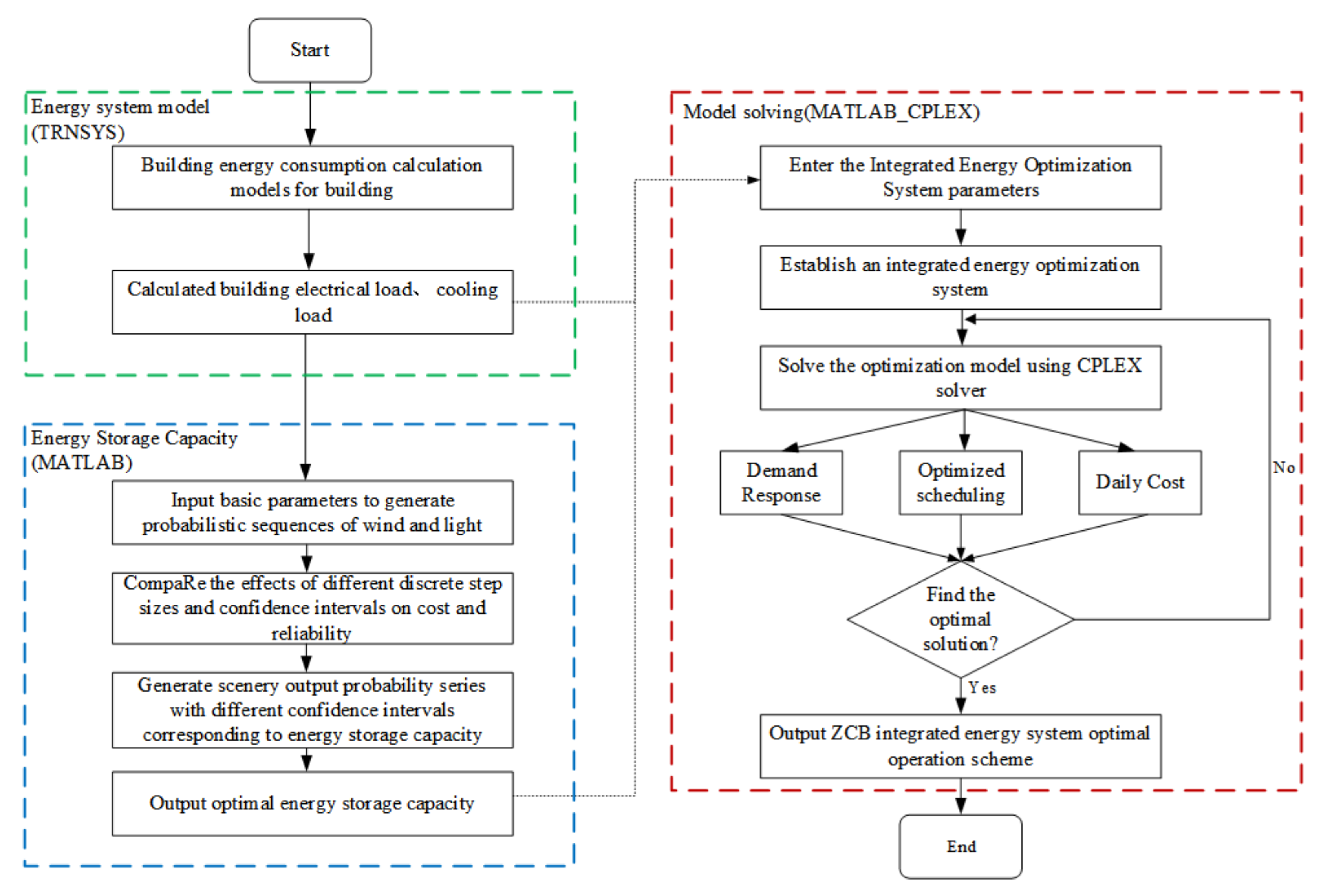
3.7. DCI-OM Model Solving
4. Case Study
4.1. Model Parameters Settings
- (1)
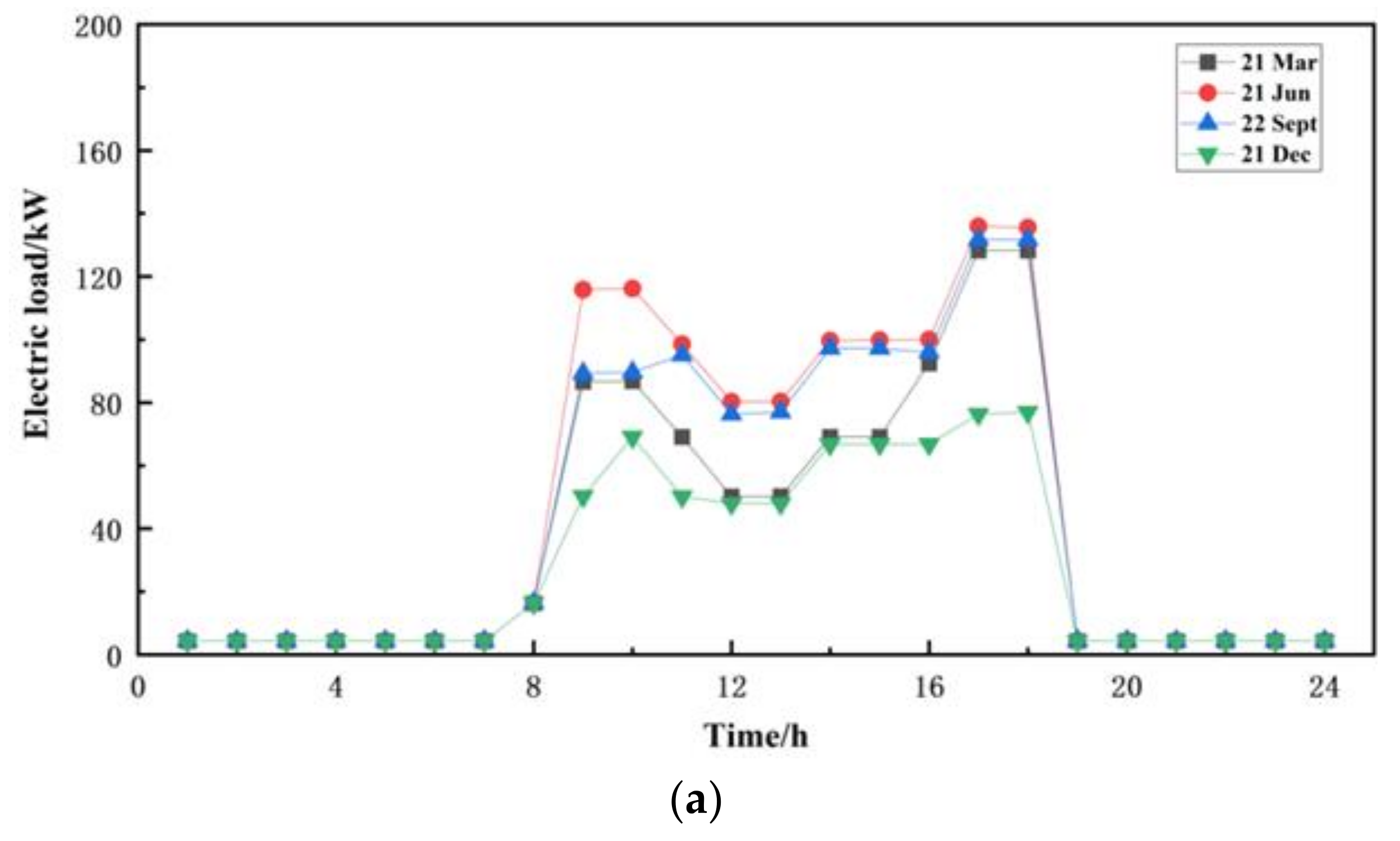
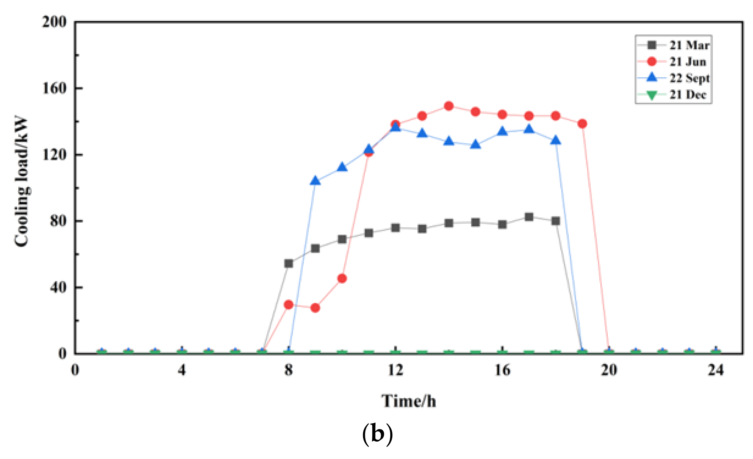
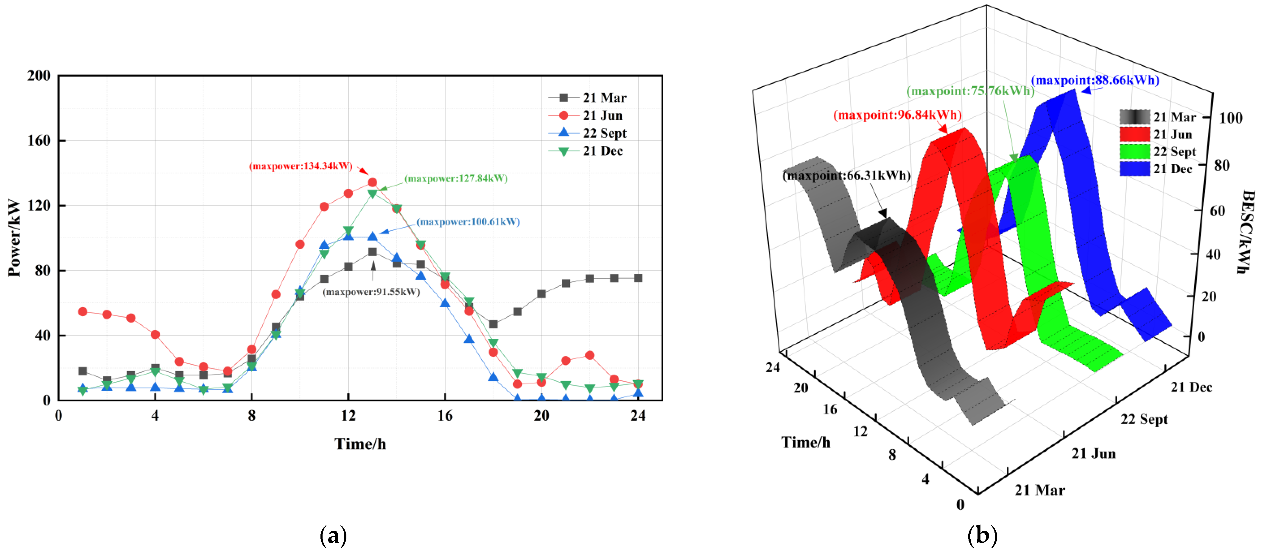
- Load parameters: four typical daily loads are calculated on TRNSYS. Since Hong Kong is located in a subtropical climate with high winter temperatures and long cooling periods throughout the year, only the electricity and cooling loads are considered in this study. The calculated electricity and cooling loads are shown in Figure 5.
- (2)
- Grid parameters: the maximum power provided by the grid for the system is 100 kW.
- (3)
- Cold storage device parameters: , , the maximum and minimum storage(CSC)/discharge(CSS) power are both 75 kW.
- (4)
- Refrigeration unit parameters: the system contains two refrigeration units (i.e., absorption refrigeration chiller, ground source heat pump), the rated power of the refrigeration output is both 100 kW, the cooling performance coefficient (COP) of absorption refrigeration chiller (ABC) and ground source heat pump (ELC) are 3.5 and 5, respectively.
- (5)
- Electric vehicle charging station parameters: the system contains one charging station with 10 charging posts, each with a charging power of 15 kW. A total of 15 electric vehicles are assumed in the office area, each with a battery capacity of 60 kWh. Total charging power of 900 kW is assumed for electric vehicles in one dispatch cycle, and the probability model of disorderly charging of electric vehicles in this study refers to the literature [32], i.e., . The joint probability density of arrival and departure of EVs is shown in Figure 6.
- (6)
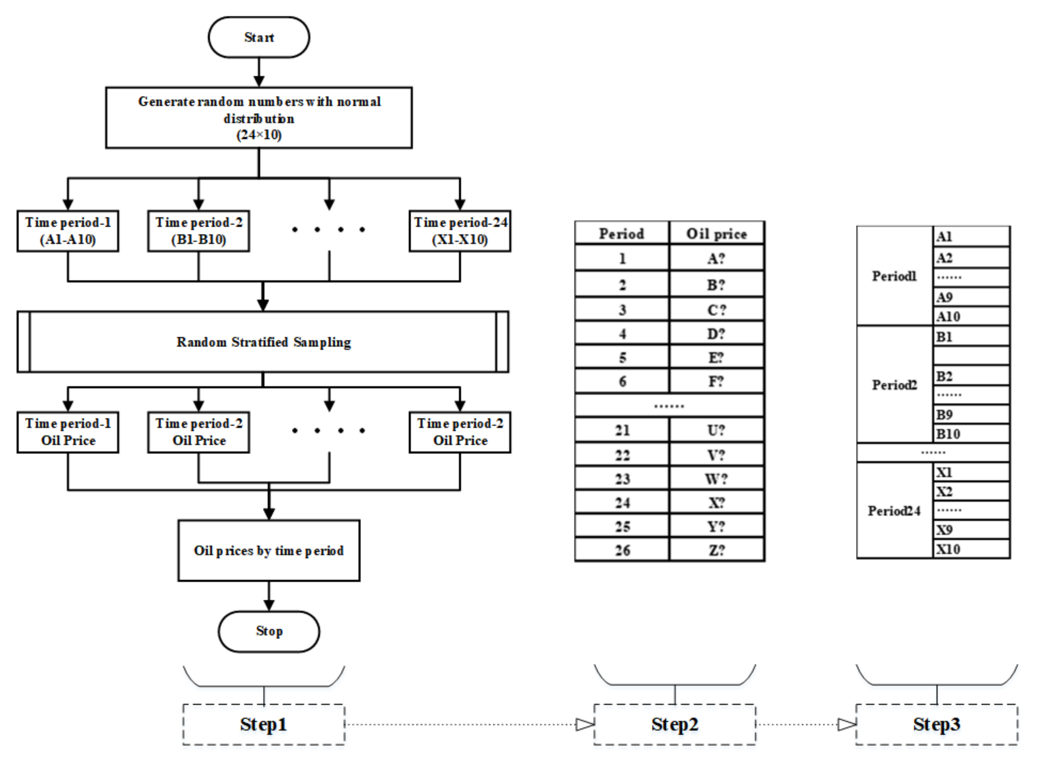
- Cost parameters: based on the method described in Figure 3, dynamic oil prices are generated, combined with the dynamic electricity prices described in the literature [33], where the high electricity price periods are 10 a.m.–8 p.m., medium electricity price periods are 6 a.m.–10 a.m. and 8 p.m.–10 p.m., and low electricity price periods are 10 p.m.–6 a.m.; dynamic costs are generated as shown in Figure 7. Other fixed costs, such as energy storage system losses, electricity load interruption, BDG unit start/stop cost are 0. 002USD, 0. 070USD, and 0. 167USD, respectively.
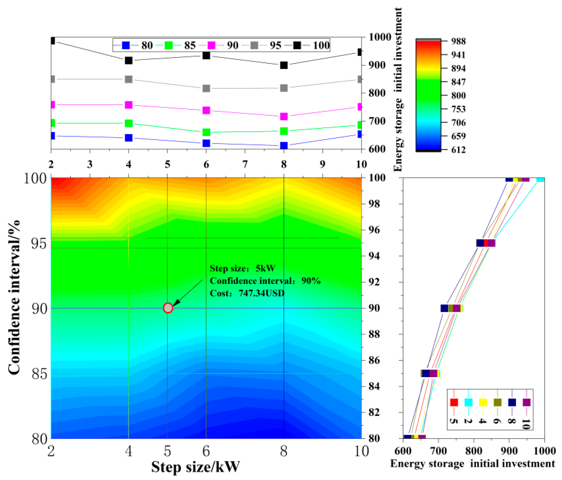
4.2. Design of Energy Storage Unit
5. Results and Analysis
5.1. Electricity and Cooling Load Demand Response
5.1.1. Electrical Load Demand Response
5.1.2. Cooling Load Demand Response
5.1.3. Evaluation of Demand Response
- a
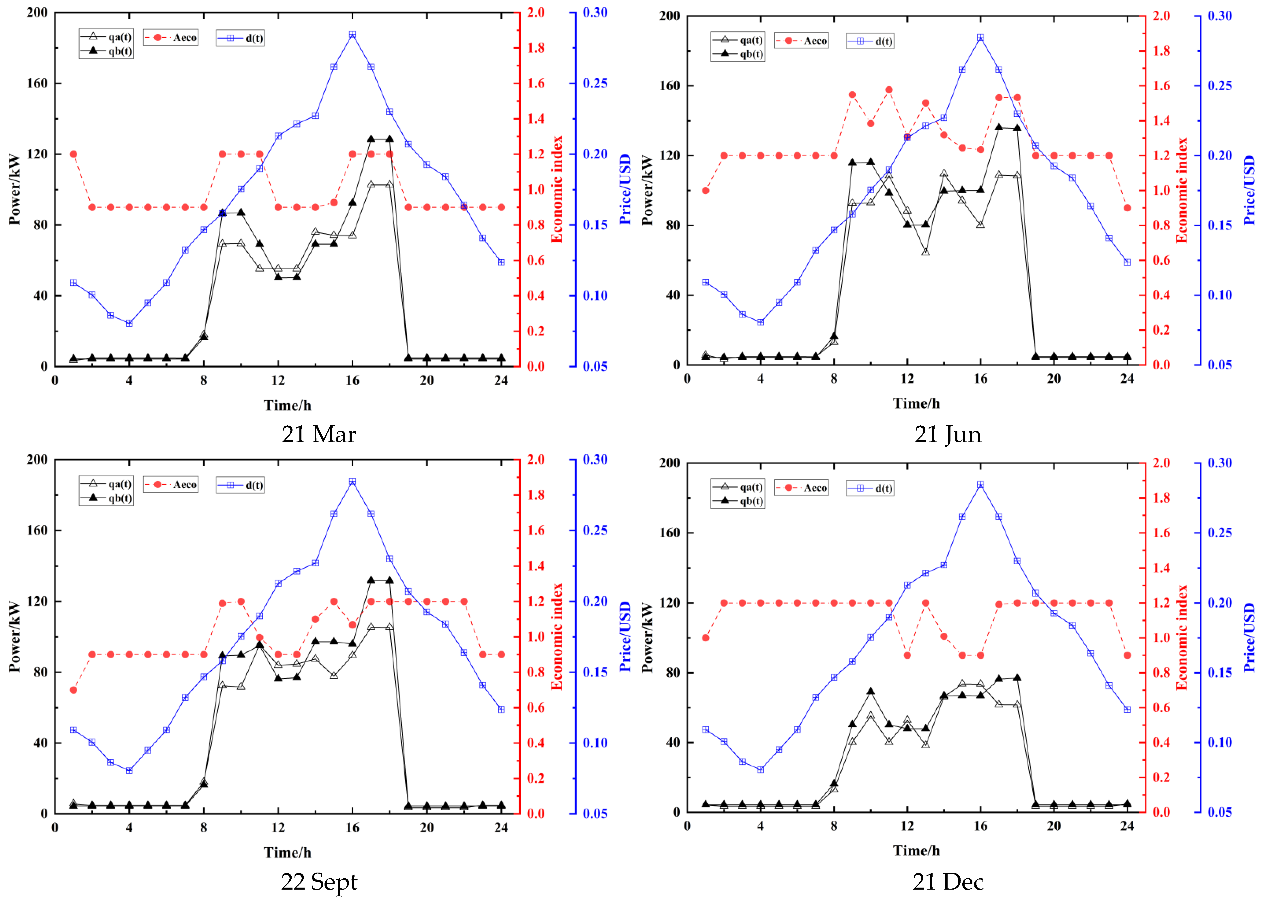
- Economic index
- b
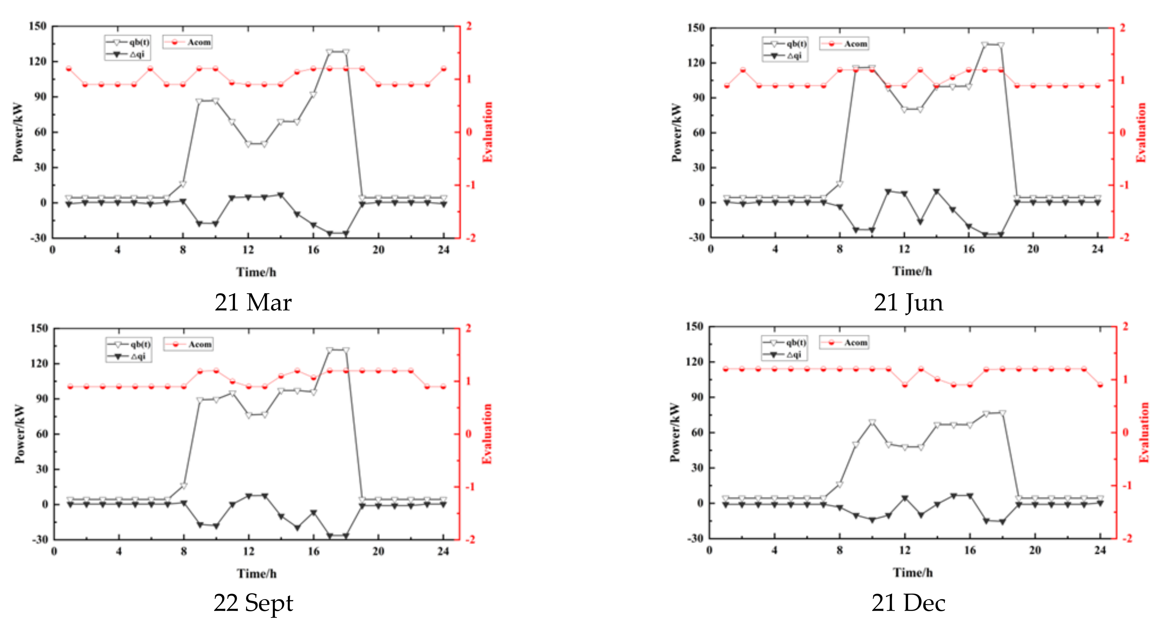
- Comfort index
5.2. Demands Scheduling Schemes
5.2.1. Scheduling Schemes for Electricity Demand
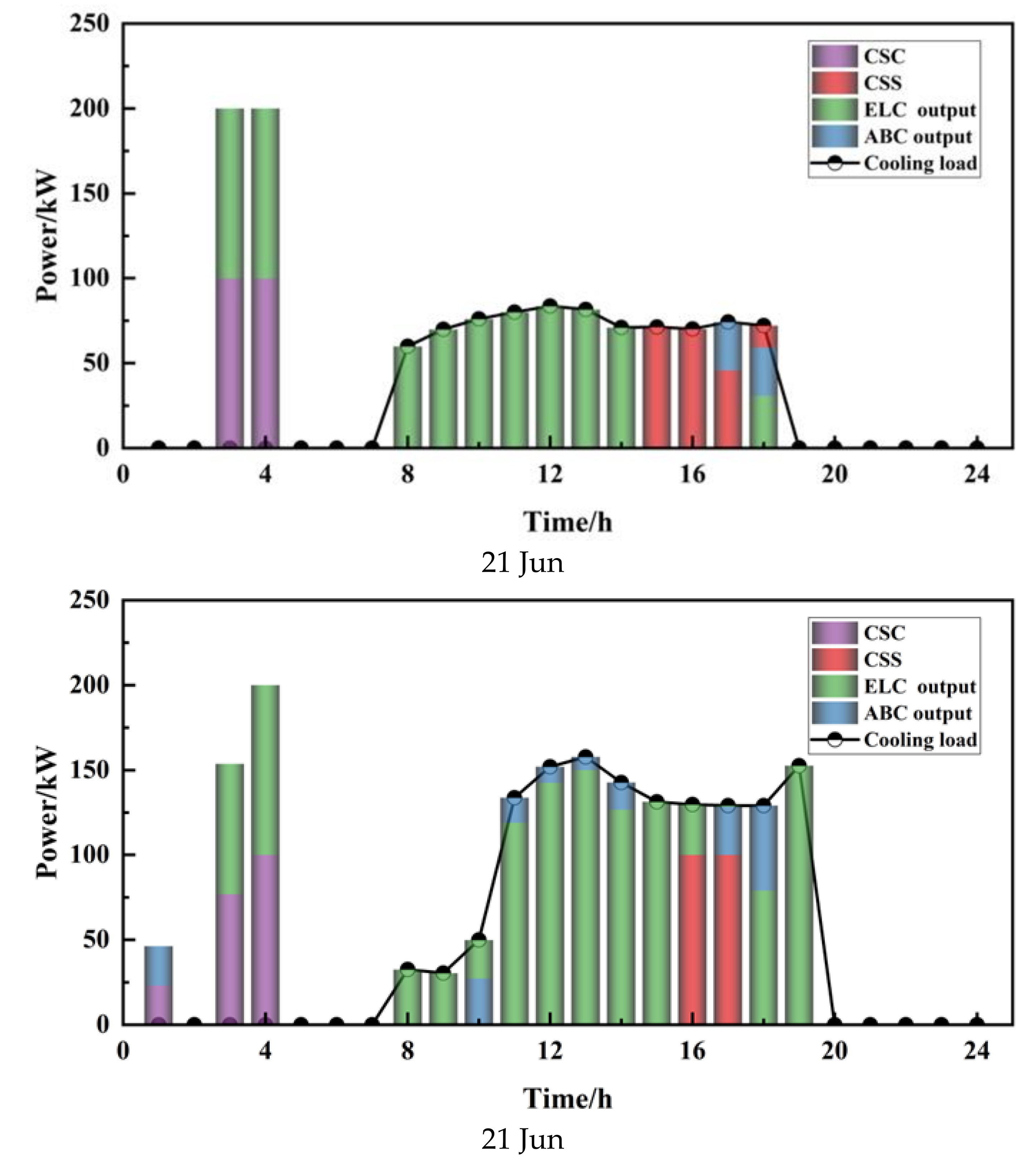
5.2.2. Scheduling Schemes for Cooling Demand
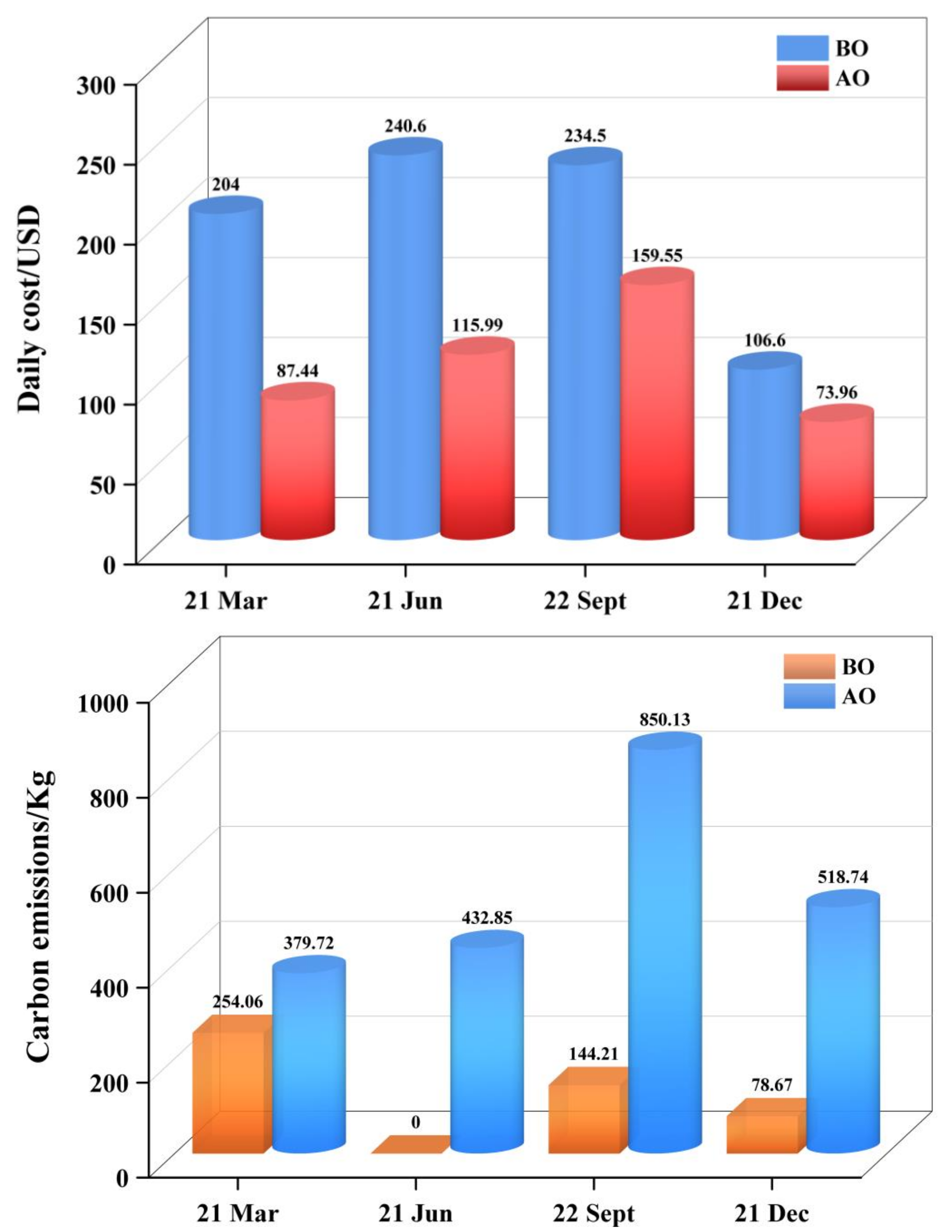
5.3. Comparison before and after Optimization
6. Conclusions
Author Contributions
Funding
Institutional Review Board Statement
Informed Consent Statement
Data Availability Statement
Conflicts of Interest
References
- Zou, C.; Xiong, B.; Xue, H.; Zheng, D.; Ge, Z.; Wang, Y.; Jiang, L.; Pan, S.; Wu, S. The role of new energy in carbon neutral. Pet. Explor. Dev. 2021, 48, 480–491. [Google Scholar] [CrossRef]
- Zhang, S.; Chen, W. China’s energy transition pathway in a carbon neutral vision. Engineering 2021, in press. [Google Scholar] [CrossRef]
- Yu, F.W.; Ho, W.T. Tactics for carbon neutral office buildings in Hong Kong. J. Clean. Prod. 2021, 326, 129369. [Google Scholar] [CrossRef]
- Zhang, S.; Wang, K.; Xu, W.; Iyer-Raniga, U.; Athienitis, A.; Ge, H.; Cho, D.W.; Feng, W.; Okumiya, M.; Yoon, G.; et al. Policy recommendations for the zero energy building promotion towards carbon neutral in Asia-Pacific Region. Energy Policy 2021, 159, 112661. [Google Scholar] [CrossRef]
- Yu, T.; Zhang, P. Economic Analysis of Reducing Photovoltaic Power Plant Abandoned Electricity by Energy Storage Based on Life Cycle Theory. Shanxi Electr. Power 2019, 4, 1–6. [Google Scholar]
- Xiao, Z.H.; Hua, X.L. A Study on the Application of Abandoned Wind Electricity in Thermal Power Plant’s Heat Recovery System. Adv. Mater. Res. 2014, 1070–1072, 343–346. [Google Scholar] [CrossRef]
- Salem, R.; Bahadori-Jahromi, A.; Mylona, A.; Godfrey, P.; Cook, D. Energy performance and cost analysis for the nZEB retrofit of a typical UK hotel. J. Build. Eng. 2020, 31, 101403. [Google Scholar] [CrossRef]
- Salem, R.; Bahadori-Jahromi, A.; Mylona, A.; Godfrey, P.; Cook, D. Investigating the potential impact of energy-efficient measures for retrofitting existing UK hotels to reach the nearly zero energy building (nZEB) standard. Energy Effic. 2019, 12, 1577–1594. [Google Scholar] [CrossRef]
- Lu, Y.; Wang, S.; Yan, C.; Huang, Z. Robust optimal design of renewable energy system in nearly/net zero energy buildings under uncertainties. Appl. Energy 2017, 187, 62–71. [Google Scholar] [CrossRef]
- Ferrara, M.; Della Santa, F.; Bilardo, M.; De Gregorio, A.; Mastropietro, A.; Fugacci, U.; Vaccarino, F.; Fabrizio, E. Design optimization of renewable energy systems for NZEBs based on deep residual learning. Renew. Energy 2021, 176, 590–605. [Google Scholar] [CrossRef]
- Borrelli, M.; Merema, B.; Ascione, F.; Francesca De Masi, R.; Peter Vanoli, G.; Breesch, H. Evaluation and optimization of the performance of the heating system in a nZEB educational building by monitoring and simulation. Energy Build. 2021, 231, 110616. [Google Scholar] [CrossRef]
- Fan, C.; Huang, G.; Sun, Y. A collaborative control optimization of grid-connected net zero energy buildings for performance improvements at building group level. Energy 2018, 164, 536–549. [Google Scholar] [CrossRef]
- Yang, J.; Su, C. Robust optimization of microgrid based on renewable distributed power generation and load demand uncertainty. Energy 2021, 223, 120043. [Google Scholar] [CrossRef]
- Jiao, F.; Ji, C.; Zou, Y.; Zhang, X. Tri-stage optimal dispatch for a microgrid in the presence of uncertainties introduced by EVs and PV. Appl. Energy 2021, 304, 117881. [Google Scholar] [CrossRef]
- Gang, W.; Wang, J.; Wang, S. Performance analysis of hybrid ground source heat pump systems based on ANN predictive control. Appl. Energy 2014, 136, 1138–1144. [Google Scholar] [CrossRef]
- Pan, I.; Das, S. Fractional order fuzzy control of hybrid power system with renewable generation using chaotic PSO. ISA Trans. 2016, 62, 19–29. [Google Scholar] [CrossRef]
- Nasri, S.; Sami, B.S.; Cherif, A. Power management strategy for hybrid autonomous power system using hydrogen storage. Int. J. Hydrog. Energy 2016, 41, 857–865. [Google Scholar] [CrossRef]
- Chu, H. Genetic algorithm-based optimal scheduling of microgrids. Ind. Control. Comput. 2019, 32, 151–153. [Google Scholar]
- Das, B.; Kumar, A. A NLP approach to optimally size an energy storage system for proper utilization of renewable energy sources. Procedia Comput. Sci. 2018, 125, 483–491. [Google Scholar] [CrossRef]
- Lu, Y.; Wang, S.; Sun, Y.; Yan, C. Optimal scheduling of buildings with energy generation and thermal energy storage under dynamic electricity pricing using mixed-integer nonlinear programming. Appl. Energy 2015, 147, 49–58. [Google Scholar] [CrossRef]
- Antonopoulos, I.; Robu, V.; Couraud, B.; Kirli, D.; Norbu, S.; Kiprakis, A.; Flynn, D.; Elizondo-Gonzalez, S.; Wattam, S. Artificial intelligence and machine learning approaches to energy demand-side response: A systematic review. Renew. Sustain. Energy Rev. 2020, 130, 109899. [Google Scholar] [CrossRef]
- Borges, N.; Soares, J.; Vale, Z. A Robust Optimization for Day-ahead Microgrid Dispatch Considering Uncertainties. IFAC-Paper 2017, 50, 3350–3355. [Google Scholar] [CrossRef]
- Chiñas-Palacios, C.; Vargas-Salgado, C.; Aguila-Leon, J.; Hurtado-Pérez, E. A cascade hybrid PSO feed-forward neural network model of a biomass gasification plant for covering the energy demand in an AC microgrid. Energy Convers. Manag. 2021, 232, 113896. [Google Scholar] [CrossRef]
- Gao, D.-C.; Sun, Y. A GA-based coordinated demand response control for building group level peak demand limiting with benefits to grid power balance. Energy Build. 2016, 110, 31–40. [Google Scholar] [CrossRef]
- Shehzad Hassan, M.A.; Chen, M.; Lin, H.; Ahmed, M.H.; Khan, M.Z.; Chughtai, G.R. Optimization modeling for dynamic price based demand response in microgrids. J. Clean. Prod. 2019, 222, 231–241. [Google Scholar] [CrossRef]
- Yang, X.; Leng, Z.; Xu, S.; Yang, C.; Yang, L.; Liu, K.; Song, Y.; Zhang, L. Multi-objective optimal scheduling for CCHP microgrids considering peak-load reduction by augmented ε-constraint method. Renew. Energy 2021, 172, 408–423. [Google Scholar] [CrossRef]
- Jin, P.; Ai, X.; Xu, J. An Economic Operation Model for Isolated Microgrid Based on Sequence Operation Theory. Proc. CSEE 2012, 32, 52–59+10. [Google Scholar]
- Li, J. China’s biomass energy development status and outlook. China Power Enterp. Manag. 2021, 1, 70–73. [Google Scholar]
- Liu, Y.; Xu, J.; Zhang, Q.; Chen, C.; Zhou, Q.; Zhou, Q. Research advance and future prospect on production of biodiesel from waste cooking oil. Chin. J. Ecol. 2021, 40, 2243–2250. [Google Scholar]
- Lu, Y.; Wang, S.; Zhao, Y.; Yan, C. Renewable energy system optimization of low/zero energy buildings using single-objective and multi-objective optimization methods. Energy Build. 2015, 89, 61–75. [Google Scholar] [CrossRef]
- Tang, W.; Gao, F. Optimal Operation of Household Microgrid Day-ahead Energy Considering User Satisfaction. High Volt. Eng. 2017, 43, 140–148. [Google Scholar]
- Li, Y.; Han, M.; Yang, Z.; Li, G. Coordinating Flexible Demand Response and Renewable Uncertainties for Scheduling of Community Integrated Energy Systems with an Electric Vehicle Charging Station: A Bi-Level Approach. IEEE Trans. Sustain. Energy 2021, 12, 2321–2331. [Google Scholar] [CrossRef]
- Jia, H.; Peng, J.; Li, N.; Zou, C.; Yin, R.; Tai, Y. Optimazation and economic analysis of distributed photovoltaic-energy storage system under dynamic electricity price. Acta Energ. Sol. Sin. 2021, 42, 187–193. [Google Scholar]
- Zhao, Y.; Lu, Y.; Yan, C.; Wang, S. MPC-based optimal scheduling of grid-connected low energy buildings with thermal energy storages. Energy Build. 2015, 86, 415–426. [Google Scholar] [CrossRef]


| Specification | ||
|---|---|---|
| Feature | Actual Value | Model Value |
| Orientation | South-east | South-east |
| Total net floor area (m2) | 1520 | 1520 |
| Window-to-wall ratio | <10–40% | <10–40% |
| Shading | 45° (angle) | 45° (angle) |
| Wall U value (W/(m2 ∗ K))/absorption | <1.0/<0.4 | <1.0/<0.4 |
| Roof U value (W/(m2 ∗ K))/absorption | <1.0/<0.3 | <1.0/<0.3 |
| Types of Renewable Energy | PV | PV/WT |
| PV (m2) | 1015 | 1015 |
| Peak output of PV (kWp) | 150 | 150 |
| WT (kW) | 0 | 50 |
| Rated power of bio-diesel generator (kW) | 100 | 100 |
| Type of chiller unit | Electric/Adsorption | Ground source heat pump/Adsorption |
| Maximum no. of people (including visitors) | 200 | 200 |
| Date | Average Value (Acom) |
|---|---|
| 21 Mar | 1.129 |
| 21 Jun | 1.002 |
| 22 Sep | 0.977 |
| 21 Dec | 0.930 |
| Date | Comparison before and after Optimization | ||
|---|---|---|---|
| Daily Cost/USD | Carbon Emission/kg | Average Daily Abandoned Power Ratio/% | |
| 21 Mar | 116.56 | −125.66 | 19.63 |
| 21 Jun | 124.61 | −432.85 | 49.14 |
| 22 Sept | 74.95 | −705.92 | 24.30 |
| 21 Dec | 32.64 | −440.07 | 52.49 |
Publisher’s Note: MDPI stays neutral with regard to jurisdictional claims in published maps and institutional affiliations. |
© 2022 by the authors. Licensee MDPI, Basel, Switzerland. This article is an open access article distributed under the terms and conditions of the Creative Commons Attribution (CC BY) license (https://creativecommons.org/licenses/by/4.0/).
Share and Cite
Lv, T.; Lu, Y.; Zhou, Y.; Liu, X.; Wang, C.; Zhang, Y.; Huang, Z.; Sun, Y. Optimal Control of Energy Systems in Net-Zero Energy Buildings Considering Dynamic Costs: A Case Study of Zero Carbon Building in Hong Kong. Sustainability 2022, 14, 3136. https://doi.org/10.3390/su14063136
Lv T, Lu Y, Zhou Y, Liu X, Wang C, Zhang Y, Huang Z, Sun Y. Optimal Control of Energy Systems in Net-Zero Energy Buildings Considering Dynamic Costs: A Case Study of Zero Carbon Building in Hong Kong. Sustainability. 2022; 14(6):3136. https://doi.org/10.3390/su14063136
Chicago/Turabian StyleLv, Tao, Yuehong Lu, Yijie Zhou, Xuemei Liu, Changlong Wang, Yang Zhang, Zhijia Huang, and Yanhong Sun. 2022. "Optimal Control of Energy Systems in Net-Zero Energy Buildings Considering Dynamic Costs: A Case Study of Zero Carbon Building in Hong Kong" Sustainability 14, no. 6: 3136. https://doi.org/10.3390/su14063136
APA StyleLv, T., Lu, Y., Zhou, Y., Liu, X., Wang, C., Zhang, Y., Huang, Z., & Sun, Y. (2022). Optimal Control of Energy Systems in Net-Zero Energy Buildings Considering Dynamic Costs: A Case Study of Zero Carbon Building in Hong Kong. Sustainability, 14(6), 3136. https://doi.org/10.3390/su14063136