Spatio-Temporal Solar–Wind Complementarity Assessment in the Province of Kalinga-Apayao, Philippines Using Canonical Correlation Analysis ^†

Abstract

Increased utilization of renewable energy (RE) resources is critical in achieving key climate goals by 2050. The intermittent nature of RE, especially solar and wind, however, poses reliability concerns to the utility grid. One way to address this problem is to harmonize the RE resources using spatio-temporal complementarity analysis. Two RE resources are said to be complementary if the lack of one is balanced by the abundance of the other, and vice versa. In this work, solar–wind complementarity was analyzed across the provinces of Kalinga and Apayao, Philippines, which are potential locations for harvesting RE as suggested by the Philippine Department of Energy. Global horizontal irradiance (GHI) and wind speed data sets were obtained from the NASA POWER database and then studied using canonical correlation analysis (CCA), a multivariate statistical technique that finds maximum correlations between time series data. We modified the standard CCA to identify pairs of locations within the region of study with the highest solar–wind complementarity. Results show that the two RE resources exhibit balancing in the resulting locations. By identifying these locations, solar and wind resources in the Philippine islands can be integrated optimally and sustainably, leading to a more stable power and increased utility grid reliability.

1. Introduction

International efforts to decarbonize using renewable energy (RE) resources are currently underway [1], leading to expanding electricity generation [2,3]. In recent years, the costs of RE have been declining, and their global investments have also continued to rise [4]. For instance, a recent review indicated that solar photovoltaics (PV) and wind turbines now contribute two-thirds to the growth of RE [2]. This trend has also inspired nations to increase their renewable energy targets as part of their low-emission development strategy.

In the case of island countries, renewable energy projects primarily focus on stand-alone systems in off-grid areas. However, stand-alone variable renewable energy (VRE) sources such as solar or wind energy pose flexibility and reliability challenges in meeting demand [5], since their output profiles are intermittent [6]. Possible solutions to these issues include grid expansion, grid upgrades, or increased energy storage [7]. A better way to address the problem is to harmonize the power output from two or more VREs by measuring their complementarity. More specifically, two RE resources are complementary if one resource is high when the other is low, and vice versa, in a specific region [6,8,9]. In other words, the lack of one resource is balanced by the abundance of the other at multiple different points in time [10,11]. If two or more VRE resources are harvested at locations with optimal complementarity, then off-grid areas can be provided with more stable power [11], despite having intermittent output profiles from each VRE resource. Moreover, it can help reduce the need for energy storage in the area, which usually accounts for a big share in the initial capital expenditure [10].

In an extensive review of the complementarity of renewable energy sources, it was identified that most studies focus on systems that combine solar and wind energy [12]. An optimized complementarity between solar and wind can achieve up to 30% grid penetration without adding storage [13]. Some of these assessments were conducted by identifying optimum locations with the highest potential for solar–wind installations, such as [14] for Rio Grande do Sil, Brazil and [15] for the Iberian Peninsula. In Italy, Monforti et al. [16] observed national and regional complementarity for solar and wind, supporting their energy system integration. Cao et al. [17] also evaluated the solar–wind complementarity in Shandong province, China and even provided analyses at multiple time scales. Unlike these studies, the complementarity between three REs, namely solar, wind, and tidal, were also investigated by Neto et al. [18] in Maranhao, Brazil. In addition, another study in Brazil proposed to use factor analysis to group together locations with similar RE profiles first, before evaluating solar–wind–hydro complementarity [19]. Meanwhile, some studies focused on the complementarity assessment of a single RE source only, such as the analysis of solar PV outputs on Reunion Island [20].

To quantify the degree of complementarity between two RE sources, many complementarity indices can be used [21]. Typical complementarity indices involve the analysis of anti-correlation between pairwise RE resource time series data [12]. A few examples of these indices include the Pearson correlation, Kendall correlation, and Spearman’s rank correlation coefficients [12]. For instance, if the output profiles of two REs are anti-correlated, then their Pearson correlation coefficient is negative. The more negative the Pearson coefficient, the better the complementarity [12]. A different perspective was recently proposed by Berger et al. [22], which uses the concept of critical time windows rather than correlation analysis. In that paper, two energy plants are said to be complementary if they have a minimum total likelihood of critically low production events.

Most energy complementarity studies still rely on correlation indices such as the Pearson correlation. However, these indices are not suitable for simultaneously assessing spatial and temporal energy complementarity. According to Jurasz et al. [12], there are three different ways to analyze energy complementarity: temporal, spatial, and spatio-temporal (see Figure 1). A temporal analysis only assesses the complementarity of two REs in a single location as they balance each other through time. A spatial analysis considers the average output of two REs over a period of time at multiple locations in space, then finds which areas have the most complementary REs. In contrast, a spatio-temporal analysis considers both the temporal and spatial variation of two REs, then finds locations with the best complementarity. In this case, multivariate statistical techniques should be used to comprehensively analyze time series data across multiple locations at once [11].

This work aims to identify specific sites within the Philippine provinces of Kalinga and Apayao where solar–wind spatio-temporal complementarity is optimal using advanced multivariate statistical techniques. This region is chosen following a report [23] that classifies these provinces to have high-quality RE resources with commercial interest. This paper proposes a modified canonical correlation analysis (CCA) method to assess solar–wind complementarity across multiple locations in the Kalinga-Apayao region. The original CCA method was already explored for solar–wind complementarity analysis by Santos-Alamillos et al. [11]. The goal of CCA is to find maximally correlated associations between two multivariate data sets. These associations, known as the canonical variates, are expressed as linearly weighted combinations of the input variables. CCA derives the weights so that the canonical variates have a maximum correlation. Because of this capability, CCA can be performed between the solar and wind data sets to find maximally anti-correlated scores, since anti-correlation translates to good complementarity [11]. In this work, we also propose to compute a CCA complementarity matrix to conveniently present the information extracted from the CCA weights.

Our work demonstrates that the proposed CCA provides better interpretability and computational efficiency, while still giving consistent results with other techniques such as the Pearson correlation and the CIWS (complementarity index of wind and solar radiation) metric by Li et al. [24]. The results of this work can have a significant impact on the Philippine energy planning, as it provides insights to energy developers and investors by identifying suitable locations for future solar and wind projects in the islands.

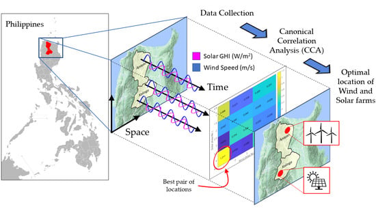
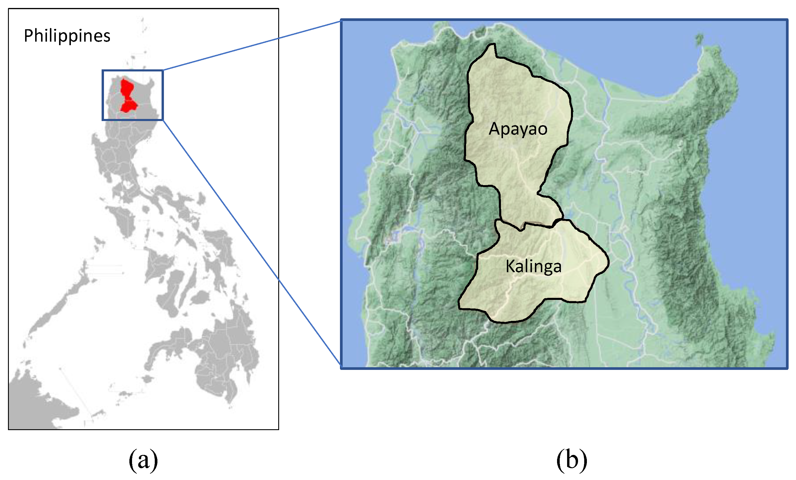
2. Materials and Methods

2.1. Data Collection and Pre-Processing

Apayao and Kalinga are part of the Cordillera Administrative Region of the Philippines which can be found north of the country as shown in Figure 2a. Kalinga, a land-locked province, has a land area of 3164.3 km² [25]. It is characterized by mountainous terrain whose peaks range from 1500 m to 2500 m. The other location, Apayao, can be found north of Kalinga. It is bigger than Kalinga having a land area of 5113 km² [25]. Based on its geographic features, Apayao is segmented into Upper Apayao and Lower Apayao. Upper Apayao is characterized by mountain ranges with valleys in between, whereas Lower Apayao has flat mountains and plateaus [25]. Both locations experience an interchanging wet and dry season per year.

Two kinds of data sets were retrieved from the NASA POWER database [26] across the Kalinga-Apayao provincial area, namely: (a) the daily all-sky downward short-wave irradiance (kWh/m²/day); and (b) the daily wind speed (m/s) at 10 m and 50 m from sea level. The data span the period from 1 January 2000 to 31 December 2020, translating to a total of 7671 values for each time series. The downward short-wave irradiance, which is representative of the global horizontal irradiance (GHI), quantifies the solar energy resources of the locations. Note that the all-sky irradiance values were selected rather than the clear-sky values to consider cloud cover. Before further analysis, the GHI values were converted to a more common unit of W/m². Meanwhile, the wind speeds at 10 m and 50 m were used to determine the surface roughness exponent, α, through calibration via the following equation [11],

$$\frac{V_1}{V_0}={\left(\frac{H_1}{H_0}\right)}^{\alpha },$$

(1)

where $V_0$ and $V_1$ are the wind speeds at $H_0=10 \mathrm{m}$ and $H_1=50$ m hub heights, respectively. The wind speed values were adjusted to a more appropriate hub height of 100 m using the same Equation (1), as suggested by Heide et al. [27].

Initially, the spatial resolution for downloading the data sets in the Kalinga-Apayao region was set by dividing it into 5.9 km by 5.9 km cells. The initial data set contains GHI and wind speed values at the center of each of the 250 cells, as depicted in Figure 3. However, upon inspecting the downloaded data from NASA POWER, it was observed that there were only four areas with unique GHI values and five areas with unique wind speed values in the entire region. Figure 3a labels the cells that share the exact same GHI data with the same color, whereas Figure 3b labels those that share the exact same wind speed data with the same color. Hence, these composite areas were assigned to be the candidate locations for harvesting solar and wind energy. For the rest of the paper, we use the labels Area S1, S2, …, S4 for solar and Area W1, W2, …, W5 for wind area candidates.

2.2. Canonical Correlation Analysis

Canonical Correlation Analysis (CCA) is a multivariate statistical technique, initially proposed by Hotelling in 1936 [28], to find maximum correlations between any two sets of data. In this study, the two data sets are the GHI and wind speed. The CCA algorithm in this work is based on a similar CCA algorithm used in control systems engineering [29]. In the following text, we modified the original CCA so that it can output the pair of areas where solar–wind complementarity is highest.

Let ${\mathit{X}}_a\in {\Re }^{N\times M_a}$ and ${\mathit{X}}_b\in {\Re }^{N\times M_b}$ denote the GHI (W/m²) and wind speed (m/s) data, respectively, where $N$ is the total number of time steps and $M_a$, $M_b$ are the number of candidate geographical areas for solar and wind harvesting, respectively. The data is first normalized to zero-mean and unit-variance in each geographical area (column), so that the effects of differing scales and biases are removed from the analysis. That is, the mean of each signal is removed from the signal, and then the zero-mean signals are scaled by dividing with their respective variances. Next, the signs of ${\mathit{X}}_a$ (or equivalently, ${\mathit{X}}_b$) are flipped, that is, ${\mathit{X}}_a≔-{\mathit{X}}_a$, to let CCA maximize anti-correlations rather than correlations. We assume that two time series with higher anti-correlation translates to better complementarity [13].

The covariance and cross-covariances of ${\mathit{X}}_a$ and ${\mathit{X}}_b$ can be computed as [29],

$${\Sigma }_{aa}={\mathit{X}}_a^T{\mathit{X}}_a/\left(N-1\right)$$

(2)

$${\Sigma }_{bb}={\mathit{X}}_b^T{\mathit{X}}_b/\left(N-1\right)$$

(3)

$${\Sigma }_{ab}={\mathit{X}}_a^T{\mathit{X}}_b/\left(N-1\right).$$

(4)

Mathematically, CCA aims to find weights ${\mathit{w}}_a\in {\Re }^{M_a} \mathrm{and} {\mathit{w}}_b\in {\Re }^{M_b}$ so that the correlation $\rho$ between the transformed data ${\mathit{X}}_a{\mathit{w}}_a$ and ${\mathit{X}}_b{\mathit{w}}_b$ is maximum [29]. This correlation can be computed as,

$$\rho =\frac{{\mathit{w}}_a^T{\Sigma }_{ab}{\mathit{w}}_b}{{\left({\mathit{w}}_a^T{\Sigma }_{aa}{\mathit{w}}_a\right)}^{1/2}{\left({\mathit{w}}_b^T{\Sigma }_{bb}{\mathit{w}}_b\right)}^{1/2}},$$

(5)

which can be re-written into the following maximization problem [29],

$$\begin{gathered} \underset{u, v}{\max } \rho ={\mathit{u}}^T\left({\Sigma }_{aa}^{-1/2}{\Sigma }_{ab}{\Sigma }_{bb}^{-1/2}\right)\mathit{v}, \\ s.t. {\mathit{u}}^T\mathit{u}=1, {\mathit{v}}^T\mathit{v}=1 \end{gathered}$$

(6)

by defining $\mathit{u}={\Sigma }_{aa}^{1/2} {\mathit{w}}_a$ and $\mathit{v}={\Sigma }_{bb}^{1/2} {\mathit{w}}_b$ as the scaled weight vectors. According to [28], the solution to Equation (6) is given by the singular value decomposition (SVD) of the Hankel matrix $\mathit{H}$ as follows,

$$\mathit{H}={\Sigma }_{aa}^{-1/2}{\Sigma }_{ab}{\Sigma }_{bb}^{-1/2}=\mathit{U}\Sigma {\mathit{V}}^T,$$

(7)

where $\mathit{U}=\left[{\mathit{u}}_1,{\mathit{u}}_2,\dots ,{\mathit{u}}_r\right]$ and $\mathit{V}=\left[{\mathit{v}}_1,{\mathit{v}}_2,\dots ,{\mathit{v}}_r\right]$ are matrices containing the left and right singular vectors, respectively, $\mathit{\Sigma }=\mathrm{diag}\left({\sigma }_1,{\sigma }_2,\dots ,{\sigma }_r\right)$ is the diagonal matrix of descending singular values, and $r$ is the rank of $\mathit{H}$ [29].

To find the most correlated pair of time series, only the first canonical mode is important, that is, the tuple $\left({\mathit{u}}_1,{\mathit{v}}_1,{\sigma }_1\right)$. The first singular value ${\sigma }_1$ is the value of the maximum correlation $\rho$ from Equation (5). Meanwhile, the weights are recovered from the singular vectors as ${\mathit{w}}_a={\Sigma }_{aa}^{-1/2}{\mathit{u}}_1$ and ${\mathit{w}}_b={\Sigma }_{bb}^{-1/2}{\mathit{v}}_1$.

The weights ${\mathit{w}}_a$, ${\mathit{w}}_b$ contain valuable information as to which pair of geographical areas possess the best spatio-temporal solar–wind complementarity. Note that ${\mathit{w}}_a$ and ${\mathit{w}}_b$ are both column vectors containing $M_a$ and $M_b$ elements, respectively. Each element can be interpreted as the amount of contribution given by the time series data from each geographical area that goes into maximizing the correlation in Equation (5). Therefore, the pair of locations (one from solar data ${\mathit{w}}_a$ and one from wind data ${\mathit{w}}_b$) with the largest contributions of the same sign has the best solar–wind complementarity among all possible pairs of locations. To put this notion mathematically, we take the additional step of computing the following outer product, which we call the CCA complementarity matrix,

$$\mathit{C}={\mathit{w}}_a{\mathit{w}}_b^T\in {\Re }^{M_a\times M_b},$$

(8)

and then find the ith row and jth column where the maximum of all elements of $\mathit{C}$ is located. The result signifies that the GHI data from Area i is best complemented by the wind speed data from Area j. To obtain a ranking of the next best pairs of locations, the next highest elements of matrix $\mathit{C}$ are taken in descending order.

Arguably, the traditional way of generating a complementarity matrix in Equation (8) is to compute the pairwise Pearson correlation coefficient between the solar and wind time series data from multiple locations. It produces a similar result as to which two individual time series are most anti-correlated, which corresponds to the two locations where solar–wind complementarity is best. However, we note that the Pearson correlation analysis can only evaluate one-to-one associations between two variables, whereas CCA can evaluate many-to-many associations between two sets of multiple variables. In one step, CCA can already compute which set of locations for solar have the most anti-correlated data with which set of locations for wind (this information is contained in the weights ${\mathit{w}}_a$ and ${\mathit{w}}_b$). In contrast, the Pearson correlation needs to iterate on every possible solar–wind pair of locations to check for the best complementarity. Hence, CCA is more suitable for multivariate data analysis, such as in spatio-temporal complementarity assessment. Moreover, at the core of CCA is the maximization of precisely the Pearson correlation coefficient in Equations (6) and (7). This means that the results of the proposed CCA from Equation (8) and that of the pairwise Pearson correlation analysis are expected to agree to some extent. In Section 3.2 of this paper, we demonstrate empirically that this is indeed the case.

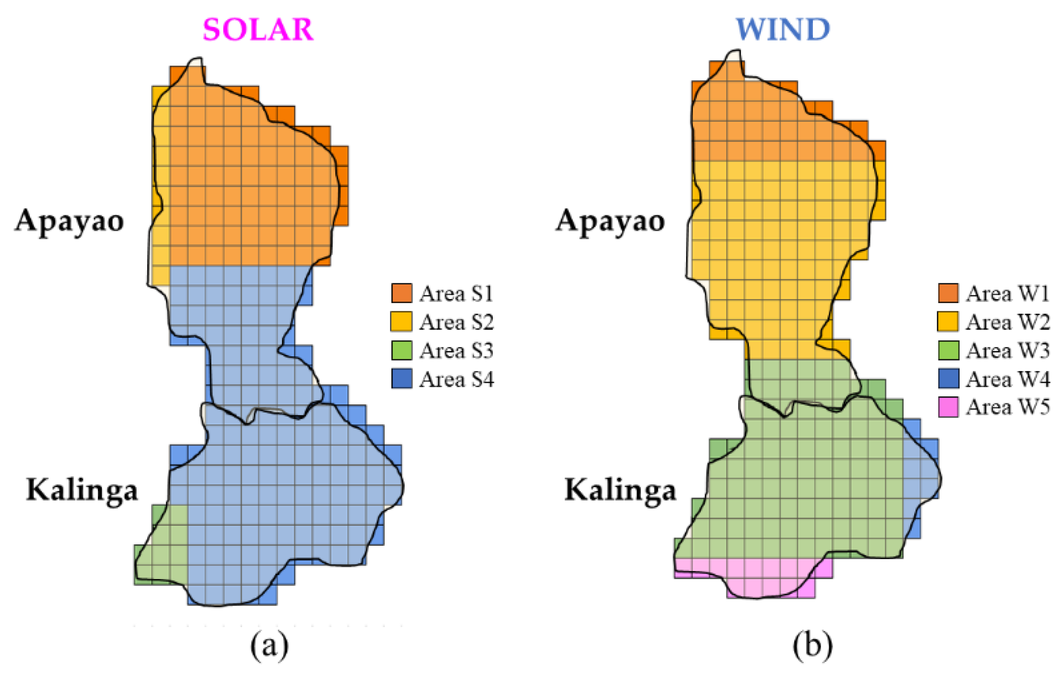
3. Results and Discussion

3.1. Solar–Wind Complementarity Analysis

The data set obtained from the NASA POWER database was normalized to zero-mean and unit-variance prior to any analysis. This means that the respective means of each solar GHI and wind speed time series were removed from each signal, and then the resulting time series were divided by their respective variances. As mentioned in Section 2.2, this pre-processing step is performed to remove the influence of differing scales and biases from the complementarity assessment.

The normalized time series are now presented in Figure 4. The most apparent trend in the data is seasonality, that is, periods of high and low values of each signal alternating across time. Solar GHI values are typically high from March to September, and low in the other months. These months can be attributed to the hot and cold seasons of the country, respectively. Meanwhile, wind speed values are low from April to July and high in the other months. Although these trends already show promising periods where solar and wind resources are complementary, this paper aims to find the exact pair of areas where complementarity is highest using CCA.

Using CCA, the singular values obtained from Equation (7) were analyzed first from the normalized time series (see Figure 5). The maximum correlation was found to be ${\sigma }_1=0.7455$ for the first canonical mode. This number denotes the maximum extent of complementarity between the canonical variates, i.e., the weighted combination of solar sources and the weighted combination of wind sources within the Kalinga-Apayao region. Note that a perfect complementarity would give ${\sigma }_1=1.00$, in which case there is a certain combination of solar sources that exactly complements a certain combination of wind sources. Meanwhile, the third and fourth canonical modes are not helpful in elucidating energy complementarity in the region since their corresponding singular values are too low (see Figure 5).

Upon inspecting the weights ${\mathit{w}}_a$ and ${\mathit{w}}_b$ from the first canonical mode, the CCA complementarity matrix was computed (see Equation (8)). As shown in Figure 6a, the pair of areas within Kalinga-Apayao that are best for energy harvesting is Solar Area 4 and Wind Area 1. From here on, we use the notation Si-Wj to denote location pairs: Solar Area i and Wind Area j. Hence, the best pairs of locations are S4-W1. This pairing achieved a score of ${\mathit{C}}_{ij}=1.217$, having a large margin of increase from the score of the next best pair, S1-W1, whose score is ${\mathit{C}}_{ij}=0.698$. To verify this result, the normalized GHI and wind speed time series from the pair S4-W1 is shown in Figure 7a, showing that the two time series are indeed balancing each other around the mean. Periods of high GHI values can be attributed to the dry season in the country, typically from March to August every year. The periods of high wind speeds are found during the wet season, from June to December. Note that the dry and wet seasons are the only two major seasons in the country.

Although the same trends can be seen in the pair of locations with the worst complementarity (see Figure 7b for the time series from S3-W1), the balancing effect is not as apparent. For instance, in the shaded portion of the time series in Figure 7b, the GHI values from Area 3 (solid) and the wind speed from Area 1 (dashed) are too close to each other. In contrast, for the same period in Figure 7a, the GHI from Area 4 (solid) and the wind speed from Area 1 (dashed) have a much more pronounced gap. This indicates that, for S4-W1, the lack of wind resources can be balanced by the solar resource and vice versa.

3.2. Comparison of CCA to Other Approaches

Aside from the proposed CCA, this work also assessed the solar–wind complementarity in the Kalinga-Apayao region using two other approaches: (a) Pearson correlation [13]; and (b) CIWS [24]. The Pearson correlation can be computed between any two time series, such that the most anti-correlated ones (most negative correlation) represent the best complementarity. Meanwhile, CIWS computes the area of the gap between the GHI and wind speed time series. A larger gap area corresponds to better complementarity. Both the Pearson correlation and the CIWS require computation of the index for each pair of locations. This means that the algorithm must iterate on all possible pairs. In contrast, the CCA method only requires matrix computations (i.e., Equations (2)–(4)) and a singular value decomposition (i.e., Equation (7)) to output the same results. Hence, CCA requires less computation and is more suitable for simultaneously assessing complementarity between a larger number of locations.

Figure 6b,c show results from the Pearson correlation and the CIWS approach, respectively. Evidently, the results from both approaches are consistent with that of the proposed CCA in reporting S4-W1 as the pair of locations with the highest solar–wind complementarity. This means that the proposed CCA is an effective and reliable technique for complementarity analysis. As a further comparison, the top 5 pairs of locations elucidated by all three approaches are summarized in

Table 1. Ranking of best solar–wind complementary areas from 3 different methods.

Rank	Proposed CCA	Pearson Correlation	CIWS
1	S4-W1 *	S4-W1	S4-W1
2	S1-W1	S1-W1	S1-W1
3	S4-W5	S4-W2	S4-W2
4	S4-W4	S4-W4	S1-W2
5	S3-W3	S4-W3	S4-W4

* Bold entries denote results that are consistent for all methods.

. A consensus is also reached for S1-W1 as the next best pair of complementary locations. With these rankings, multiple options can be provided for planning future solar and wind projects within the Kalinga-Apayao region of the Philippines.

3.3. Consistency of Results

Now that the pair of locations with the best complementarity is known to be S4-W1 within the Kalinga-Apayao region, we finally investigate the consistency of this result by computing the Pearson correlation coefficient between the solar and wind data for each pair of locations per year. Then, the top five pairs with the most negative coefficients (most anti-correlated) are ranked for each year, as shown in Figure 8. The figure shows that the S4-W1 pairing consistently ranks the highest in complementarity every year from 2001 to 2020. In addition, the S1-W1 pairing is consistently ranked the next best pair from 2009 to 2020. The results in Figure 8 agree with the overall ranking presented in Table 1, which was computed by the proposed CCA. Hence, it can be expected to some degree that the best location, S4-W1, will remain the best for the years to come.

As a further check on the solar–wind complementarity, the monthly values of the Pearson correlation coefficient were computed for the best location pair, S4-W1, identified by the proposed CCA (see Figure 9). As mentioned, negative correlation values are more favorable since they indicate that the solar and wind time series complement each other. As seen in Figure 9 (top), most of the monthly correlation values were negative (lie below zero) for S4-W1. There were only 16 out of 252 months from 2000 to 2020 when the solar–wind correlation became positive (red dots). This means that in those 16 months, the solar and wind energy failed to complement each other for the S4-W1 locations, despite knowing that they have the best complementarity. We found that these months mainly occur from April to June every year. In the Philippines, the months from April to June are when the dry season occurs. The data shows that both solar and wind energy are typically high for these months. Hence, although these months show little complementarity, there is an immense opportunity to utilize storage systems. The addition of battery systems into our analysis is left for future work.

In contrast, the pair with the worst complementarity, namely S3-W1, has more months when the solar–wind correlation is positive. As shown in Figure 9 (bottom), there are a total of 49 out of 252 months from January 2000 to December 2020 when the solar and wind resources fail to complement each other. This number is three times worse than the one obtained from the locations with the best complementarity (Figure 9, top). Hence, it does not make sense to build solar and wind farms on S3-W1. This finding further emphasizes the impact of studying energy complementarity to find optimal locations for future wind and solar farms.

4. Conclusions

This paper assessed the solar–wind energy complementarity in the Kalinga-Apayao region of the Philippines using a modified canonical correlation analysis (CCA) algorithm. Among four candidate areas for solar PV and five candidate areas for wind farms, the pair of locations with the best spatio-temporal complementarity was determined. These results are based on analyzing the energy resource data collected from the NASA POWER database, consisting of the daily GHI and wind speed values spanning the last 20 years over the region. Furthermore, the CCA results were found to be consistent with other methods such as the Pearson correlation and the CIWS index. Hence, the solar–wind complementarity assessment in this work can contribute to the increased reliability and stability of utility grids in the Kalinga-Apayao region.

In the future, the results of this work can be further verified via techno-economic energy systems modeling upon assigning solar PV and wind farms to the chosen candidate locations. Furthermore, the scope can also be increased to include more energy sources such as hydroelectric power into the complementarity analysis. Finally, the effect of adding energy storage and variations in load demand should be taken into account in future work.

References

1. Jeong, J.; Ko, H. Bracing for Climate Impact: Renewables as a Climate Change Adaptation Strategy. Abu Dhabi, 2021. Available online: https://www.irena.org/-/media/Files/IRENA/Agency/Publication/2021/Aug/IRENA_Bracing_for_climate_impact_2021.pdf (accessed on 16 August 2021).
2. International Energy Agency (IEA). Global Energy Review 2021. 2021. Available online: https://iea.blob.core.windows.net/assets/d0031107-401d-4a2f-a48b-9eed19457335/GlobalEnergyReview2021.pdf (accessed on 16 August 2021).
3. IRENA. World Energy Transitions Outlook: 1.5 °C Pathway. Abu Dhabi, 2021. Available online: https://www.irena.org/-/media/Files/IRENA/Agency/Publication/2021/Jun/IRENA_World_Energy_Transitions_Outlook_2021.pdf (accessed on 16 August 2021).
4. Bloomberg NEF. Energy Transition Investment Trends 2021. Technical Report. 2021. Available online: https://assets.bbhub.io/professional/sites/24/Energy-Transition-Investment-Trends_Free-Summary_Jan2021.pdf. (accessed on 16 August 2021).
5. Katz, J.; Denholm, P. Using Wind and Solar to Reliably Meet Electricity Demand Greening the Grid Leveraging Renewable Energy to Achieve Long-Term Adequacy. National Renewable Energy Laboratory, 2015. Available online: https://www.nrel.gov/docs/fy15osti/63038.pdf (accessed on 16 August 2021).
6. Solomon, A.A.; Child, M.; Caldera, U.; Breyer, C. Exploiting wind-solar resource complementarity to reduce energy storage need. AIMS Energy 2020, 8, 749–770. [Google Scholar] [CrossRef]
7. Katz, J.; Cochran, J. Integrating Variable Renewable Energy into The Grid: Key Issues. National Renewable Energy Laboratory. 2015. Available online: https://www.nrel.gov/docs/fy15osti/63033.pdf (accessed on 16 August 2021).
8. Sun, W.; Harrison, G.P. Wind-solar complementarity and effective use of distribution network capacity. Appl. Energy 2019, 247, 89–101. [Google Scholar] [CrossRef] [Green Version]
9. Hoicka, C.; Rowlands, I.H. Solar and wind resource complementarity: Advancing options for renewable electricity integration in Ontario, Canada. Renew. Energy 2011, 36, 97–107. [Google Scholar] [CrossRef]
10. Solomon, A.; Kammen, D.M.; Callaway, D. Investigating the impact of wind–solar complementarities on energy storage requirement and the corresponding supply reliability criteria. Appl. Energy 2016, 168, 130–145. [Google Scholar] [CrossRef] [Green Version]
11. Santos-Alamillos, F.; Pozo-Vazquez, D.; Ruiz-Arias, J.A.; von Bremen, L.; Tovar-Pescador, J. Combining wind farms with concentrating solar plants to provide stable renewable power. Renew. Energy 2015, 76, 539–550. [Google Scholar] [CrossRef]
12. Jurasz, J.; Canales, F.A.; Kies, A.; Guezgouz, M.; Beluco, A. A review on the complementarity of renewable energy sources: Concept, metrics, application and future research directions. Sol. Energy 2020, 195, 703–724. [Google Scholar] [CrossRef]
13. Nikolakakis, T.; Fthenakis, V. The optimum mix of electricity from wind- and solar-sources in conventional power systems: Evaluating the case for New York State. Energy Policy 2011, 39, 6972–6980. [Google Scholar] [CrossRef]
14. Pianezzola, G.; Krenzinger, A.; Canales, F.A. Complementarity Maps of Wind and Solar Energy Resources for Rio Grande do Sul, Brazil. Energy Power Eng. 2017, 09, 489–504. [Google Scholar] [CrossRef] [Green Version]
15. Jerez, S.; Trigo, R.; Sarsa, A.; Plazas, R.L.; Pozo-Vazquez, D.; Montavez, J.P. Spatio-temporal Complementarity between Solar and Wind Power in the Iberian Peninsula. Energy Procedia 2013, 40, 48–57. [Google Scholar] [CrossRef] [Green Version]
16. Monforti, F.; Huld, T.; Bódis, K.; Vitali, L.; D’Isidoro, M.; Arántegui, R.L. Assessing complementarity of wind and solar resources for energy production in Italy. A Monte Carlo approach. Renew. Energy 2014, 63, 576–586. [Google Scholar] [CrossRef]
17. Cao, Y.; Zhang, Y.; Zhang, H.; Zhang, P. Complementarity assessment of wind-solar energy sources in Shandong province based on NASA. J. Eng. 2019, 2019, 4996–5000. [Google Scholar] [CrossRef]
18. Neto, P.B.L.; Saavedra, O.R.; Oliveira, D.Q. The effect of complementarity between solar, wind and tidal energy in isolated hybrid microgrids. Renew. Energy 2020, 147, 339–355. [Google Scholar] [CrossRef]
19. Rosa, C.D.O.C.S.; Christo, E.D.S.; Costa, K.A.; dos Santos, L. Assessing complementarity and optimising the combination of intermittent renewable energy sources using ground measurements. J. Clean. Prod. 2020, 258, 120946. [Google Scholar] [CrossRef]
20. David, M.; Andriamasomanana, F.H.R.; Liandrat, O. Spatial and Temporal Variability of PV Output in an Insular Grid: Case of Reunion Island. Energy Procedia 2014, 57, 1275–1282. [Google Scholar] [CrossRef]
21. Jurasz, J.; Beluco, A.; Canales, F.A. The impact of complementarity on power supply reliability of small scale hybrid energy systems. Energy 2018, 161, 737–743. [Google Scholar] [CrossRef]
22. Berger, M.; Radu, D.; Fonteneau, R.; Henry, R.; Glavic, M.; Fettweis, X.; Le Du, M.; Panciatici, P.; Balea, L.; Ernst, D. Critical time windows for renewable resource complementarity assessment. Energy 2020, 198, 117308. [Google Scholar] [CrossRef] [Green Version]
23. Lee, N.; Dyreson, A.; Hurlbut, D.; McCan, M.I.; Neri, E.V.; Reyes, N.C.R.; Capongcol, M.C.; Cubangbang, H.M.; Agustin, B.P.Q.; Bagsik, J.; et al. Ready for Renewables: Grid Planning and Competitive Renewable Energy Zones (CREZ) in the Philippines. 2020. Available online: https://www.nrel.gov/docs/fy20osti/76235.pdf (accessed on 16 August 2021).
24. Li, W.; Stadler, S.; Ramakumar, R. Modeling and assessment of wind and insolation resources with a focus on their complementary nature: A case study of Oklahoma. Ann. Assoc. Am. Geogr. 2011, 101, 717–729. [Google Scholar] [CrossRef]
25. Philippine Statistics Authority. Cordillera Administrative Region. 2020. Available online: http://rssocar.psa.gov.ph/kalinga (accessed on 16 August 2021).
26. Stackhouse, P.W., Jr.; Macpherson, B.; Broddle, M.; McNeil, C.; Barnett, J.; Mikovitz, C.; Zhang, T. NASA Prediction of Worldwide Energy Resources (POWER) Project. 2021. Available online: https://power.larc.nasa.gov/ (accessed on 16 August 2021).
27. Heide, D.; von Bremen, L.; Greiner, M.; Hoffmann, C.; Speckmann, M.; Bofinger, S. Seasonal optimal mix of wind and solar power in a future, highly renewable Europe. Renew. Energy 2010, 35, 2483–2489. [Google Scholar] [CrossRef]
28. Hotelling, H. Relations between Two Sets of Variates. Biometrika 1936, 28, 321–377. [Google Scholar] [CrossRef]
29. Pilario, K.E.S.; Cao, Y.; Shafiee, M. A Kernel Design Approach to Improve Kernel Subspace Identification. IEEE Trans. Ind. Electron. 2020, 68, 6171–6180. [Google Scholar] [CrossRef]
Figure 1. Different types of complementarity analysis in literature: (a) temporal; (b) spatial; and (c) spatio-temporal complementarity (this study).
Sustainability 14 03253 g001
Figure 2. (a) Map of the Philippines; (b) Map of the Kalinga-Apayao Province (Coordinates: 17.243, 120.910 to 17.695, 121.456).
Sustainability 14 03253 g002
Figure 3. Candidate geographical areas for (a) solar and (b) wind harvesting.
Sustainability 14 03253 g003
Figure 4. Normalized time series data representing the (a) Daily GHI; and (b) Daily wind speed values from each candidate area for solar (S1, S2, …, S4) and wind (W1, W2, …, W5) from January 2000 until December 2020.
Sustainability 14 03253 g004
Figure 5. Plot of singular values (max correlations, ρ ) from each canonical mode in CCA.
Sustainability 14 03253 g005
Figure 6. Assessment of solar–wind complementarity on pairs of candidate areas for solar (y-axis) and wind (x-axis) harvesting: (a) Results from CCA (the higher, the better); (b) Results from Pearson correlation (the lower, the better); (c) Results from CIWS index (the higher, the better). Best values are encircled in red.
Sustainability 14 03253 g006
Figure 7. Normalized daily GHI and wind speed time series data from the pair of locations: (a) S4-W1 (best complementarity); (b) S3-W1 (worst complementarity). The shaded portion is where the difference between (a,b) is more apparent.
Sustainability 14 03253 g007
Figure 8. Yearly ranking of location pairs with the best solar–wind complementarity, as computed by the Pearson correlation coefficient. Note: Rank 1 = best.
Sustainability 14 03253 g008
Figure 9. Monthly values of the solar–wind Pearson correlation coefficient from January 2000 to December 2020 for the location pair with the best complementarity S4-W1 (top) and worst complementarity S3-W1 (bottom). Note: More negative correlation is more favorable. Red dots indicate the months when the correlation was positive, meaning that solar and wind energy fail to complement each other.
Sustainability 14 03253 g009