Abstract
Zoning adjustments are a key method of improving the conservation efficiency of a nature reserve. Existing studies typically consider the one-period programming method and ignore dynamic ecological changes during the programming of a nature reserve. In this study, a scientific method for nature reserve (NR) programming, namely the multiperiod dynamic programming (MDP) algorithm, is proposed. The MDP algorithm designs an NR over three periods and does so by using ecological suitability values for each grid area. Ecological suitability values for each period were determined based on existing data on rare aquatic animals with Maxent software and cellular automata (CA). CA were used to determine the actual protection effect and to adjust each period’s ecological suitability values through comparisons with the sites’ surroundings. The maximization of ecological suitability values was used as an objective function; these values were assumed to indicate protection benefits. The objective function of the MDP also includes grid perimeters and numerical minimization for spatial compactness. Moreover, we designed three MDP constraints for the dynamic programming, including base constraints, distinguishing constraints, and multiperiod constraints. In the base and distinguishing constraints, we require a grid square to be a core, buffer, or unselected square, and we require the core and buffer grids to be spatially connected. For the multiperiod constraints, we used virtual points to ensure spatial continuity in different periods while attaining high ecological suitability. Our main contributions are as follows: (1) the novel MDP algorithm combining ecological attributes and multiperiod dynamic planning to optimize NR planning; (2) the use of virtual points to avoid selecting invalid grids and to ensure spatial continuity with significant protection benefits; and (3) the definition of ecological suitability values and use of CA to simulate dynamic changes over the three periods. The results reveal that the MDP algorithm results in a reserve with greater protection benefits than current reserves with superior spatial distribution due to multiperiod programming. The proposed MDP algorithm is a novel method for the scientific optimization and adjustment of nature reserves.
1. Introduction
Nature reserves are intended to protect natural resources, such as rare wildlife, and to produce value in the form of ecological services, scientific research, and cultural reserves. Therefore, they are effective for protecting ecological resources and biodiversity [1]. Nature reserves are typically divided into functional zones in China, namely core, buffer, and experimental zones [2]. The control requirements of the three zones are similar; thus, the core and buffer zones are typically merged into core protected areas. The experimental zone is retained as a general control area [3].
Designing nature reserves is complex; the goal of these designs is to scientifically divide functional zones and to improve conservation efficiency [4,5,6,7]. Ecological and operational algorithms can be combined to further research this area [8]. Most studies first predict the geographical distribution of species and then use planning algorithms to select grids because predicting species’ distribution is key for humans to make rational use of natural and economic resources in constructing protected areas [9,10]. Species distribution modeling methods use presence–absence data, climate data, and data on biotic interactions [4,11,12,13,14,15]. The Maxent model is the most widely used model for a highly accurate prediction using a small amount of data [7].
Network selection algorithms are applied for nature reserve planning; for example, the prediction results for species distribution and other multisource remote sensing data can be used to achieve a multiarea division. Some studies have used intelligent heuristic algorithms, such as genetic algorithms, simulated annealing algorithms, and the tabu search algorithm, to determine and divide the scope of protected areas [16,17,18]. However, a heuristic algorithm cannot ensure that the obtained solution is optimal [19]. By contrast, optimization algorithms can achieve an optimal objective function solution under various constraints; integer programming (IP) algorithms are commonly used. An IP model can transform the conservation objectives into objective functions and conditions; for example, nonoverlapping regions can be transformed into modeling constraints. Therefore, some studies have used IP in network selection to express planning nature reserves as an optimization problem [20].
In early operations research, researchers proposed using the set covering problem (SCP) model and maximal covering problem (MCP) model [21,22] with species numbers as input. Moreover, studies have used the 0–1 programming model and graph theory as the core ideas associated with spatial information, such as spatial continuity, site minimum distance, compactness, or both continuity and compactness, to develop linear IP nature reserve selection models [23,24,25,26,27]. These models represent the relationships between grids by including linear inequalities to achieve spatial continuity and to increase the constraints on the total perimeter and grid number in the objective function to achieve a more compact distribution of the selected grids. Other researchers have considered the effects of environmental changes on the benefits of protection and have improved the transshipment model and other dynamic IP models [28,29,30,31]. They indicate that dynamically updating the cost function and terminal set or changing the selection objects in each period according to changes in the social economy and environment can produce more realistic results in the planning process than a general IP can. In addition, a previous study proposed a programming algorithm for certain ecosystem attributes, such as those of forest ecosystems, that combines biodiversity and spatial characteristics. Lin et al. [32] associated ecological information with spatial properties to generate a space–ecology SCP (SeSCP) for designing a reserve network in Daiyun Mountain, China. Their SeSCP model outperformed three popular site selection models: the species SCP (SSCP) problem, tail length problem (TLP), and network flow problem (NFP). Moreover, they further proposed a dual-flow mechanism to overcome the problem of sparseness in site selection and to outperform three popular site selection models: SSCP, NFP, and simulated annealing (SA) [33]. These methods can all be used to systematically and successfully design nature reserves, but most algorithms attempt to achieve spatial continuity and thus choose numerous grids with little protection benefit, resulting in inefficient land use.
Moreover, the few studies that have employed a multiperiod reserve planning method have focused on the characteristics of specific ecosystems and on dynamic changes in the biological distribution. Jafari et al. [30] first investigated the reserve network design problem in the context of a multiperiod decision problem. Their proposed 5-year planning scheme attempts to achieve a certain total value, and the value for each year could differ. Finally, selections are compared in these different periods to choose a final optimal strategy. The central concept of dynamic programming is obtaining the best decision scheme by considering all possible changes in a certain period. However, applying dynamic programming to the multiperiod zoning of protected areas has three main requirements that are difficult to satisfy: (1) appropriately selecting grids in each period that consider their current status and potential value to determine the optimal global solution, (2) maintaining the continuity of the protected areas in different periods—that is, the selected girds in each period should remain spatially connected with those in the previous period—and (3) determining the zoning of the protected area with dynamic multiphase programming. To the best of our knowledge, no relevant model has achieved all three of these requirements. Thus, a discussion of dynamic programming of the multiperiod nature reserve by fully considering the dynamic changes in ecological suitability value and the overall benefits of the nature reserve is necessary.
In this paper, a multiperiod dynamic programming algorithm (MDP) for nature reserves is proposed. The MDP algorithm includes a comprehensive objective function with three aspects: the benefits of the nature reserve, the perimeter of the nature reserve, and the number of sites. The MDP algorithm achieves spatial continuity, compaction, and zoning using the primary optimization constraints and multiperiod constraints based on virtual points; it also determines an optimization scheme for the nature reserve function area. Moreover, the MDP algorithm still includes three-zone planning as the zoning basis to achieve more accurate and adequate protection. The research results significantly improve reserve planning algorithms and scientific methods for optimizing nature reserves.
2. Study Area and Data
2.1. Study Area
The study site, Quanzhou Bay Estuarine Wetland Nature Reserve (QBEWNR), is located in Fujian Province at the southeast coast of China (latitude: –, longitude: – E); the total land area of the study site is 7065.22 . The area is typical of subtropical estuarine wetlands in China and is rich in aquatic resources. Maps and images of the reserve are presented in Figure 1. A total of 193 species, 41 families, and 12 orders of fish have been identified in the reserve; most species are perch flatfish. The ecological types include migratory, estuarine, and bottom-dwelling fishes. The Chinese sturgeon is listed as a national class I wildlife protected animal and is listed as vulnerable in the China Red Book of Animals: Fish. Moreover, finless porpoises and branchiostoma belcheri are listed as national class II wildlife protected animals. The park also has 10 types of marine mammals; among these, the Chinese white dolphin, finless porpoise, grey dolphin, and sperm whale are listed as national wildlife protected animals.
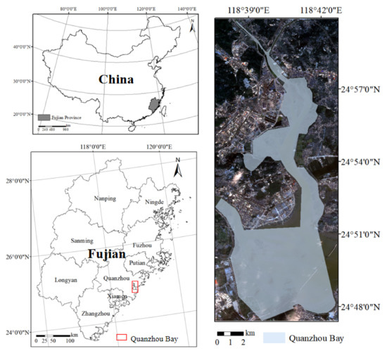
Figure 1.
Location of Quanzhou Bay.
Aquatic animals leave the protected areas due to their natural migration behavior and human factors, such as the presence of cross-sea bridges and conduct of marine economic operations. Therefore, protecting the rare aquatic animals in existing protected areas is critical. In this study, the ecological function area of Puganqiangcheng estuary, in which the Jinjiang River and Luoyang River converge into the sea, as the primary research area to develop a better protection plan and to improve the protective effect for rare aquatic animals.
The government of Quanzhou city has increased the ecological restoration of the QBEWPNR, but the survival of rare marine animals has still been affected by human activities. Thus, the original functional area lacks sufficient protection [34]. Figure 2 presents the Puguncheng estuary wetland ecological function area, which is an essential functional zone of the QBEWNR. The figure reveals that only a few rare aquatic animals appeared in the core or buffer areas; most of their activities are outside the functional zone. The results indicated that the existing ecological function zone of Pugangcheng does not include the primary living habitats of rare aquatic animals and does not sufficiently protect these rare aquatic animals.
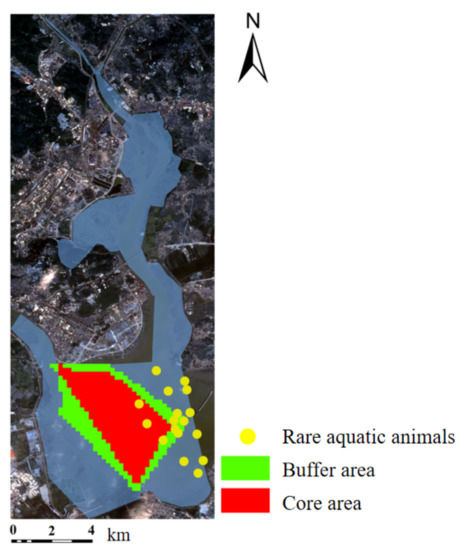
Figure 2.
Distribution of rare aquatic animals and the original reserve.
2.2. Data
We took satellite images with a resolution of 8 m × 8 m captured by the Ziyuan-3 (ZY-3) satellite in 2016 as input and performed preprocessing, including geometric registration, atmospheric correction, and crop. Moreover, we selected the factors of the natural environment and human activity affecting the distribution of rare aquatic animals, including elevation, land use type, and nearest distance to the reserve. Land use types were divided into eight types: forest, mangrove, dry field, paddy field, building, bare land, road, and water using supervised classification and visual interpretation. The nearest distance to infrastructure that significantly affects the activities of rare aquatic organisms, namely paddy fields, roads, and buildings, was determined using the multiring buffer analysis function of ArcGIS 10.2. Grid sections were used as the base unit, and Quanzhou Bay was divided into 200 m × 200 m square grids using ArcGIS 10.2; a total of 5969 grid sections were produced.
The data of rare aquatic animals were derived from a field scientific investigations performed in 2016–2017 (Figure 3). These data were collected by irregular fishing and observation at historical animal occurrence points provided by the Quanzhou Marine Bureau, the nature reserve, and local fishers. The distribution data described the occurrence of rare aquatic animals, such as the time and place of the observation, the species, and the number of animals observed. After data screening and elimination, we obtained 17 rare aquatic animal distribution sites. We assumed that if rare aquatic animals were successfully protected, other aquatic animals would also be protected because rare aquatic animals have strict habitat requirements. Therefore, we only analyzed rare aquatic animals in this study.
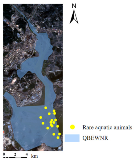
Figure 3.
Distribution of rare aquatic animals.
We randomly selected 75% of the distribution sites as the training set and 25% as the testing set based on the distribution data of the rare aquatic animals. Moreover, we analyzed the relationship between rare aquatic animals and environmental factors using the Maxent model and then predict the potential distribution probability of the rare aquatic animals; this number was used as the ecological suitability value (Figure 4). The included environmental factors were land use type, a digital elevation model, and the nearest distance. The test area under the receiver operating characteristic curve (AUC) value generated from the Maxent model was 0.856, indicating that the model has high prediction accuracy. The potential distribution probability, as shown in Figure 4, was used as the ecological suitability value in the first period.
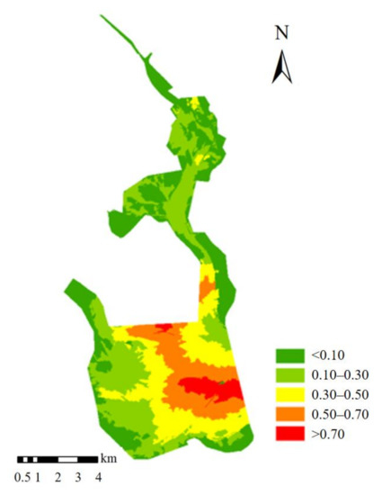
Figure 4.
Potential distribution probability of rare aquatic animals.
3. Methods
An MDP algorithm for nature reserves based on cellular automata (CA), network flow, and other fundamental theories is proposed and developed to address the weaknesses of existing algorithms.
3.1. CA
In protected areas, the ecological benefits of a grid are affected by the surrounding grids. That is, the ecology of the central grid is also optimized if the surrounding grids have good ecology. Moreover, the execution of this process is similar to the theory of the CA model in which each cell is modified based on the state of neighboring cells according to certain system-level rules in the cellular space with discrete units and finite states. Therefore, if the ecological suitability values of adjacent grids are all higher than that of the central grid, the ecological suitability values of the plot is assumed to correspondingly increase. This dynamic updating system for the CA is designed based on this assumption and is expressed as follows:
Here, S is the ecological suitability value of the grids, as presented in Figure 4, is the ecological suitability value of grid i in the period t (such that is the ecological suitability value of grid i in period 1), and is the ecological suitability value between grid i and its adjacent grid j. If the ecological suitability value grid i is less than the adjacent grid j, ; otherwise, . k is a random number that increases the ecological suitability value. The ecological suitability values in the rest periods are produced using the CA dynamic update mechanism in Equation (2). Specifically, the ecological suitability value is the potential distribution probability assigned to each grid, as shown in Figure 4. We then analyze the relationship between grid i and its neighborhood using Equation (2) to adjust the ecological suitability value of grid i and to generate the updated ecological suitability value, , in period 2. These steps are repeated until the final period t to obtain .
3.2. Optimized Objective Function
The objective function of the MPD algorithm has three goals: (1) the maximization of the protection benefits, (2) the minimization of the total perimeter, and (3) the minimization of the number of buffer zones. Finally, the overall protection level was maximized using the multiperiod procedure. The relevant equations are as follows:
We consider the maximization of the ecological value as the objective function of protection benefits in the designed multiperiod programming; this maximization is expressed as follows:
Here, E is the total ecological suitability value of the nature reserve. indicates whether grid i is selected as a core area in period t and is 1 if selected and 0 otherwise. T is the total number of periods. I is the total number of grids.
Moreover, the minimization of the perimeter of the selected grids of core and buffer areas is an additional goal of the objective function. The objective function for minimizing the perimeter of the selected core grids is as follows:
Here, M is the total perimeter of the nature reserve, and is a binary variable indicating whether grid i is selected as part of the core area; it is 1 if selected and 0 otherwise. indicates whether grid i and its adjacent grid j are selected as core areas and form a connection; if so, ; otherwise, .
Furthermore, we minimize the number of grids selected as buffer areas to limit the total number of selected grids; the minimization function is as follows:
Here, N is the total number of buffer grids, and is a binary variable. If grid i is selected as a buffer area, ; otherwise, . We only consider the minimization of the perimeter of the selected core and buffer areas (grids) in the final period because we must first ensure the overall spatial compactness of the core areas, and the buffer areas must surround the core areas.
Finally, we integrate these subobjectives into an objective maximization function formulated as follows:
3.3. Basic Constraints
Two basic constraints were included: cost and type constraints.
3.3.1. Cost Constraints
Grid selection: Each grid can only be selected as a core area once per period as follows:
Grid Aggregation: The construction cost of nature reserves was used to limit the number of grids selected in each period; this limitation is expressed as follows:
Here, is the total number of grids selected in each period.
Minimum Protection of Core Area: The total ecological suitability value of grids selected as core areas in each period must be higher than the minimum protection requirement. The minimum protection requirements are expressed as follows:
Here, is the conservation proportion of the target species in the core area.
3.3.2. Type Constraints
Statistics of Core Area: The number of times a grid i was selected as a core area over all periods dynamically can be formulated as follows:
Here, is a binary variable of 0 or 1, as defined in Equation (4).
Continuity of the Core Area: Core areas should be selected to achieve both spatial continuity and compactness to provide stable breeding sites for species. If grid i and its adjacent grid j are both selected as core areas, they must have a spatial connection. However, if one of these grids is not a core area, this connection may not exist. Core area continuity is expressed as follows:
Partition Attribute: The grid i cannot be selected for both the core and the buffer areas simultaneously.
Here, C and B are binary variables indicating inclusion in the core and buffer areas, respectively.
Partition Connection: A key requirement in nature reserve programming is ensuring that the buffer area surrounds the core area. If grid i is selected as a core area, its adjacent grid j must either be a core area or buffer area. This condition is formulated as follows:
Here, C and B are binary variables indicating inclusion in the core and buffer areas, respectively.
3.4. Multiperiod Constraints Based on Virtual Point
The selected grids must be continuous in all periods to achieve overall spatial continuity of the nature reserve MDP. Figure 5 presents an example of grid selection over three periods indicated by red, green, and blue. Each grid square in Figure 5 is labeled at the upper left corner, and its ecological suitability value is centered. In this example, three grids in each period are selected: blue in period 1, green in period 2, and red in period 3. Although the selected grids in each period are continuous both within and between periods (i.e., local and global continuity, respectively), grid 8 (light grey, ecological suitability value of 0.90) is not included to ensure continuity. This example reveals that the balance between spatial continuity and ecological suitability is critical when selecting grids in reserve programming.
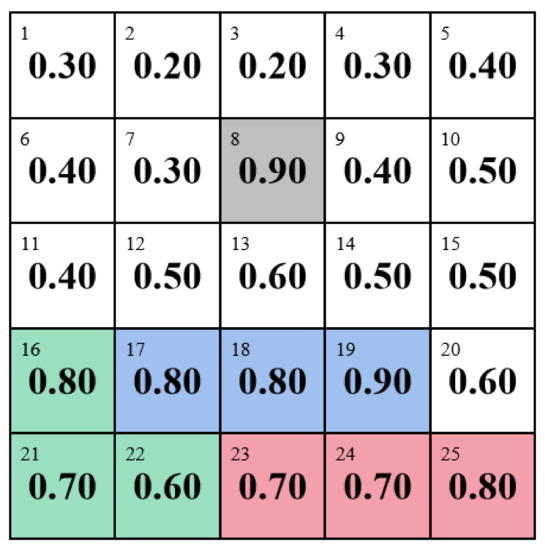
Figure 5.
Example of grid selection with MDP.
Therefore, we introduce the concept of the virtual point in the MDP to balance the conflict between spatial continuity and ecological suitability value when selecting grids. A virtual point is a virtual grid independent of the grids but connected to each grid already selected in the nature reserve, as indicated by the orange square in Figure 6. Grids in each period are selected beginning at the virtual point; this enables selecting grids that are locally discontinuous but globally continuous. For example, the grids selected in periods 2 (green) and 3 (red) are not locally continuous, but the final selection is globally continuous, and the total ecological suitability value is 7—0.20 greater than the result of Figure 5. Thus, the protection benefits can be maximized by setting virtual points to ensure global continuity in each period. We set the relevant constraints of the virtual points as follows:
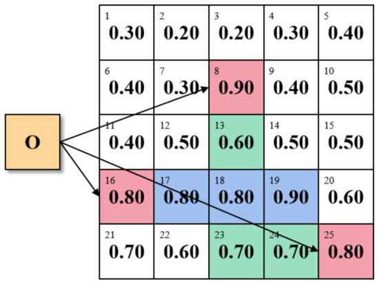
Figure 6.
Example of grid selection using MDP with a virtual point.
Number of Starting Points: The Netflow algorithm specifies the number of starting points to limit the final selection of set regions; the constraint is formulated as follows:
Here, is the flow from the virtual point to grid i in period t. indicates that only one grid is connected to the virtual point in period one to limit the number of reserve areas to 1.
Limitation of Flow Traffic: If grid i is not selected in period t, the inflow number of grid i is 0; otherwise, the maximum number of the inflow from the adjacent grid j to grid i is (M − 1). The constraint formula is expressed as follows:
Here, is the total number of flows from core grid j to its adjacent core grid i in period t. is a binary variable; indicates that grids i and j are connected; otherwise, . is the set of grid numbers adjacent to grid i. M is a constant and can be set to an arbitrary value but should be larger than the total number of grids.
Quantity Relationship between Inflow and Outflow: The difference between the outflow and inflow of grid i in period t must be greater than or equal to . Its constraint is formulated as follows:
Here, is the total number of flows from core grid i to an adjacent core grid j in period t. If grid i in period t is not connected to the virtual point, its outflow is greater than or equal to the inflow + 1.
Continuity constraint between the virtual point and the core grid: If grid i in period t is connected to the virtual point, it must be selected as a core grid. The formulation is expressed as follows:
Multiperiod grid continuity: If grid i connects to the virtual point, it must connect to grid j, selected as a core grid in the previous period, to ensure the grid’s continuity between each period. We express the constraint as the following formulation:
Here, indicates whether grid j adjacent to grid i is selected as a core area in period . If grid j is selected in period t − 1, ; otherwise, .
4. Results
4.1. Parameter Settings
We programmed the MDP model with the branch and bound algorithm of the Gurobi Optimizer. The parameters were adjusted several times; the optimal set is as follows: , , and a total of 300 core grids. Thus, we selected 100 core grids () in each of the three periods (). Moreover, grids with high ecological suitability values improve the values of surrounding grids due to regionalism. Therefore, we set k to be in CA.
4.2. Ecological Suitability Value
The frequency distribution for ecological suitability values over various periods with the adjustment of CA is presented in Figure 7. Rectangular bars with a greater width indicate higher frequencies of the ecologically suitable value. The number of grids with low ecological suitability values decreased gradually because of the positive influence of the reserve construction and the surrounding grids with a high ecological suitability value. The number of grids with a high ecological suitability value also increased, but this change was small. Thus, the overall ecological environment of Quanzhou Bay improved.
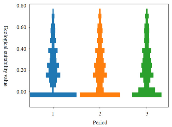
Figure 7.
Frequency distribution of multiperiod ecological suitability values.
A visualization of the ecological suitability values in various periods is displayed in Figure 8. The overall distribution of ecological suitability values in Quanzhou Bay did not change significantly beacuse k was set to 0.05. However, this agreed with typical natural processes, which have only small variations in short periods. The red grids with high ecological suitability values () in the north and east gradually expanded outward, and dark green grids with the lowest ecological suitability value () transformed into light green grids with low ecological suitability values (). Overall, some grids in each color category were transformed into the grids of a higher color category, as depicted in Figure 7.
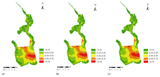
Figure 8.
Visualization of multiperiod ecological suitability values: (a) Period 1; (b) Period 2; (c) Period 3.
4.3. Multiperiod Dynamic Changes
The results of the MDP algorithm for nature reserve planning is presented in Table 1 and Figure 9. The difference between total ecological suitability values in the three periods was small because 100 grids were selected in each period. The total ecological suitability value of the first period was the largest because grids with the largest ecological values were selected first in the MDP algorithm. The total ecological suitability value of period 3 was greater than that of period 2 because period 2 is an intermediate transitional period; grids with the largest ecological values were not selected in period 2 to ensure continuity. A total of 300 grids were selected for the core area, and the total ecological suitability value was 185.51 with a mean ecological suitability value of 0.62. These results reveal that the programming is effective for environmental protection.

Table 1.
Comparison results of the selected core areas using the MDP algorithm in three periods.
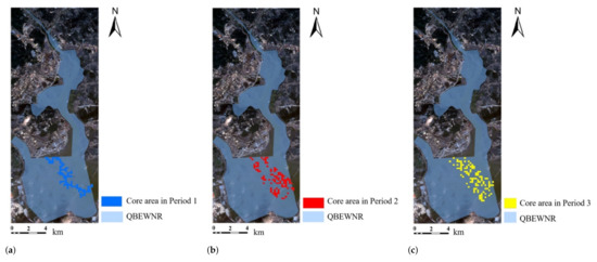
Figure 9.
Selected core areas in each period: (a) Period 1; (b) Period 2; (c) Period 3.
Moreover, we present the visualization results of multiperiod programming for the selected core areas in each period in Figure 9. The blue, red, and yellow areas indicate the core grids selected in periods 1 to 3; the distribution of the selected grids significantly differ between periods. The selected grids in period 1 are continuous from northwest to southeast; this distribution was consistent with the distribution of grids with high ecological suitability values (), as shown in Figure 8a. The selected grids in periods 2 and 3 were distributed discretely from northwest to southeast and gradually spread outward around the core area secreted in period 1. This distribution was consistent with the distribution of below-average ecological suitability values (), as presented in Figure 8b,c. The programming results for the two periods were discrete, but the final core area had spatial continuity and compactness, as presented in Figure 10.
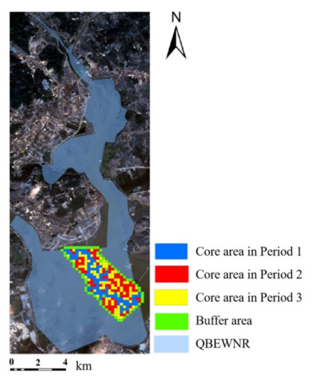
Figure 10.
Integration of the selected core grids.
Figure 10 presents the final core area and buffer areas (grids) selected by the MDP algorithm; green grids indicate the buffer areas. The selected buffer grids surround the core area and fill holes to increase the compactness of the protected area. Furthermore, we present a comparison of the original nature reserve and that of the MDP algorithm in Table 2. The original reserve had 339 core grids and 209 buffer grids; the MDP algorithm selected 300 grids and 72 grids. Thus, the reserve selected by the MDP algorithm had fewer core and fewer buffer grids.
Table 2.
Statistics of the MDP algorithm and original reserves.
Table 2 reveals that the MDP algorithm also outperformed the original reserve in most measures of ecological suitability. Despite selecting fewer grids, the MDP reserve had far higher total and mean ecological suitability values than the original reserve. The original reserve only had a superior result for the total ecological suitability value of the buffer zone compared with the MDP reserve (47.05 vs. 27.41, respectively); however, this result can be attributed to the inefficient buffer zone selection in the original reserve, as revealed by the mean values (0.23 vs. 0.38, respectively). Therefore, the MDP algorithm reserve represents a substantial improvement compared to the existing reserve both for total protection and efficiency.
5. Discussion
5.1. Multiperiod Programming
The proposed MDP algorithm was used for nature reserve design based on IP, including the innovation of multiperiod programming. The Chinese government typically implements designs for natural areas in decadal plans. They first designate a large area as a nature reserve and gradually develop each area according to project requirements and funding. Most studies [22,24,27,31] on nature reserves have schemes that design the core, buffer, and experimental zones of the reserve in a single step. They focus on selecting core or buffer zones, improving the protection effect, and realizing spatiality.
Moreover, Jafari et al. [30] first proposed multiperiod programming in a nature reserve by considering the connectivity between different periods. However, the core and buffer areas were not divided, and the reserve was not compact; these are key requirements for nature reserve design. Therefore, we propose the novel MDP algorithm to gradually expand the reserve around the sites selected in the first period until an overall optimal solution is determined. The MDP algorithm satisfies the requirements for long-term construction of nature reserves.
5.2. Ecological Dynamic Variation
The principle used in CA that areas with good ecological environments improve their surroundings [35,36] was used to compare nearby sites to increase the actual protection effect through the adjustment of ecological values in each period. The variation of ecological suitability values in numerical frequency and spatial distribution is small, but natural changes of ecological environments in a short period are typically small [36]; thus, CA can simulate ecological improvements in the nature reserve. Overall, the overall protection benefit is significantly improved because priority sites were targeted. CA was used to quantify dynamic changes in ecological value, consistent with the idea that the environmental state changes as the reserve is constructed [31].
5.3. Continuity through Virtual Points
One of the main contributions of this study is to realize continuity with virtual points. Existing algorithms [23,24,32,33] can achieve continuity for a single period or multiple periods but inevitably select grids with low ecological value to ensure continuity, reducing the average ecological benefit. Virtual points were used in reserve planning to ensure that ecological benefits were maximized and to achieve continuity for each period and the whole, despite discontinuity within a single period.
Moreover, landscape fragmentation is a key cause of biodiversity loss. Thus, spatial continuity is a key factor in reserve construction. MDP for a nature reserve can be regarded as dynamic path planning. Sites with low ecological value are considered obstacles, and the selected sites are those with high environmental protection in path planning [37]. Finally, an optimal path with no collisions and the shortest distance is planned.
5.4. Number of Zones
Most studies have used three divisions [38] in nature reserve programming, but some studies have used two zones. This transformation from three zones to two zones facilitates the management of the reserves; it is not conducted because three zones are unscientific or unreasonable [3]. In theoretical calculations, the reserve should be programmed with three zones, including the core area, buffer area, and experimental area, to arrange the results into two zones according to the protection requirements.
5.5. Limitations and Outlook
The MDP algorithm could be further optimized with stochastic optimization algorithms produced by simulating the behavior of natural biological groups, such as the particle swarm optimization algorithm or the ant colony algorithm. Moreover, CA was used to generate the adjusted ecological suitability values based on the original ecological suitability value of the sites instead of based on the results of grid selection in each period. Adjustment based on grid selections could have superior performance. Moreover, future studies could investigate the characteristics of estuarine wetlands in Quanzhou Bay, including rare aquatic animals, the ecological suitability value of essential wetland plants, and an evaluation system of ecological suitability. For example, the distribution of essential wetland plants, such as mangroves, could be used to calculate the ecological suitability value. An ecological suitability evaluation system for estuarine wetlands would be based on a comprehensive evaluation of aspects, such as primary species distribution, wetland characteristic species distribution, and economic development impact.
Furthermore, the IP was investigated based on 200 m × 200 m grids due to computer memory limitations. In the future, we could use grids with smaller sizes for more precise planning or irregular small class planning. Furthermore, we will explore the influence of the Gurobi parameter setting and the network model constraints on the computational cost.
6. Conclusions
The distribution of rare aquatic animals simulated by Maxent was used to determine ecological suitability values in the QBEWNR. We used CA to simulate variations in ecological suitability values during different periods of partitioning the QBEWNR. Finally, we proposed a novel MDP algorithm based on network flow theory to design the nature reserve. The MDP algorithm satisfies the primary optimization constraints, such as cost, partitioning, and continuity.
Moreover, we introduced virtual points in the MDP algorithm to design multiperiod constraints, such as numerous starting points, networked traffic, and continuity between virtual points and core sites. The MDP algorithm maximized the ecological suitability value, minimized the perimeter, and minimized the number of sites for the reserve and thus rationally selected a protection scheme for the QBEWNR over an extended period.
The results reveal that the total ecological suitability value (212.92) of the reserve generated by the MDP algorithm was substantially higher than that of the original reserve (111.35). Moreover, the number of selected sites (372) selected by MDP was substantially lower than the original reserve (547), demonstrating the superior performance of the MDP algorithm.
Author Contributions
Conceptualization, C.-W.L.; methodology, C.-W.L. and W.T.; validation, C.-W.L. and W.T.; investigation, C.-W.L. and W.T.; writing—original draft preparation, C.-W.L., W.T. and Y.H.; writing—review and editing, C.-W.L. and J.L. All authors have read and agreed to the published version of the manuscript.
Funding
This work was supported in part by the China Postdoctoral Science Foundation under Grant 2018M632565, in part by the Channel Post-Doctoral Exchange Funding Scheme, in part by the Natural Science Foundation of Fujian Province under Grant 2021J01128, and in part by the Youth Program of Humanities and Social Sciences Foundation, Ministry of Education of China, under Grant 18YJCZH093.
Institutional Review Board Statement
Not applicable.
Informed Consent Statement
Not applicable.
Data Availability Statement
Data sharing not applicable.
Conflicts of Interest
The authors declare no conflict of interest.
Abbreviations
The following abbreviations are used in this manuscript:
| MDP | Multiperiod Dynamic Programming |
| NR | Nature Reserve |
| SCP | Set Covering Problem |
| MCP | Maximal Covering Probem |
| IP | Integer Programming |
| CA | Cellular Automata |
| SCP | Set Covering Problem |
| TLP | Tail Length Problem |
| NFP | Network Flow Problem |
| SA | Simulated Annealing |
References
- Liu, P.; Jiang, S.; Zhao, L.; Li, Y.; Zhang, P.; Zhang, L. What are the benefits of strictly protected nature reserves? Rapid assessment of ecosystem service values in Wanglang Nature Reserve, China. Ecosyst. Serv. 2017, 26, 70–78. [Google Scholar] [CrossRef]
- The State Council. Regulations on the Management of Nature Reserves in People’s Republic of China; The State Council: Beijing, China, 1994.
- Tang, J.; Lu, H.; Xue, Y.; Li, J.; Li, G.; Mao, Y.; Deng, C.; Li, D. Data-driven planning adjustments of the functional zoning of Houhe National Nature Reserve. Glob. Ecol. Conserv. 2021, 29, e01708. [Google Scholar] [CrossRef]
- Aspinall, R.J. Use of logistic regression for validation of maps of the spatial distribution of vegetation species derived from high spatial resolution hyperspectral remotely sensed data. Ecol. Model. 2002, 157, 301–312. [Google Scholar] [CrossRef]
- Holder, A.M.; Markarian, A.; Doyle, J.M.; Olson, J.R. Predicting geographic distributions of fishes in remote stream networks using maximum entropy modeling and landscape characterizations. Ecol. Model. 2020, 433, 109231. [Google Scholar] [CrossRef]
- Phillips, S.J.; Anderson, R.P.; Schapire, R.E. Maximum entropy modeling of species geographic distributions. Ecol. Model. 2006, 190, 231–259. [Google Scholar] [CrossRef] [Green Version]
- Renner, I.W.; Warton, D.I. Equivalence of MAXENT and Poisson point process models for species distribution modeling in ecology. Biometrics 2013, 69, 274–281. [Google Scholar] [CrossRef]
- Kingsland, S.E. Creating a science of nature reserve design: Perspectives from history. Environ. Model. Assess. 2002, 7, 61–69. [Google Scholar] [CrossRef]
- Ricklefs, R.E. A comprehensive framework for global patterns in biodiversity. Ecol. Lett. 2004, 7, 1–15. [Google Scholar] [CrossRef] [Green Version]
- Domíguez-Vega, H.; Monroy-Vilchis, O.; Balderas-Valdivia, C.J.; Gienger, C.; Ariano-Sánchez, D. Predicting the potential distribution of the beaded lizard and identification of priority areas for conservation. J. Nat. Conserv. 2012, 20, 247–253. [Google Scholar] [CrossRef]
- Gastón, A.; Garcia-Vinas, J.I. Modelling species distributions with penalised logistic regressions: A comparison with maximum entropy models. Ecol. Model. 2011, 222, 2037–2041. [Google Scholar] [CrossRef]
- Vaz, S.; Martin, C.S.; Eastwood, P.D.; Ernande, B.; Carpentier, A.; Meaden, G.J.; Coppin, F. Modelling species distributions using regression quantiles. J. Appl. Ecol. 2008, 45, 204–217. [Google Scholar] [CrossRef] [Green Version]
- Pineda, E.; Lobo, J.M. Assessing the accuracy of species distribution models to predict amphibian species richness patterns. J. Anim. Ecol. 2009, 78, 182–190. [Google Scholar] [CrossRef] [PubMed]
- Yu, H.; Cooper, A.R.; Infante, D.M. Improving species distribution model predictive accuracy using species abundance: Application with boosted regression trees. Ecol. Model. 2020, 432, 109202. [Google Scholar] [CrossRef]
- Ingram, M.; Vukcevic, D.; Golding, N. Multi-output Gaussian processes for species distribution modelling. Methods Ecol. Evol. 2020, 11, 1587–1598. [Google Scholar] [CrossRef]
- Beasley, J.E.; Chu, P.C. A genetic algorithm for the set covering problem. Eur. J. Oper. Res. 1996, 94, 392–404. [Google Scholar] [CrossRef]
- Kinney, G.W.; Barnes, J.W.; Colletti, B.W. A reactive tabu search algorithm with variable clustering for the unicost set covering problem. Int. J. Oper. Res. 2007, 2, 156–172. [Google Scholar] [CrossRef]
- Possingham, H.; Ball, I.; Andelman, S. Mathematical methods for identifying representative reserve networks. In Quantitative Methods for Conservation Biology; Springer: Berlin/Heidelberg, Germany, 2000; pp. 291–306. [Google Scholar] [CrossRef] [Green Version]
- Chern, C.C.; Hsieh, J.S. A heuristic algorithm for master planning that satisfies multiple objectives. Comput. Oper. Res. 2007, 34, 3491–3513. [Google Scholar] [CrossRef]
- Underhill, L. Optimal and suboptimal reserve selection algorithms. Biol. Conserv. 1994, 70, 85–87. [Google Scholar] [CrossRef]
- Ando, A.; Camm, J.; Polasky, S.; Solow, A. Species distributions, land values, and efficient conservation. Science 1998, 279, 2126–2128. [Google Scholar] [CrossRef]
- Camm, J.D.; Norman, S.K.; Polasky, S.; Solow, A.R. Nature reserve site selection to maximize expected species covered. Oper. Res. 2002, 50, 946–955. [Google Scholar] [CrossRef]
- Önal, H.; Briers, R.A. Optimal selection of a connected reserve network. Oper. Res. 2006, 54, 379–388. [Google Scholar] [CrossRef] [Green Version]
- Önal, H.; Wang, Y. A graph theory approach for designing conservation reserve networks with minimal fragmentation. Netw. Int. J. 2008, 51, 142–152. [Google Scholar] [CrossRef]
- Williams, J.C. A zero-one programming model for contiguous land acquisition. Geogr. Anal. 2002, 34, 330–349. [Google Scholar] [CrossRef]
- Williams, J.C. Optimal reserve site selection with distance requirements. Comput. Oper. Res. 2008, 35, 488–498. [Google Scholar] [CrossRef]
- Jafari, N.; Hearne, J. A new method to solve the fully connected reserve network design problem. Eur. J. Oper. Res. 2013, 231, 202–209. [Google Scholar] [CrossRef]
- Costello, C.; Polasky, S. Dynamic reserve site selection. Resour. Energy Econ. 2004, 26, 157–174. [Google Scholar] [CrossRef] [Green Version]
- Tóth, S.F.; Haight, R.G.; Rogers, L.W. Dynamic reserve selection: Optimal land retention with land-price feedbacks. Oper. Res. 2011, 59, 1059–1078. [Google Scholar] [CrossRef] [Green Version]
- Jafari, N.; Nuse, B.L.; Moore, C.T.; Dilkina, B.; Hepinstall-Cymerman, J. Achieving full connectivity of sites in the multiperiod reserve network design problem. Comput. Oper. Res. 2017, 81, 119–127. [Google Scholar] [CrossRef]
- Álvarez-Miranda, E.; Goycoolea, M.; Ljubić, I.; Sinnl, M. The generalized reserve set covering problem with connectivity and buffer requirements. Eur. J. Oper. Res. 2021, 289, 1013–1029. [Google Scholar] [CrossRef] [Green Version]
- Lin, C.W.; Liu, J.; Huang, J.; Zhang, H.; Lan, S.; Hong, W.; Li, W. Space-ecology set covering problem for modeling Daiyun Mountain Reserve, China. In IOP Conference Series: Earth and Environmental Science; IOP Publishing: Bristol, UK, 2018; Volume 121, p. 032040. [Google Scholar] [CrossRef]
- Lin, C.W.; Tu, W.H.; Liu, J.F. Dual-Flow Structure to Design a Continuous and Compact Nature Reserve. IEEE Access 2019, 7, 35220–35230. [Google Scholar] [CrossRef]
- Yang, Y.; Ding, J.; Chi, Y.; Yuan, J. Characterization of bacterial communities associated with the exotic and heavy metal tolerant wetland plant Spartina alterniflora. Sci. Rep. 2020, 10, 17985. [Google Scholar] [CrossRef] [PubMed]
- Tyrväinen, L.; Ojala, A.; Korpela, K.; Lanki, T.; Tsunetsugu, Y.; Kagawa, T. The influence of urban green environments on stress relief measures: A field experiment. J. Environ. Psychol. 2014, 38, 1–9. [Google Scholar] [CrossRef]
- Wolf, K.L.; Measells, M.K.; Grado, S.C.; Robbins, A.S. Economic values of metro nature health benefits: A life course approach. Urban For. Urban Green. 2015, 14, 694–701. [Google Scholar] [CrossRef]
- Wang, N.; Xu, H. Dynamics-constrained global-local hybrid path planning of an autonomous surface vehicle. IEEE Trans. Veh. Technol. 2020, 69, 6928–6942. [Google Scholar] [CrossRef]
- Wang, C.; Wang, W.; He, S.; Du, J.; Sun, Z. Sources and distribution of aliphatic and polycyclic aromatic hydrocarbons in Yellow River Delta Nature Reserve, China. Appl. Geochem. 2011, 26, 1330–1336. [Google Scholar] [CrossRef]
Publisher’s Note: MDPI stays neutral with regard to jurisdictional claims in published maps and institutional affiliations. |
© 2022 by the authors. Licensee MDPI, Basel, Switzerland. This article is an open access article distributed under the terms and conditions of the Creative Commons Attribution (CC BY) license (https://creativecommons.org/licenses/by/4.0/).