Article

Intense Pasture Management in Brazil in an Integrated Crop-Livestock System Simulated by the DayCent Model

by
Yane Freitas Silva
1,*,
Rafael Vasconcelos Valadares
2,
Henrique Boriolo Dias
2,
Santiago Vianna Cuadra
3,
Eleanor E. Campbell
4,
Rubens A. C. Lamparelli
2,
Edemar Moro
5,
Rafael Battisti
6,
Marcelo R. Alves
5,
Paulo S. G. Magalhães
2 and
Gleyce K. D. A. Figueiredo
1
1
School of Agricultural Engineering (FEAGRI), University of Campinas (UNICAMP), Campinas 13083-875, SP, Brazil
2
Centre of Energy Planning (NIPE), University of Campinas (UNICAMP), Campinas 13083-875, SP, Brazil
3
Embrapa Agricultural Informatics (CNPTIA), Brazilian Agricultural Research Company (EMBRAPA), Campinas 13083-886, SP, Brazil
4
Earth Systems Research Center, University of New Hampshire, Durham, NH 03824, USA
5
Department of Agronomy, University of Western São Paulo, Presidente Prudente 19067-175, SP, Brazil
6
Agronomy School, Federal University of Goiás, Goiânia 74690-900, GO, Brazil
*
Author to whom correspondence should be addressed.
Sustainability 2022, 14(6), 3517; https://doi.org/10.3390/su14063517
Submission received: 22 February 2022 / Revised: 4 March 2022 / Accepted: 10 March 2022 / Published: 17 March 2022

Abstract

:
Process-based models (PBM) are important tools for understanding the benefits of Integrated Crop-Livestock Systems (ICLS), such as increasing land productivity and improving environmental conditions. PBM can provide insights into the contribution of agricultural production to climate change and help identify potential greenhouse gas (GHG) mitigation and carbon sequestration options. Rehabilitation of degraded lands is a key strategy for achieving food security goals and can reduce the need for new agricultural land. This study focused on the calibration and validation of the DayCent PBM for a typical ICLS adopted in Brazil from 2018 to 2020. We also present the DayCent parametrization for two forage species (ruzigrass and millet) grown simultaneously, bringing some innovation in the modeling challenges. We used aboveground biomass to calibrate the model, randomly selecting data from 70% of the paddocks in the study area. The calibration obtained a coefficient of determination (R2) of 0.69 and a relative RMSE of 37.0%. During the validation, we used other variables (CO2 flux, grain biomass, and soil water content) measured in the ICLS and performed a double validation for plant growth to evaluate the robustness of the model in terms of generalization. R2 validations ranged from 0.61 to 0.73, and relative RMSE from 11.3 to 48.3%. Despite the complexity and diversity of ICLS results show that DayCent can be used to model ICLS, which is an important step for future regional analyses and large-scale evaluations of the impacts of ICLS.

1. Introduction

Integrated Crop-Livestock Systems (ICLS) are defined by the diversification, rotation, consortium, and succession of agriculture and livestock inside the same area, allowing benefits between these two activities and the economic use of soil over the year [1]. The adoption of ICLS comprises 10–15 million ha (5% of total) of the area under agriculture and livestock in Brazil [2], which represents a significant opportunity to improve the sustainability of agricultural systems [3], especially in degraded areas and over sandy soils.
With the integration of soybean and mixed-pasture, ICLS impacts plant growth as the nitrogen (N) supplied by legumes (for instance, soybean) is absorbed more efficiently than that applied through mineral fertilization, stimulating plant growth and biomass quality, or both, through increased N uptake [4]. Lower dry matter production in grass monoculture pastures tends to decrease soil moisture, organic carbon (C), and total N compared to ICLS [5].
In this context, the applications of process-based ecosystem models are fundamental to evaluate and improve the level of understanding of these systems and predict processes such as plant growth, C dynamics, and carbon dioxide (CO2) flux. The advantages of using process-based ecosystem models are the possibility of extrapolation of the simulations from an experimental site to different sites and climate conditions [6], making it possible to have a consistent evaluation of other production systems [7,8,9,10].
DayCent is an ecosystem process-based model, and when properly validated by field observations is a powerful tool to investigate the effects of management practices on greenhouse gases (GHG) emissions or soil organic carbon (SOC) changes in different ecosystems, soil types, and climates [11]. Frolking et al. [12] demonstrated the ability of the DayCent model [13,14] to simulate soil water content, mineral N levels, nitrous oxide (N2O), and CO2 emissions for various systems, including a native shortgrass steppe in Colorado, a ryegrass pasture in Scotland, and perennially cropped soils in Germany.
In tropical and subtropical agriculture, simulations aiming to test the performance of DayCent in predicting SOC, biomass production, crop yield, and N2O fluxes were also performed [15]. They evaluated the model for agroecosystems under succession/rotational managements with crops such as wheat, soybean, sorghum, oat, and maize considering different management and climate scenarios in southern Brazil, and the predictive accuracy varied from poor (plant growth) to adequate (SOC and N2O fluxes) [15]. Damian et al. [16] evaluated the effects of converting poorly managed pastures to more intensive and diversified pasture management systems in Brazil, such as ICLS, on long-term soil C stocks and microbial biomass C increased with the conversion of pastures to ICLS using the DayCent model.
However, due to the diversity and complexity of ICLS, model predictions need to be adjusted and validated considering the region and system adopted. For instance, complex agroecosystem designs such as ICLS generally present the different combinations of plant species, directly impacting the soil C fluxes [17]. Additionally, after implementation, ICLS often have higher stocking rates and differences in animal trampling and excretion patterns [18] and the additional inputs with fertilization and biological N fixation [17,19]. Furthermore, the CO2 assimilated by the photosynthetic process is the basis of crop production [20]. Therefore, it is necessary to consider that the ICLS is the system that fixes the most CO2, and emits the least GHG, throughout the year. This information is essential for the current global scenario, mainly due to carbon trading, an environmental management tool for controlling carbon emissions [21].
In this study, we focus on evaluating the DayCent performance in simulating plant growth, soil moisture, and CO2 fluxes as this kind of system presents different patterns of inputs, outputs, and, very likely, of model coefficients and rates related to the different processes [13,14,22,23]. To our knowledge, despite the importance of ICLS, there are few studies of the DayCent model in this type of agricultural system in Brazil and worldwide, mainly for sandy soils. This study aids large-scale simulations of ICLS impacts on the environment, mainly due to the importance of C trading, which may boost the use of ICLS according to the requests of the Sustainable Development Goals (SDGs) [24], to increase agroecosystem production (SDG2—Zero Hunger) [25], mitigate climate change (SDG13—Climate Action) [26], and recover degraded pastures (SDG15—Life on Land) [27]. In this context, the objective of this study was to calibrate and validate the DayCent model to estimate an ICLS with a succession of soybean followed by mixed-pasture (ruzigrass and millet) in tropical Brazil. To do that, we also addressed the implementation in DayCent of two pastures grown simultaneously.

2. Materials and Methods
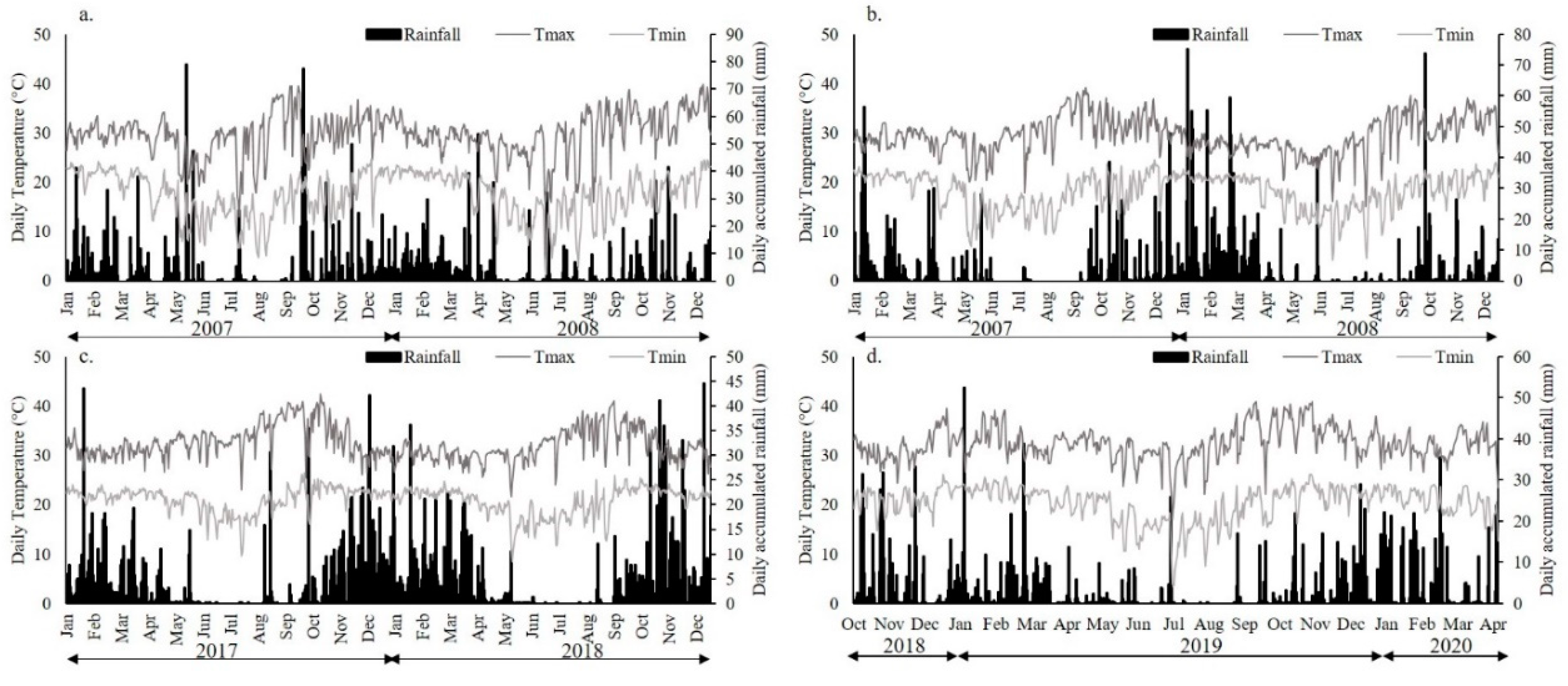
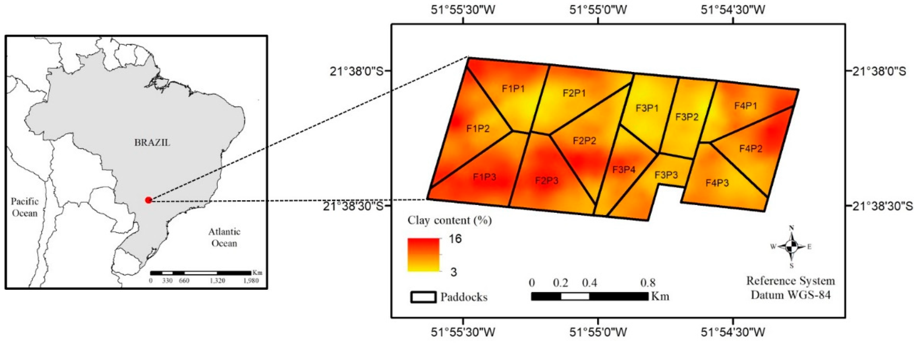
2.1. Field Data

The data were obtained from a commercial area of 200 ha divided into four fields of 50 ha, located at the municipality of Caiuá, in the western region of São Paulo state, Brazil (21°38′ S and 51°54′ W; Figure 1). The climate is classified as tropical with a dry winter season (Aw), according to Köppen’s classification [28]. The accumulated rainfall, mean minimum and maximum daily air temperatures during the monitored period were, respectively, 2021.8 mm, 20.4, and 32.4 °C, from October 2018 to April 2020 (Figure 2). The meteorological data were obtained by prediction of worldwide energy resources (hereafter called NASA/POWER; https://power.larc.nasa.gov/data-access-viewer/, accessed on 2 July 2021), which has shown to be a good source for model simulations under Brazilian conditions [29,30,31].
The soil of the area is formed from rocks of Bauru Group sandstone of the Cretaceous period [32] and has the dominance of kaolinite in the clay fraction [33]. The soil of the region is classified as Oxisol with a sandy loam texture [34]. The slope between 3 to 7% is classified as “gently sloping” according to USDA classification [35]. Elevation range is between 310 m and 370 m above mean sea level.
The pre-experiment started in the area defined by the Atlantic Forest biome (the vegetation is constituted of a dense forest of medium and large trees with a large amount of plant residue on the soil surface), which had extensive pasture without proper management (estimated beginning of extensive pasture in 1984 by farm data), either with fertilizers or conventional management practices, such as recovery/renewal pastures or animal management. In August 2007, 0.5 Mg ha−1 of dolomitic limestone was applied, followed by conventional practices of ploughing and harrowing (Figure 3). Furthermore, 400 and 200 kg ha−1 were applied of reactive rock phosphate (35% P2O5 total and 12.5% P2O5 in citric acid solution) and soluble fertilizer NPK (4-21-15), respectively.
Single forage (Urochloa brizantha cv. Marandu) was sown in October 2007. Fertilization was carried out annually, consisting of the application of 300 kg ha−1 of the NPK formulation 20-10-10, and this fertilization was occasionally applied only to maintain the grazing.
Heifers aged 2 to 3 years (450 kg animal−1) were kept in extensive pasture in the experimental area throughout the period (2007–2018), with an average stocking rate around 1.6 to 1.8 animal unit (AU) ha−1. All these land-use data were used to schedule the pre-experiment for the study area.
This pre-experiment simulation covers 1984 to 2017 with extensive pasture and management, shown in Figure 3. Soil cover reported by the farm was made of crops in previous periods through local information and confirmation via the SATVEG platform [36]. We modified the fertilization, crop, and grazing defaults for the pre-experiment to represent the land-use change and management. At the end of the pre-experiment simulation, total SOC (in the soil layer from 0–0.2 m) simulated was compared with those observed in the field from the initial soil analyses made before implementing the ICLS.
During the ICLS—experiment period from 2018 to 2020, the ICLS consisted of two phases: summer season (soybean) and winter season (mixed-pasture) (Figure 3, Table A1). Preparation for the ICLS began in mid-August 2018, with the application of 1.5 Mg ha−1 of gypsum plus limestone. Then, approximately 5 Mg ha−1 of organic compost was applied to the terrace channel of the area in early September. The herbicide application was carried out to enter the new crop, following common practices in the other farms of the group.
The area was divided into four fields of about 50 ha each (Figure 1), in which soybean was sown under no-tillage. Different varieties were sown in each field (Table A1), with dates ranging from 18 to 22 November 2018, for the first soybean cycle. Monoammonium phosphate (MAP) and potassium chloride (KCl) were applied in 250 and 150 kg ha−1 in the soybean planting furrow under no-tillage. The soybean harvest took place from 30 March to 5 April 2019.
For the implantation of the pasture, the fields were divided into paddocks each to obtain a rotating grazing system, totaling 13 paddocks (Figure 1). Winter season cultivation and pasture intercropping began simultaneously after the soybean harvest (2 to 6 April 2019). The pasture was composed of a consortium of millet (Pennisetum glaucum) and ruzigrass (Urochloa ruziziensis) with a seeding rate in the proportion of 15 kg ha−1 and 5 kg ha−1 of seeds, respectively. The rotational system consisted of two or three grazing events in each paddock depending on each field of pasture development, the first of which was of greater intensity (paddock average ≈ 156 cattle paddock−1), the second of lesser intensity (paddock average ≈ 84 cattle paddock−1), and the third of medium intensity (paddock average ≈ 109 cattle paddock−1), which was not performed for field 4 (Table A1). In November, the herbicide was applied in the total area, and the preparation for planting the second soybean in the area was carried out.
The second soybean cycle started between 11 and 15 December 2019, with the harvest being carried out from 4 to 9 April 2020. The same soybean varieties from the last cultivation were sown, but varied among the fields (Table A1). Like the first soybean cycle, the second was fertilized during the sowing with the previously mentioned fertilizer method.
Soil samples were taken in October 2018 for the chemical and physical characterization of each paddock (Table 1 and Figure 1). Sampling field collections were performed to obtain soil physical and chemical characteristics, aboveground biomass and grain at harvest, and volumetric soil water content (VWC) (Table A2). The initial measurements of the experimental area were performed before the ICLS implementation by stratified systematic unaligned sampling within each paddock and with a variation of 0–1.0 m for soil and surface for plant data at the end of the extensive pasture period (Table 1 and Table A2).
Subsequently, physical (clay, sand, and bulk density) and chemical (total C and pH) analyses were performed following protocols from the Manual of soil analysis methods [38]. The bulk density (volumetric ring method) was determined by differentiating the sampling by depth with three repetitions for 0–0.20 m spaced by 0.05 m depth in each sample, one of 0.25–0.30 m, one sample of 0.35–0.40 m, a 0.65–0.70 m sample, and a 0.95–1.00 m sample. For the total C content, samples were collected at the same points and depth as the bulk density of the soil. These were air-dried, sieved with a 2.0 mm diameter sieve, then manually ground in a mortar and pistil, and a new 0.177 mm sieving [38]. Then, the samples were sent to the laboratory, which performed the analysis by dry oxidation by the elemental analyzer CHNS-O. This method is based on the oxidation of samples at high temperatures (approximately 1000 °C). The samples were placed in a tin capsule, which does not contain C. After total combustion, the gases containing each element were separated and the concentrations measured by different infrared detectors.
Regular collections of the aboveground biomass were performed after the ICLS phase started, varying from two to three repetitions for each paddock. For soybeans, one linear meter was considered, according to the sowing row, and for mixed-pasture, an area of 1 m2, in both cases cutting the biomass close to the ground (≈0.01 m) (Figure 1, Table A2). The aboveground biomass material was dried in an oven with forced air circulation (65–70 °C) until reaching constant mass. Biomass C content was calculated considering the factor of 0.475 [39], with all the results expressed in g C m−2.
Furthermore, VWC was determined by gravimetric water content measurements multiplied by soil density (0–0.05 m depth, drying in forced air circulation oven) using the same sampling scheme in which biomass measurements were taken. CO2 flux was determined using a gas flow quantification chamber (LI 8100A, LI-COR Environmental, Lincoln, NE, USA), with nine samples per paddock on three different dates different from the aboveground biomass collection dates for the mixed-pasture, four for the second soybean, and two for the transition between seasons (Table A2). The measurement was carried out with a duration of 1.5 min for each collection point and carried out around 7 a.m. to avoid soil temperature instability. For the standardization of the CO2 flux values, it was assumed that for the DayCent output, the CO2 flux is constant throughout the day, that is ((CO2) total = 24 (CO2) hours) to compare with that measured and have a simplification of the soil respiration processes.

2.2. SOC Reference Data from the Literature

To start the equilibrium modeling, it was necessary to use literature data on SOC from native vegetation close to the study area in Caiuá, São Paulo (SP). Published data from Rigolin et al. [40], compared the C stocks (0–0.2 m) and the different managements in an area in Presidente Prudente, SP (22°07′ S and 51°27′ W), and used data from native vegetation, without human intervention for 50 years; C stocks were compared with the one simulated by DayCent because it was from the same biome and with similar climatic and soil conditions (Figure A1 detail d). For the extensive pasture, we used data collected on 28 October 2018, which collected soil bulk density and total soil C content up to 1 m depth to estimate C stocks and aboveground biomass for all paddock points in the study area in Caiuá, SP.
To increase confidence that the model is applicable for different areas of ICLS after the calibration, we employed data of the aboveground biomass from the literature called other regions (OR) using [41,42] datasets, both with an ICLS with mixed-pastures and soybean. The same calibrated parameters were used without any change, changing only the input data and the management adopted in the model. Souza’s [41] study was carried out in Rondonópolis, Mato Grosso state (MT), Brazil (16°27′ S and 54°34′ W), located in the Cerrado biome.
The simulations for equilibrium were set to represent such a biome. The experiment was carried out in a succession of the soybean crop and had a mixture of ruzigrass with millet. The mixed-pasture aboveground biomass was collected during the experiment, and the soybean yields. The experimental design was a randomized block design, with seven treatments with three replications per treatment (can be found on the GitHub platform (https://github.com/yanefsilva/DayCent_ICLS.git, 21 February 2022)).
For the experiments published by Machado [42], ICLSs were evaluated in two locations, São Gabriel do Oeste (19°24′ S and 54°34′ W) and Dourados (22°14′ S and 54°49′ W), both in Mato Grosso do Sul state (MS), Brazil. Both sites are in the Cerrado biome (can be found on the GitHub platform (https://github.com/yanefsilva/DayCent_ICLS.git, 21 February 2022)). Thus, the same equilibrium file built for [41] was used, changing only the soil and climate inputs. In this study, the mixed-pasture in rotation with the soybean crop were also grown in the ICLS. The study used an experimental design which was a 9 × 2 × 2 factorial, in which the A factor is forages and their mixtures, factor B is the two locations (São Gabriel do Oeste and Dourados), and factor C is the two times of evaluation (2007 and 2008), with four replications; the aboveground biomass and soybean grain yield data were measured and used in the modeling study.
The soil and management data presented in the above-mentioned studies were adopted, and the climate data were acquired from NASA/POWER (Figure A1 details a, b and c).

2.3. Model Description and Simulation Settings

The software version of the DayCent model (DD15centEVI.exe) (Colorado State University, Natural Resources Ecology Laboratory) [14,43] was used to perform the simulations. Briefly, the DayCent model includes sub-models to estimate plant growth, soil temperature, VWC, and the biogeochemical cycle of nutrients, including C and N fluxes between soils and plants [23]. DayCent is the daily version of the Century model [44,45], differing from its predecessor. It provides results on a daily time scale and dynamically represents the emission processes of GHGs, as the release of CO2 and N2O in the soil [14,23].
The plant growth sub-model simulates the potential biomass production and yield using solar radiation and plant photosynthetic efficiency determined by species, variety, or clone. Potential yield is then corrected by multipliers related to air temperature, soil water, nutrient availability (N, P, and S), shading, phenological stage, and atmospheric CO2 concentration [23]. The achievable yield is less than or equal to the potential yield depending on the factors mentioned above and their interaction with the management practices applied in the area, which include different crops (no-till, conventional tillage, and mowing), mineral and organic fertilization, irrigation, pasture, and fire [23]. N2O and CH4 were not evaluated for the study because of the lack of data to generate results.
In each paddock, simulations for ICLS were carried out at two to three points, and the points were averaged to represent each paddock studied, simulating the impacts of the ICLS implementation in the initial integration period between mixed-pasture and soybean (Figure 4). The grazing intensity was considered to impact the aboveground biomass production, evaluated in the model. All files used in equilibrium, pre-experiment and experiment can be found on the GitHub platform (https://github.com/yanefsilva/DayCent_ICLS.git, 21 February 2022).
To simulate the status of the C pools for the ICLS fully detailed in Section 2.2, an equilibrium simulation with the historical land cover and land-use changes is necessary. Usually, it is considered a first run with the original natural vegetation (Atlantic Forest in the present case) for ~6000 years, time to reach the C equilibrium between the different C pools solved by the model. During this equilibrium simulation, the C is gained through litter decomposition and senesced roots and lost by heterotrophic respiration. The C fluxes between the active, slow, and passive SOC pools tend to reach equilibrium [46]. To generate the model file corresponding to the Atlantic Forest equilibrium, we chose to modify the default values, such as the PRDX (2) parameter (Table A3), inside the tree.100 file, which indicates the potential C production by the aerial part of the vegetation, to approximate the average values corresponding to the literature’s reported values for the Atlantic Forest (Figure 4).
Afterwards, we ran the model considering this equilibrium, in the total SOC from the Atlantic Forest simulation, as the initial condition for an extended simulation covering the period from the deforestation to the present, considering the land cover changes and typical crop management practices in the period, i.e., the history of land cover before the beginning of the ICLS.

2.4. Calibration and Validation Procedures

The main input variables of DayCent are minimum and maximum air temperature (°C), precipitation (cm), soil texture, pH, bulk density (g cm−3), and management practices. These variables were collected from fields, and the missing information was estimated from the use of DayCent in the previous literature calibrations, considering the soil physical, water flow and soil temperature, crop growth, and soil organic matter sub-models. In addition, historical information on soil (pedological map from São Paulo state), climate (NASA/POWER), and general information on the biome and the history of land use (<mapbiomas.org/>) were collected for use as input data in DayCent. Soil profile water retention characteristics were derived from field texture samples and the pedotransfer functions of Saxton (<https://hrsl.ba.ars.usda.gov/soilwater/Index.htm>, 21 February 2022 [47]).
As the dataset collected was only in one farm, we separated the dataset into two parts, for calibration and validation, following Garrison et al. [48]. For the calibration, we used 70% of the data sets collected in the field (9 paddocks from the study area, randomly chosen), and 30% of the data were used for model validation (4 paddocks, one from each field) and also general model evaluation.
Calibrations were made through systematic variations in key model parameters until the best fit (details of statistical metrics provided later) was obtained between the DayCent output and the corresponding observed data, within the acceptable range for each parameter [11,23]. We performed the model calibration by adjusting parameters (details in the Results section, Table 2), as proposed by Del Grosso et al. [22], which considers the submodel of plant growth, with aboveground biomass C (Aglivc) as the main output parameter to be considered in the calibration, as it is a complex integrated system, with cattle in and out, thus making it impossible to collect different data. As we have a satisfactory amount of Aglivc data, we focus on Aglivc as the main parameter for calibration. As the pasture was submitted to a variable cattle stocking rate, rotational management system, we also changed the grazing file (FLGREM and FDGREM, Table A3) to adjust the number of animals in the paddocks.
The parameters calibrated for the harvest were the fraction of aboveground live which will not be affected by harvest operations (AGLREM) and the fraction of belowground live which will not be affected by harvest operations (BGLREM) (Table A3); as the use of clearing was not standardized to reduce the height of the canopy and thus achieve leveling of the pasture, we used pasture cut-off values similar to clearing done for new management in the area [49,50] (Table 2 and Table A1). For fertilization, the calibrated took into account the MAP and the fertilizers used during the pre-experiment, and the amount of N left by the fertilizer [51,52,53] (Table 2 and Table A1). For the crop model, we added the default for millet with ruzigrass to represent different growth rates for the mixed-pastures according to the literature [54,55,56,57]. As in the experiment ICLS, for each field, there were stocking rates of different animals between the paddocks, we made the necessary changes for grazing, considering the low, medium, and intermediate grazing (Table 2 and Table A1). The calibrated parameters considered available information from the literature on ICLS and data collected in the field to estimate the parameters as best as possible.
We performed a double validation for the ICLSs described in Section 2.1. First, we used 30% of the study area paddocks (4 paddocks) for analysis, with the same input data for each paddock variable and keeping the same climate file as the calibration simulations, as well as changing the soils and soil management practices of each of the four paddocks; all calibrated parameters were kept unchanged for the validation runs. Grain (for soybean) and aboveground biomass for the paddocks not used in the calibration were used for a set of validation. At this stage, we also compared model simulations with measured CO2 fluxes and VWC for all paddocks to test the model capability to predict other agroecosystem variables besides the plant ones.
Additionally, we tested the model with biometric data from three different sites described in Section 2.1, from now on called ‘OR’, to evaluate the possibility of applying the model in different environments in which farmers adopt similar ICLS. In this second validation, the same parameters were used without any change, changing only the input data in the model, which covers data from two studies published by Souza [41] and Machado [42]. Details about the equilibrium simulations for these other ICLS can be found on the GitHub platform https://github.com/yanefsilva/DayCent_ICLS.git, 21 February 2022.
We used the Mean Absolute Error (MAE), Root Mean Squared Error (RMSE), Coefficient of determination (R2), and Nash–Sutcliffe model Efficiency (NSE) as statistical metrics for evaluating the model calibration, as we did not have repetitions of observations of the data collected in each paddock. It was found that the RMSE could not be used for intercomparisons for many state variables with different units [58], such as aboveground biomass, water content, and CO2 flux. In these cases, the relative RMSE (in percentage) was used as a relative measure for intercomparisons of different variables or different models [59].
For the optimal calibration adjustment, we considered the lowest mean absolute error (MAE) and NSE values close to 1. NSE equal to 1 represents a perfect agreement, and NSE above 0 indicates that the simulated values describe a trend for the observed data better than the average of the observations as the predictor. The performance of the model was based on NSE [60], for which a performance rating of ‘very good’ is equivalent to NSE 0.75–1.00, ‘good’ NSE 0.65–0.75, ‘satisfactory’ NSE 0.50–0.65, and the NSE is ‘unsatisfactory’ if <0.50. Although these classifications were proposed by Moriasi et al. [60] for hydrological studies, we assumed they are also applicable to agricultural or forestry ones. Statistical analyses were carried out in the free R environment [61], using caret package [62].

3. Results

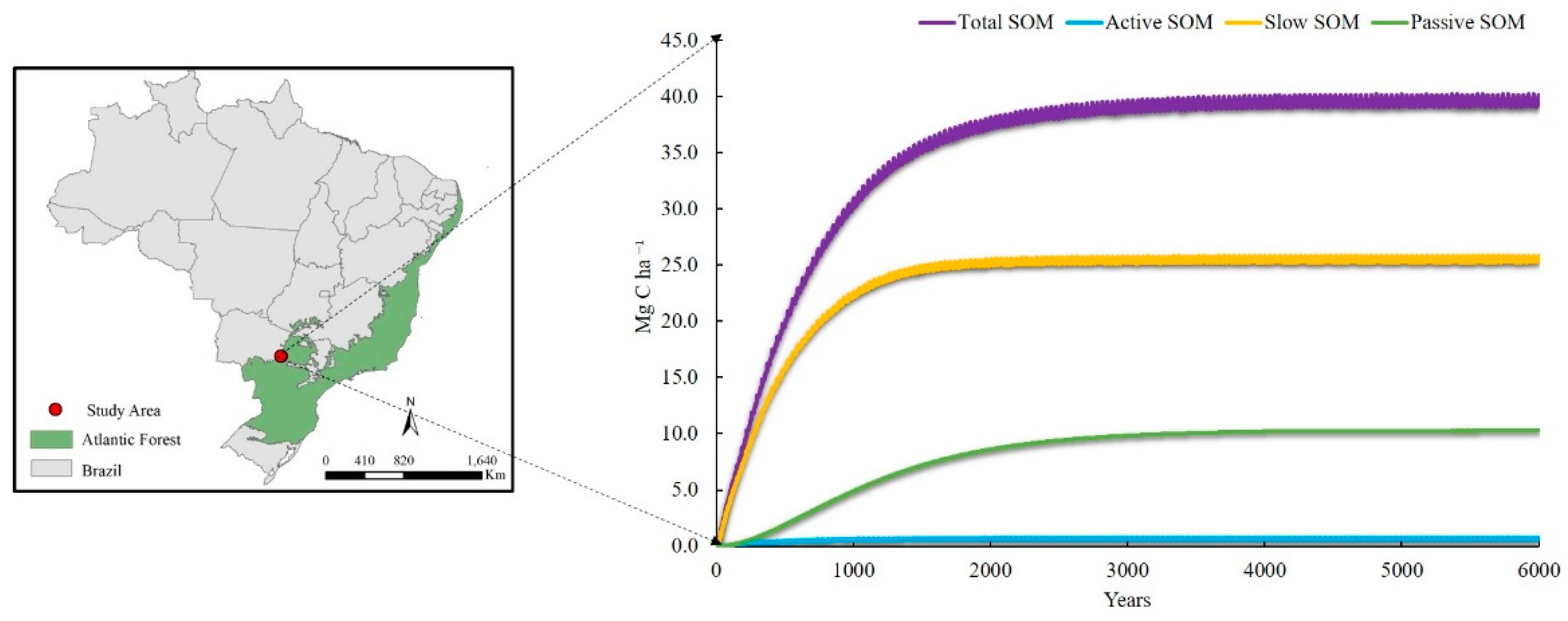
3.1. Equilibrium Modeling

The total simulated SOM was around 39.0 Mg C ha−1, where the major fraction was stored in Slow SOM, followed by the Passive SOM and a relatively small fraction in the Active SOM (Figure 5). The model suggested that SOM may take millennials to reach an equilibrium between the C addition and loss for the Atlantic Forest biome. The C stocks found for a native forest near the farm was reported as 36.4 Mg C ha−1, a difference of 6.7% compared to that simulated by DayCent (Figure 6).
For the simulations with the extensive pasture, in all paddocks in the study area in Caiuá, SP, the model calibration achieved good results because the values of total SOC measured in the literature compared their averages with a difference of 17.3% by DayCent (Figure 6).

3.2. Model Calibration

We considered the PRDX parameter in the mixed-pasture and soybean crop to achieve a refined calibration based on the observed values (Figure 7 and Table 2). For the first soybean cycle, the model responded well, while for the second soybean cycle and mixed-pasture, there were some paddocks (namely F3P4, F4P1, and F4P3) in which the model had a reasonable to poor response (Figure 7).
The parameters modified during equilibrium calibration, pre-experiment, and ICLS were considered using the range suggested by the DayCent manual (Table 2 and Table A3). The values of the parameters were estimated according to the literature; in the case of the C/N ratio, we used the changes in the PRAMX and PRAMN parameters (Table 2), following [63]. Plants with high N levels in their biomass, such as legumes, provide residues with a low C/N ratio, which means faster decomposition and, consequently, a higher N mineralization rate than other vegetables [63].
In the model calibration, the R2 for Aglivc was 0.69, which was statistically strong considering the observed data, with relative RMSE of 37.0%, MAE of 24.2%, and an NSE of 0.66 classified as satisfactory according to Moriasi [60] (Figure 8).

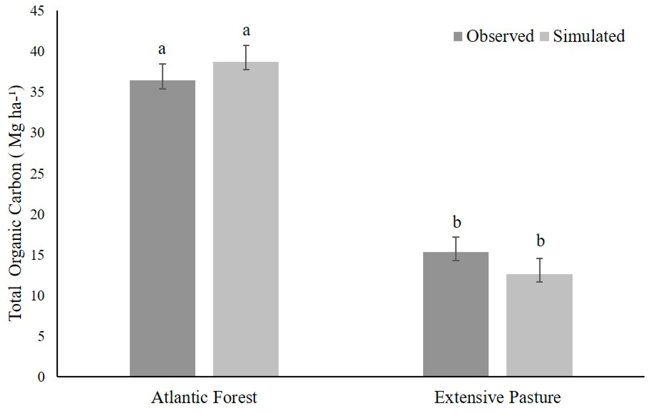
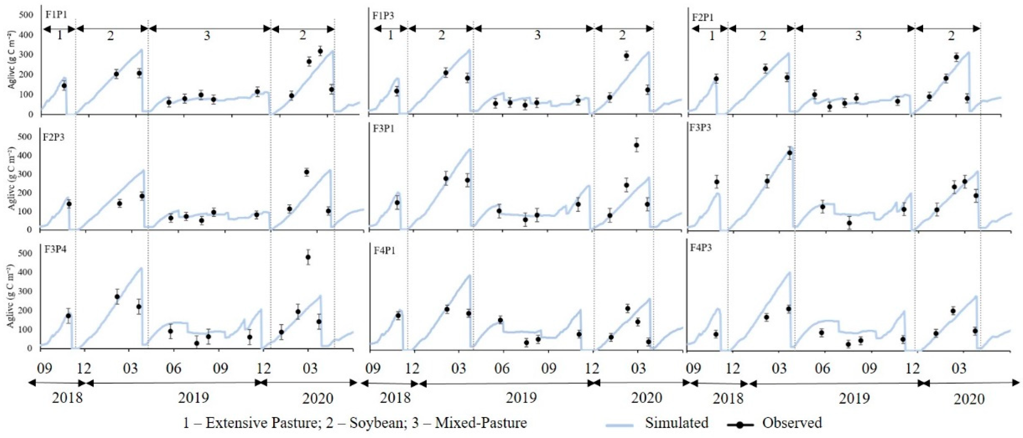
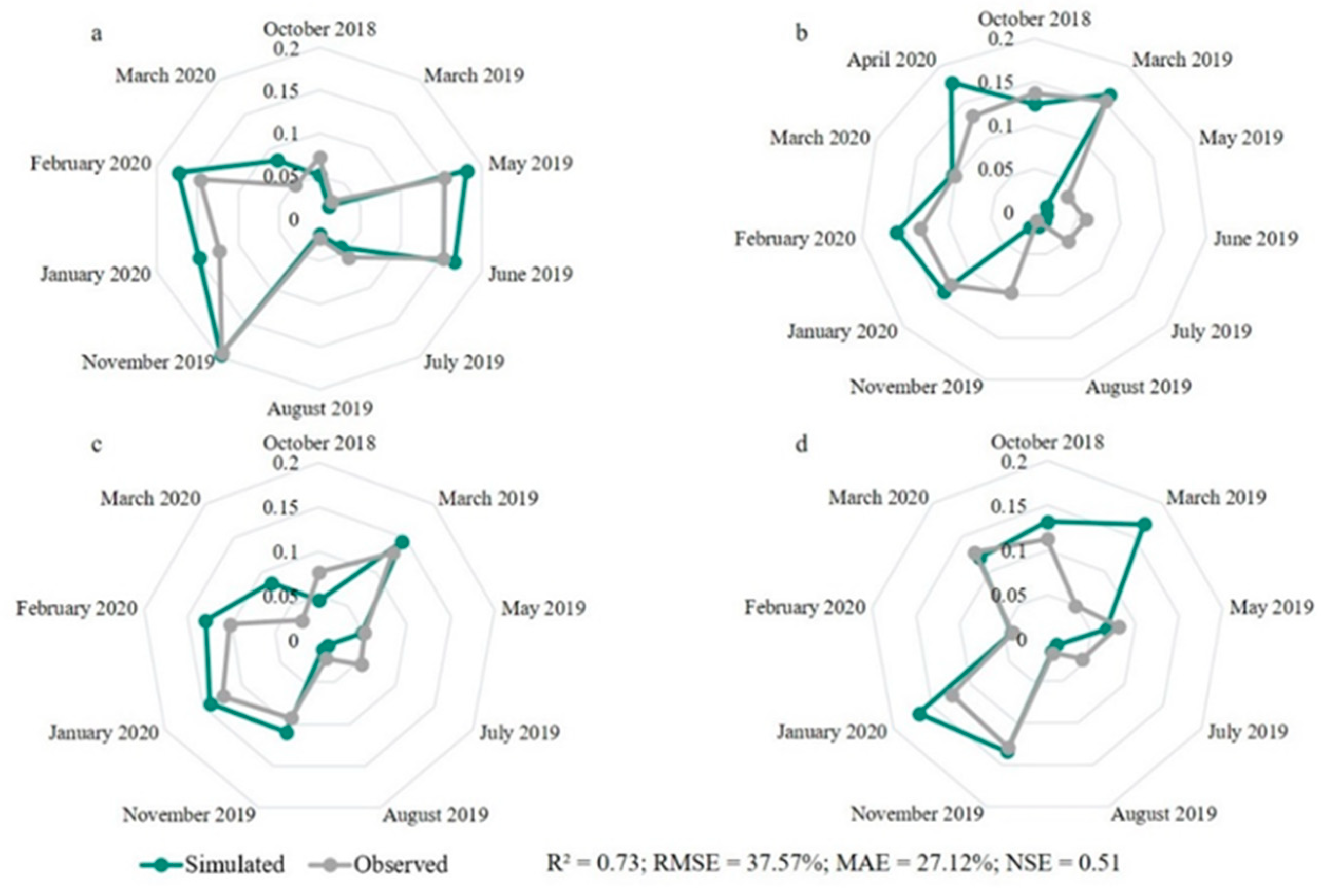
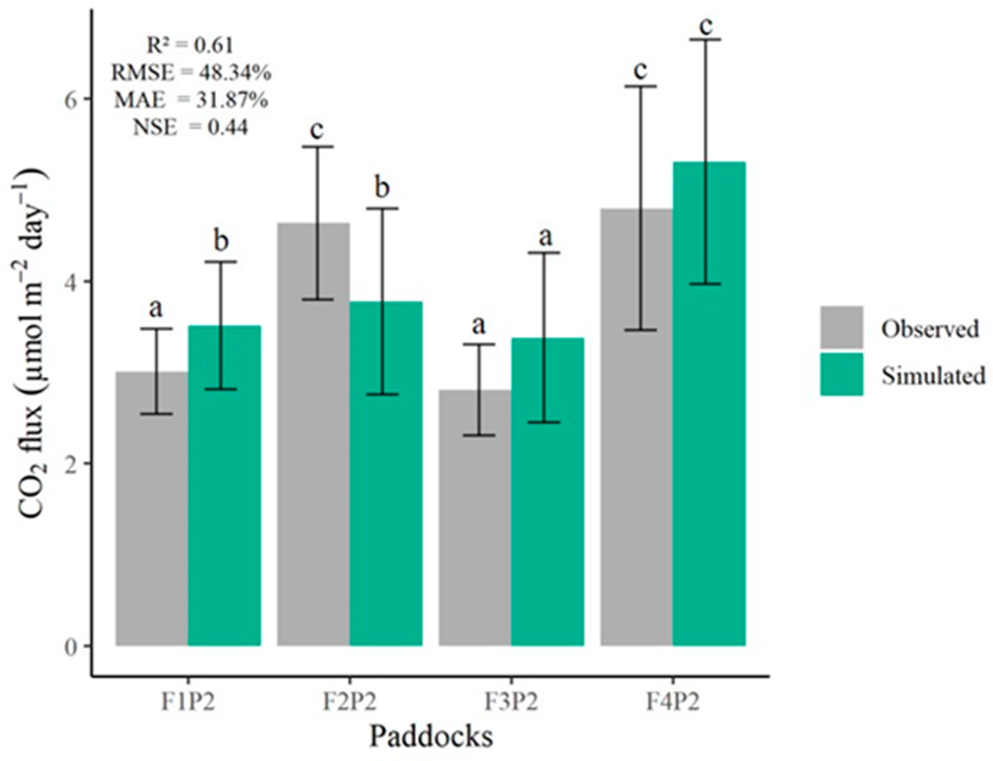
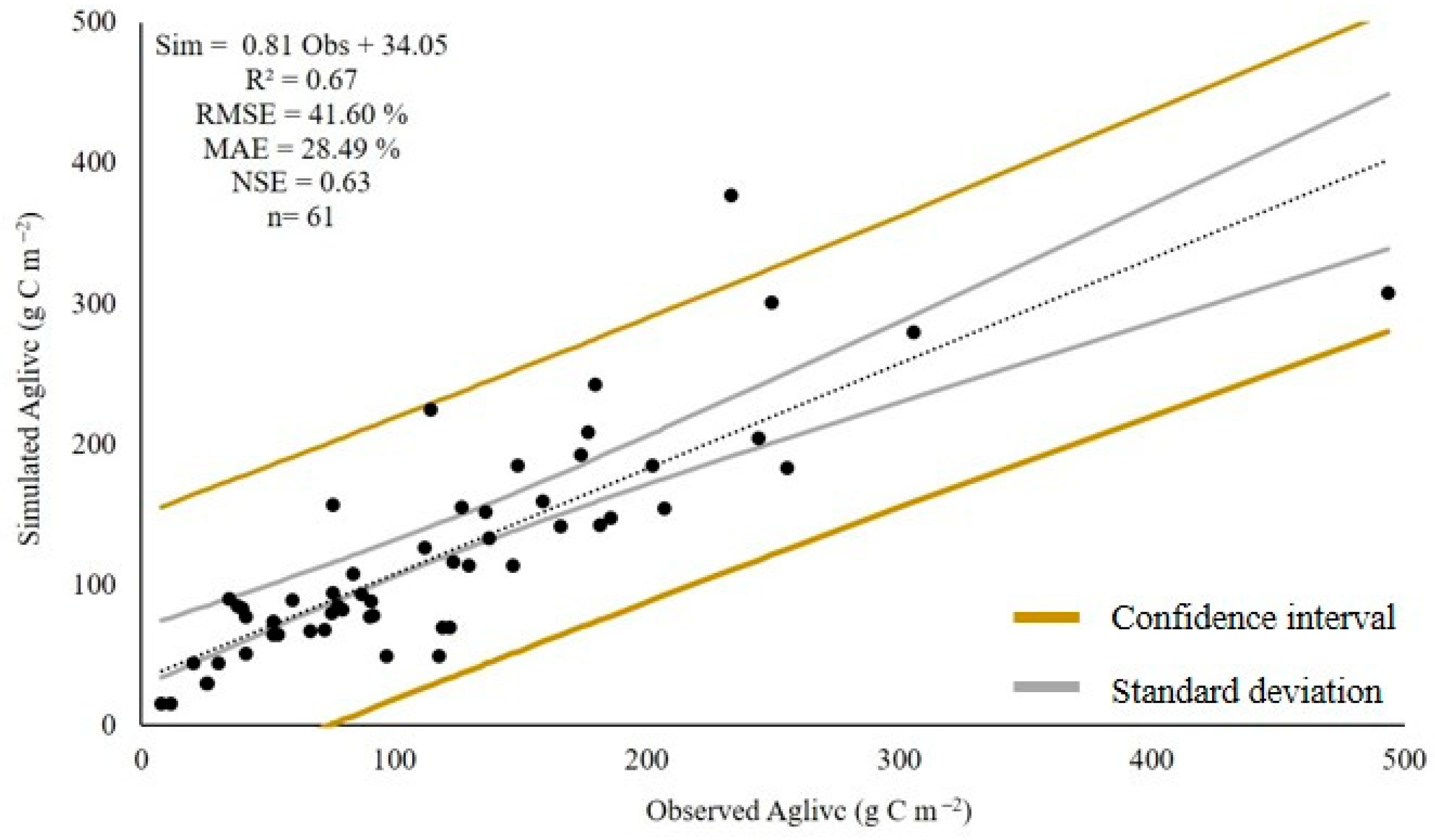
3.3. Model Validation

The model presented a consistent growth pattern along the seasons for the extensive pasture, before installing the ICLS, to the second soybean cycle and when the mixed-pasture was established (Figure 9). The mixed-pasture with values below 150 g C m−2, the vegetative peak of the first soybean cycle values above 300 g C m−2, and the second soybean, perhaps due to climatic factors, Aglivc was lower than the values of the first planting in the four paddocks.
The model captured the monthly variations in VWC and the variations between paddocks related to the soil sandy fraction variability and the crop management (cattle management between paddocks) after calibration, shown in Figure 10. Except for the F4P2 paddock (Figure 10d), all the others had similar behavior between simulated and observed during the study period yielding an R2 of 0.73, relative RMSE of 37.0%, MAE of 27.1%, and NSE of 0.51, indicating a good agreement (Figure 10b).
Regarding soil CO2 flux, the model overestimated three of the four paddocks used to validate such an agroecosystem variable. However, their average data were within the range of observed data during the ICLS (Figure 11). The lower NSE concerning the other analyzed parameters was 0.44, and relative RMSE was considered high at 48.3%, MAE of 31.9% and R2 of 0.61. By Tukey’s test, two of the four paddocks were considered to have equal means between simulated and observed (Figure 11).
In Figure 12, we brought together all Aglivc values from the validated paddocks and the two other regions (three ICLSs) to analyze how well the model responded to the observed values. For this generalized validation, model performance for Aglivc yielded R2 of 0.67, RMSE of 41.6%, and NSE of 0.63, indicating a good model fit.
We are considering a system with an output of two soybean cycles, one mixed-pasture cycle and the other data from farms that also used ICLS as a basis for mixed-pasture (Figure 12). The relative RMSE at 41.6%, MAE with 28.5%, and NSE with 0.63, we can consider as indicative of a low bias in the model, which was reinforced by visual analyzing of the convergence between the confidence interval line (gold) (95%) and the standard deviation (gray) with the regression line (observed vs. simulated) (Figure 12), with the majority of the simulated points falling within this confidence interval.
In the validation set, simulations of grain biomass (cgrain) presented similar average and quantiles’ values (Figure 13). The model was able to capture the variability among paddocks. Moreover, for the OR that the modeling was performed to prove the robustness of the model in ICLS, the model slightly overestimated the cgrain but represented well the variability. Tukey’s test indicated equal means for the four validated paddocks and OR, showing no significant difference between simulated and observed.

4. Discussion

4.1. Equilibrium

The replacement of natural ecosystems by agroecosystems with crops usually provides the decline in soil C content due to the reduction in the microbial C and the increase of SOM decomposition [64]. With the removal of the native vegetation and the beginning of the extensive pasture, the C stocks dropped in the soil (Figure 6). This may have been caused by the soil preparation (disturbing), breaking the aggregates offering protection to SOM and stimulating the biological activity [65].
In tropical ecosystems, the losses of C observed after the land clearing and cultivation of soils are more accelerated than in temperate regions [66]. Thus, the decrease of nutrients in an extensive pasture in native vegetation is due to soil revolving, even if minimal, since there is a negative effect on SOM [67,68,69]. Climatic conditions, especially temperature, also affect the decomposition rate of plant residues and the stabilization of SOM [44]. The occurrence of higher temperatures tends to accelerate the decomposition rate of SOM [70]. One alternative to increase the total C stock in the agriculture systems is by applying sustainable management practices and adopting crop systems that increase primary production and reduce C removal and soil degradation. Therefore, improved management practices affect the factors that regulate the synthesis and decomposition of SOM, contributing to the sustainable productivity of the ecosystem [71].

4.2. Calibrated Model

The DayCent model adequately simulated aboveground biomass (Figure 7), mainly for the beginning of the soybean crop and the mixed-pasture growth phases, periods that had no direct grazing effect on the simulations; even though it was an area with intensive pasture management, there were periods just after the mixed-pasture implementation where the animals were not present in some paddocks. All nine paddocks had the same altered parameters, and the behavior throughout the experiment was similar. Thus, minor model failures in predicting aboveground biomass did not influence each paddock’s overall behavior. Due to the study area being a commercial farm, minor problems with pests, diseases, and weeds may also have influenced the biomass production to some extent, all of which are not currently captured by the DayCent model unless we force the model to reproduce the reductions of potential plant growth.
Del Grosso et al. [22] reported that most of the errors in DayCent model outputs were associated with imperfections in model algorithms and parameters instead of uncertainty in model drivers. Therefore, efforts to improve the model should compare model outputs using numerous observations for various C and N components from field experiments to identify weaknesses and rectify model shortcomings [72].
There was no under- or overestimation tendency of the aboveground biomass simulations (Figure 8). The model explained 0.69 of the mixed-pasture, soybean, and extensive pasture measured data (Figure 8), which many authors found a 0.25–0.69 variation over aboveground biomass during the calibration stage [73].
In ICLS, there is a differentiated contribution of plant residues regarding conventional grain production systems, both in the surface and soil subsurface [74]. In intensive ICLS, the often succession of crop and pasture planting contributes to the root growth of both plants and potentially increases the SOM in the deeper soil layers [75]. SOM can be investigated by detailing its behavior over time in the future. Not only the inclusion of crops in pasture areas can contribute to improving the system, but also planting pastures in crop areas can increase crop yield by improving edaphic properties, the presence of straw and pasture roots, increasing C levels and significantly ameliorating the conditions of aeration and water infiltration capacity in the soil [76]. In future, we need to investigate the GHG mitigation which ICLS can potentially offer, which farmers can use to understand their carbon footprint, encouraging management strategies to improve agricultural sustainability [77].

4.3. Validated Model

In the validation stage, the DayCent model performed well in representing the ICLS, with the model results reflecting the dynamic phases of such a system (e.g., soybean replaced by mixed-pasture with a rotational and intensive grazing system) and management operations (e.g., sowing, harvesting, mowing, fertilization, grazing events) (Figure 7 and Figure 9). Even though three different soybean varieties were sowing in the area in both seasons, the model presented consistent aboveground biomass and yield simulation results. Perhaps the difference between the rainfall distribution and the difference in the average air temperature among cycles have not influenced the differentiation of aboveground biomass production.
For the four paddocks independently evaluated, the behavior of aboveground biomass shows that even with some differences, it was still possible to represent the ICLS (Figure 9). The model did not overestimate or underestimate aboveground biomass for the study period; previous studies have reported a DayCent tendency to underestimate grain yield and aboveground biomass [11,78,79]. Generally, significant errors may occur because the model does not consider several processes that depend on crop management, such as those associated with biotic stresses from weeds, diseases, or insects [80]. Additionally, improvements in the solving processes, such as replacing the generic phenology and partitioning rules by implementing traditional crop models such as the CROPGRO [81], could potentially overcome some of these challenges in predicting soybean development and growth and yields.
The DayCent model adequately simulated VWC (Figure 10) after adjustments during the calibration simulations. We highlight that the DayCent presents consistent results for these sand soils, similar to reported performance for other soil types in Brazil [82,83]. We had a median accuracy not only for the rainy season (December and January) but also for the driest months (July and August), unlike some studies that reported DayCent difficulties in simulating VWC in very dry periods [84], based on the reference described in Section 2.4.
The VWC and its dynamics are of utmost importance since it affects plant growth, SOM mineralization, and, therefore, the C fluxes in the model. Moreover, in crops such as soybean, water stress impacts not only direct the plant growth but also triggers morpho-physiological responses mainly in the reproductive phase, demonstrated by premature senescence of leaves and flowers, death of pods and, consequently, grain yield reduction [85]. Water stress effects on aboveground biomass (Figure 7 and Figure 9) and grain biomass (Figure 13) were noticed at some stages within the paddocks. In the DayCent modeling approach, these different species responses may be corrected by inserting different soil root distributions as model inputs, for example, adjusting the soil.in file (model input) to better represent the growth and distribution and add a water response factor in the crop.100 file to better represent crop response sensitivity to drought events. However, it is important to emphasize that these properties must be kept relatively constant for the same species. Their alteration must be based on quantifiable aspects of the production environments.
DayCent captured the highest observed values of CO2 emission linked to management events (Figure 11). The soil CO2 release occurs soon after the no-till practices. A few weeks later, when more C is incorporated into the soil, the broking of structures protecting C, make it available for the soil microorganisms. Consequently, more C is decomposed and released to the atmosphere, resulting, in the short term, in a reduction of the total SOC, and, if frequent, in the SOC content in the medium and longterm [86,87]. The flow of CO2 in the soil is very complex and incorporates both autotrophic and heterotrophic respiration and the passive diffusion of CO2, encompassing biological and physicochemical processes that control the CO2 fluxes into and out the soil, and between different C compartments of the soil system [88].
DayCent has received little assessment of CO2 predicted in tropical and ICLS conditions. As mentioned, this model was previously tested in Brazil in its capabilities to predict SOC changes [89], crop yield for common succession/rotation systems, N2O [15], and flows of CH4 [79], but not yet for CO2 fluxes, despite its importance in accurately simulating the conditions of a more intensive and complex system. DayCent overestimates the GHG over different environments [11,79,90], including our study. With an R2 of 0.61, and relative RMSE of 48.3%, when comparing the means, we only had differences in the F2P2 paddock, which can be explained by the plant residues having a higher C/N ratio and having a slower decomposition, thus staying longer in the ground, and the CO2 flux becomes lower than the others [91]. The results presented here show that CO2 flux can vary with the implementation of different ICLS, and depends on the management practices. Therefore, results support the importance of measuring and validating ecosystem models, such as DayCent, to predict the SOC and CO2 fluxes.
The validation for applications in OR showed consistent results (Figure 13). The simulated values were similar to those observed considering the two soybean crops. With a minimum precision error about the other parameters (relative RMSE = 11.3 %, MAE = 8.0 % and NSE = 0.52), we had a good result for DayCent within the ICLS for the soybean crop considering the adjusted model also for different sites. Study [92] found R2 = 0.32 for soybean, and in our validation, it was found at 0.61. Despite the dispersion, DayCent can estimate the productivity of various crops in different places in the world. This result suggests the model potential in estimating plant growth for monoculture systems, such as soybeans, and more complex systems, such as ICLS. The DayCent model considers abiotic influences on plant growth and development, such as solar incidence, temperature, and precipitation [86]. Thus, we expected that perfect coupling of the grain production estimated by the model would not occur (Figure 13).
A long-term ICLS implemented on sandy soil in a farm of western São Paulo state (SP) in Brazil, using a scheme of two years of soybean in the rainy season followed by pasture (dry season) and two years of only pasture, showed soybean yields ranging from 2.9 to 4.3 Mg ha−1, with the lowest values obtained under severe dry spells conditions [90]. These were considerably higher soybean yields than other farms in the same region in the conventional system (average of 1.8 Mg ha−1) [93], indicating that the increment in agricultural outputs may benefit from ICLSs.
We found similar performance for the ICLS in our area and for the other three regions (Figure 12) as previously reported for other pasture species (R2 = 0.67) [94]. Although the results suggest that the model can predict an ICLS, additional validations are needed due to the diversity of ICLS and its adoption over different production environments, such as cultivated species, animals raised, soil textures and classes, climates, and management practises. This is a fundamental step for any model application beyond the environmental conditions that the model was evaluated, to check how stable the calibration is and to what extent the model can be extrapolated.
The study area benefited from the adoption of the ICLS by deciding to replace a degraded pasture and adopt this system. The system creates a synergy between soybean-pasture-soybean, being beneficial for both monoculture and mixed-pasture, and helps increase soil nutrients, improving land-use diversification based on the spatial and temporal integration of crop and livestock components. The result can reduce pressure to open new areas for production, proving to be an excellent option for sustainable food production. However, gaps in knowledge about the long-term effects of ICLS can make it difficult for farmers to evaluate the benefits that ICLS may provide to their farm production and impose a barrier to payments for environmental services, such as carbon credits [95]. By properly modeling ICLS, the long-term effect can be accounted for contributing with positive credits in the C trading or even participating in traceability regarding the sustainability within the beef cattle market.

5. Conclusions

In this study, we calibrated and validated the DayCent model in ICLS farms in tropical Brazil, particularly over sandy soils. With the simulation of two pastures grown simultaneously, it was possible to fill in a gap that had not yet been addressed with DayCent, especially when using a system as complex and intense as the ICLS which we analyzed in our study. By using the aboveground biomass data to calibrate DayCent parameters, it was demonstrated that the model could be simplified according to the amount of data available, and it was possible to simulate plant growth, grain biomass, soil VWC, total SOC and CO2 fluxes, considering spatio-temporal evaluation and precision and accuracy metrics. Consistent simulations of grain biomass and plant growth data for other ICLSs were also found. Our study is an important step towards understanding the benefits of ICLSs and future regional analyses of the large-scale impacts of new agricultural practices, particularly over tropical environments.

Author Contributions

Conceptualization, Y.F.S., R.V.V., H.B.D., S.V.C., E.E.C., R.B. and G.K.D.A.F.; methodology, Y.F.S., R.V.V., H.B.D., S.V.C., E.E.C. and G.K.D.A.F.; software, Y.F.S., R.V.V. and E.E.C.; validation, Y.F.S. and R.V.V.; formal analysis, Y.F.S.; investigation, Y.F.S. and R.V.V.; resources, Y.F.S., E.M. and P.S.G.M.; data curation, Y.F.S.; writing—original draft preparation, Y.F.S., R.V.V., E.E.C. and G.K.D.A.F.; writing—review and editing, Y.F.S., R.V.V., H.B.D., S.V.C., E.E.C., R.A.C.L., E.M., R.B., M.R.A., P.S.G.M. and G.K.D.A.F.; visualization, Y.F.S., R.V.V.; supervision, S.V.C., E.E.C., R.A.C.L., E.M., P.S.G.M. and G.K.D.A.F.; project administration, E.E.C. and G.K.D.A.F.; funding acquisition, P.S.G.M. All authors have read and agreed to the published version of the manuscript.

Funding

This research was funded by CNPq (Process number 167705/2018-0) and FAPESP (Process numbers 2017/50205-9, 2018/24707-0, and 2020/06775-8).

Institutional Review Board Statement

Not applicable.

Informed Consent Statement

Not applicable.

Data Availability Statement

Acknowledgments

The authors would like to thank the owner, manager, and staff of the Campina farm (CV Nelore Mocho) for their support and assistance. We are also grateful to the undergraduate and graduate students, postdoctoral researchers, and also to the technicians for helping with the field data collection and preparation. NIPE and FEAGRI/UNICAMP are acknowledged for the infrastructure and support provided for this project development. Meteorological data were obtained from the NASA Langley Research Center (LaRC) POWER Project funded through the NASA Earth Science/Applied Science Program.

Conflicts of Interest

The authors declare no conflict of interest.

Appendix A

Table A1. Management information of each paddock (pad.) within-season and off-season phases for ICLS.
Season Managements (Crop Phase)
Soybean Cycle 2018/2019Soybean Cycle 2019/2020
FieldPad.CultivarSowing dateHarvest dateCultivarSowing dateHarvest date
11, 2, 3BRS7380 RR18 November 201802 April 2019NS670012 December 201907 April 2020
21, 2, 3AS3730 IPRO20 November 201830 March 2019NS670011 December 201904 April 2020
31, 2, 3, 4NS670021 November 201804 April 2019AS3730 IPRO13 December 201908 April 2020
41, 2, 3NS670022 November 201805 April 2019BRS7380 RR15 December 201909 April 2020
Off-season managements in 2019 (mixed-pasture phase)
FieldPad.Mixed-pastureSowing date1° Grazing2° Grazing3° GrazingEvents
PeriodStocking ratePeriodStocking ratePeriodStocking rateMowing
11Millet + ruzigrass02/0417/05–26/0515214/07–21/075917/08–28/0810315/06
226/05–04/0621/07–28/0728/08–08/09
304/06–12/0628/07–03/0808/09–20/09
21Millet + ruzigrass04/0417/05–25/0520514/07–21/075717/08–28/0810314/06
225/05–02/0621/07–28/0728/08–08/09
302/06–09/0628/07–03/0808/09–20/09
31Millet + ruzigrass05/0427/05–07/0614617/08–26/0814309/10–14/10121-
207/06–18/0626/08–05/0914/10–19/10
318/06–29/0605/09–14/0919/10–24/10
429/06–11/0714/09–22/0924/10–31/10
41Millet + ruzigrass06/0431/05–14/0616317/08–29/0878---
214/06–28/0629/08–10/09
328/06–11/0710/09–22/09
Table A2. Sampling fields collects periods and data from ICLS on study area.
Sampling Fields Collects Period Land UseSystem PhaseCollected DataSampled Fields
28 October 2018Extensive pasture Before ICLSSoil samplings for determination of soil organic carbon and pH, aboveground biomass, volumetric soil water content, bulk density, total soil carbon1, 2, 3, 4
5 February 2019Soybean ICLSAboveground biomass, volumetric soil water content 1, 2, 3, 4
21 March 2019Soybean ICLSAboveground biomass, volumetric soil water content, grain biomass1, 2, 3, 4
18 April 2019Mixed-pasture ICLSSoil respiration1, 2, 3, 4
01 May 2019Mixed-pasture ICLSSoil respiration1, 2, 3, 4
11 May 2019Mixed-pasture ICLSSoil respiration1, 2, 3, 4
17 May 2019Mixed-pastureICLSAboveground biomass, volumetric soil water content 1 and 2
25 May 2019Mixed-pasture ICLSAboveground biomass, volumetric soil water content 3 and 4
16 June 2019Mixed-pasture ICLSAboveground biomass, volumetric soil water content1 and 2
17 July 2019Mixed-pasture ICLSAboveground biomass, volumetric soil water content1, 2, 3, 4
10 August 2019Mixed-pasture ICLSAboveground biomass, volumetric soil water content1, 2, 3, 4
2 November 2019Mixed-pasture ICLSAboveground biomass, volumetric soil water content1, 2, 3, 4
8 November 2019Mixed-pasture ICLSSoil respiration1, 2, 3
15 November 2019Mixed-pasture ICLSSoil respiration1, 2, 3, 4
6 January 2020Soybean ICLSAboveground biomass, volumetric soil water content1, 2, 3, 4
8 January 2020SoybeanICLSSoil respiration1, 2, 3, 4
9 February 2020Soybean ICLSAboveground biomass, volumetric soil water content1, 2, 3, 4
14 February 2020SoybeanICLSSoil respiration1, 2, 3, 4
1 March 2020Soybean ICLSAboveground biomass, volumetric soil water content1, 2, 3, 4
1 March 2020SoybeanICLSSoil respiration1, 2, 3
23 March 2020Soybean ICLSAboveground biomass, volumetric soil water content, grain biomass1, 2, 3, 4
23 March 2020SoybeanICLSSoil respiration1, 2, 3, 4
Table A3. The description about the modified parameters used in the DayCent model.
InitialsDescriptions
AGLREMFraction of aboveground live which will not be affected by harvest operations
BGLREMFraction of belowground live which will not be affected by harvest operations
BIOMAXAboveground biomass level above which the minimum and maximum C/E ratios of new shoot increments equal pramn(*,2) and pramx(*,2), respectively
CLAYPGNumber of soil layers that crop roots can occupy. The value used as CLAYPG for annual plants will vary from 1 on the day that plant growth starts to CLAYPG as read from the CROP option on day FRTC(3) of plant growth
EFRGRN(1)Fraction of aboveground N which goes to grain
FDGREMFraction of standing dead (stdedc) removed by a grazing event over a one-month period. The daily removal rate is approximately fdgrem/30
FERAMT(1)Amount of N to be added
FERAMT(2)Amount of P to be added
FLGREMFraction of live shoots (aglivc) removed by a grazing event over a one-month period. The daily removal rate is approximately flgrem/30
FULCANValue of aboveground live C (aglivc) at full canopy cover, above which potential production is not reduced (above which there is no restriction on seedling growth)
PPDF(3)Left curve shape for parameterization of a Poisson Density Function curve to simulate temperature effect on growth
PPDF(4)Right curve shape for parameterization of a Poisson Density Function curve to simulate temperature effect on growth
PRAMN(1,1)Minimum aboveground C/N ratio with zero biomass
PRAMN(1,2)Minimum aboveground C/N ratio with biomass > biomax
PRAMX(1,1)Maximum aboveground C/N ratio with zero biomass
PRAMX(1,2)Maximum aboveground C/N ratio with biomass > biomax
PRDX(1)Coefficient for calculating total monthly potential production as a function of solar radiation outside the atmosphere. It functions as a radiation use efficiency scalar on potential production. It reflects the relative genetic potential of the plant; larger PRDX(1) values indicate greater growth potential
PRDX(2)Coefficient for calculating total monthly potential production as a function of solar radiation outside the atmosphere. It functions as a radiation use efficiency scalar on potential production. It reflects the relative genetic potential of the plant; larger PRDX(2) values indicate greater growth potential
SNFXMXMaximum symbiotic N fixation for forest (actual symbiotic N fixation will be less if available mineral N is sufficient for growth)
Figure A1. Meteorological data of the other regions where the DayCent simulations were performed ((a)—Dourado; (b)—São Gabriel do Oeste; (c)—Rondonopolis) and also the historical average climate of the reference area of native vegetation in Presidente Prudente (d).
Sustainability 14 03517 g0a1

References

  1. Moraes, A.; Carvalho, P.C.F.; Anghinoni, I.; Lustosa, S.B.C.; Costa, S.E.V.G.A.; Kunrath, T.R. Integrated crop—Livestock systems in the Brazilian subtropics. Eur. J. Agron. 2014, 57, 4–9. [Google Scholar] [CrossRef]
  2. Embrapa. ILPF em Número, 12. 2016. Available online: https://ainfo.cnptia.embrapa.br/digital/bitstream/item/158636/1/2016-cpamt-ilpf-em-numeros.pdf (accessed on 1 August 2021). (In Portuguese).
  3. Bonaudo, T.; Bendahan, A.B.; Sabatier, R.; Ryschawy, J.; Bellon, S.; Leger, F.; Magda, D.; Tichit, M. Agroecological principles for the redesign of integrated crop-livestock systems. Eur. J. Agron. 2014, 57, 43–51. [Google Scholar] [CrossRef]
  4. Wruck, F.J.; Behling, M.; Antonio, D.B.A. Sistemas Integrados em Mato Grosso e Goiás. In Sistemas Agroflorestais: A Agropecuária Sustentável, 1st ed.; Alves, F.V., Laura, V.A., Almeida, R.G., Eds.; Embrapa: Brasilia, Brazil, 2015; pp. 169–194. (In Portuguese) [Google Scholar]
  5. Silva, L.S.; Laroca, J.V.S.; Coelho, A.P.; Gonçalves, E.C.; Gomes, R.P.; Pacheco, L.P.; Carvalho, P.C.F.; Pires, G.C.; Oliveira, R.L.; Souza, J.M.A.; et al. Does grass-legume intercropping change soil quality and grain yield in integrated crop-livestock systems? Appl. Soil Ecol. 2022, 170, 104257. [Google Scholar] [CrossRef]
  6. Jones, J.W.; Hoogenboom, G.; Porter, C.H.; Boote, K.J.; Batchelor, W.D.; Hunt, L.A.; Wilkens, P.W.; Singh, U.; Gijsman, A.J.; Ritchie, J.T. The DSSAT cropping system model. Eur. J. Agron. 2003, 18, 3–4. [Google Scholar] [CrossRef]
  7. Zhang, Y.; Hansen, N.; Trout, T.; Nielsen, D.; Paustian, K. Modeling Deficit Irrigation of Maize with the DayCent Model. Agron. J. 2018, 110, 1754–1764. [Google Scholar] [CrossRef]
  8. Nehbandani, A.; Soltani, A.; Hajjarpoor, A.; Dadrasi, A.; Nourbakhsh, F. Comprehensive yield gap analysis and optimizing agronomy practices of soybean in Iran. J. Agric. Sci. 2020, 158, 739–747. [Google Scholar] [CrossRef]
  9. Zhang, Y.; Gurung, R.; Marx, E.; Williams, S.; Ogle, S.M.; Paustian, K. DayCent model predictions of NPP and grain yields for agricultural lands in the contiguous U.S. J. Geophys. Res. Biogeosci. 2020, 125, e2020JG005750. [Google Scholar] [CrossRef]
  10. Lemma, B.; Williams, S.; Paustian, K. Long term soil carbon sequestration potential of smallholder croplands in southern Ethiopia with Daycent model. J. Environ. Manag. 2021, 294, 112893. [Google Scholar] [CrossRef]
  11. Necpálová, M.; Anex, R.P.; Fienen, M.N.; Del Grosso, S.J.; Castellano, M.J.; Sawyer, J.E.; Iqbal, J.; Pantoja, J.L.; Barker, D.W. Understanding the Daycent model: Calibration, sensitivity, and identifiability through inverse modeling. Environ. Model. Softw. 2015, 66, 110–130. [Google Scholar] [CrossRef] [Green Version]
  12. Frolking, S.E.; Moiser, A.R.; Ojima, D.S.; Li, C.; Parton, W.J.; Potter, C.S.; Priesack, E.; Stenger, R.; Haberbosch, C.; Dorsch, P. Comparison of N2O Emissions from Soils at Three Temperate Agricultural Sites: Simulations of year-round measurements by four models. Nutr. Cycl. Agroecosyst. 1998, 52, 77–105. [Google Scholar] [CrossRef]
  13. Del Grosso, S.J.; Mosier, A.R.; Parton, W.J.; Ojima, D.S. Daycent model analysis of past and contemporary soil N2O and net greenhouse gas flux for major crops in the USA. Soil Tillage Res. 2005, 83, 9–24. [Google Scholar] [CrossRef]
  14. Parton, W.J.; Hartman, M.; Ojima, D.; Schimel, D. Daycent description and testing. Glob. Planet. Chang. 1998, 19, 35–48. [Google Scholar] [CrossRef]
  15. Weiler, D.A.; Tornquist, C.G.; Parton, W.; Santos, H.P.; Santi, A.; Bayer, C. Crop Biomass, Soil Carbon, and Nitrous Oxide as Affected by Management and Climate: A Daycent Application in Brazil. Soil Sci. Soc. Am. J. 2017, 81, 945–955. [Google Scholar] [CrossRef]
  16. Damian, J.M.; Matos, E.S.; Pedreira, B.C.; Carvalho, P.C.F.; Premazzi, L.M.; Williams, S.; Paustian, K.; Cerri, C.E.P. Predicting soil C changes after pasture intensification and diversification in Brazil. Catena 2021, 202, 105238. [Google Scholar] [CrossRef]
  17. Laroca, J.V.S.; Souza, J.M.A.; Pires, G.C.; Pires, G.J.C.; Pacheco, L.P.; Silva, F.D.; Wruck, F.J.; Carneiro, M.A.C.; Silva, L.S.; Souza, E.D. Soil quality and soybean productivity in crop-livestock integrated system in no-tillage. Pesqui. Agropecu. Bras. 2018, 53, 1248–1258. [Google Scholar] [CrossRef]
  18. FAO. Measuring and Modelling Soil Carbon Stocks and Stock Changes in Livestock Production Systems. 2018. Available online: http://www.fao.org/3/I9693EN/i9693en.pdf (accessed on 15 September 2021).
  19. Fitton, N.; Bindi, M.; Brilli, L.; Cichota, R.; Dibari, C.; Fuchs, K.; Huguenin-elie, O.; Klumpp, K.; Lieffering, M.; Lüscher, A.; et al. Modelling biological N fixation and grass-legume dynamics with process-based biogeochemical models of varying complexity. Eur. J. Agron. 2019, 106, 58–66. [Google Scholar] [CrossRef]
  20. Baslam, M.; Mitsui, T.; Hodges, M.; Priesack, E.; Herritt, M.T.; Aranjuelo, I.; Sanz-Sáez, Á. Photosynthesis in a changing global climate: Scaling up and scaling down in crops. Front. Plant Sci. 2020, 11, 882. [Google Scholar] [CrossRef]
  21. Keohane, N.; Petsonk, A.; Hanafi, A. Toward a club of carbon markets. Clim. Chang. 2015, 144, 81–95. [Google Scholar] [CrossRef] [Green Version]
  22. Del Grosso, S.J.; Parton, W.J.; Adler, P.R.; Davis, S.C.; Keough, C.; Marx, E. Daycent model simulations for estimating soil carbon dynamics and greenhouse gas fluxes from agricultural production systems. In Managing Agricultural Greenhouse Gases; Elsevier Inc.: Amsterdam, The Netherlands, 2012; pp. 241–250. [Google Scholar]
  23. Hartman, M.; Parton, W.; Del Grosso, S.; Easter, M.; Hendryx, J.; Hilinski, T.; Kelly, R.; Keough, C.; Killian, K.; Lutz, S.; et al. The Daily Century Ecosystem, Soil Organic Matter, Nutrient Cycling, Nitrogen Trace Gas, and Methane Model: User Manual, Scientific Basis, and Technical Documentation. In Natural Resource Ecology Laboratory; Colorado State University: Fort Collins, CO, USA, 2018. [Google Scholar]
  24. United Nations General Assembly. Transforming Our World: The 2030 Agenda for Sustainable Development. 2015. Available online: http://www.un.org/ga/search/view_doc.asp?symbol=A/RES/70/1&Lang=E (accessed on 20 January 2022).
  25. Gil, J.D.B.; Reidsma, P.; Giller, K.; Todman, L.; Whitmore, A.; Van Ittersum, M. Sustainable development goal 2: Improved targets and indicators for agriculture and food security. Ambio 2019, 48, 685–698. [Google Scholar] [CrossRef] [Green Version]
  26. Campbell, B.M.; Hansen, J.; Rioux, J.; Stirling, C.M.; Twomlow, S.; Wollenberg, E.L. Urgent action to combat climate change and its impacts (SDG 13): Transforming agriculture and food systems. Curr. Opin. Environ. Sustain. 2018, 34, 13–20. [Google Scholar] [CrossRef]
  27. UN. SDG-15; Life on Land: Why It Matters. United Nations Sustainable Development Goals: New York, NY, USA, 2016.
  28. Rolim, G.S.; Camargo, M.B.P.; Grosselilania, D.; Moraes, J.F.L. Climatic classification of Köppen and Thornthwaite sistems and their applicability in the determination of agroclimatic zonning for the state of São Paulo, Brazil. Bragantia 2007, 66, 711–720. [Google Scholar] [CrossRef] [Green Version]
  29. Battisti, R.; Bender, F.D.; Sentelhas, P.C. Assessment of different gridded weather data for soybean yield simulations in Brazil. Theor. Appl. Climatol. 2019, 135, 237–247. [Google Scholar] [CrossRef]
  30. Dias, H.B.; Sentelhas, P.C. Assessing the performance of two gridded weather data for sugarcane crop simulations with a process-based model in Center-South Brazil. Int. J. Biometeorol. 2021, 65, 1881–1893. [Google Scholar] [CrossRef]
  31. Bender, F.D.; Sentelhas, P.C. Solar Radiation Models and Gridded Databases to Fill Gaps in Weather Series and to Project Climate Change in Brazil. Adv. Meteorol. 2018, 2018, 6204382. [Google Scholar] [CrossRef] [Green Version]
  32. Folfaro, V.J.; Neto, F.S. Ensaio de caracterização estratigrafica do cretaceo no estado de São Paulo: Grupo bauru. Rev. Bras. Geociênc 1976, 10, 177–185. (In Portuguese) [Google Scholar]
  33. Moniz, A.C.; Carvalho, A. Sequência de evolução de solos derivados do arenito Bauru e de rochas básicas da região noroeste do estado de São Paulo. Bragantia 1973, 32, 309–335. (In Portuguese) [Google Scholar] [CrossRef]
  34. Rossi, M. Mapa Pedológico do Estado de São Paulo: Revisado e Ampliado; Instituto Florestal: Sao Paulo, Brazil, 2017. (In Portuguese)
  35. Schoeneberger, P.; Wysocki, D.; Busskohl, C.; Libohova, Z. Landscapes, Geomorphology, and Site Description; USDA Natural Resources Conservation Service Soils: Waverley, IA, USA, 2017; Volume 18, pp. 21–80.
  36. Esquerdo, J.C.D.M.; Antunes, J.F.G.; Coutinho, A.C.; Speranza, E.A.; Kondo, A.A.; Santos, J.L. SATVeg: A web-based tool for visualization of MODIS vegetation indices in South America. Comput. Electron. Agric. 2020, 175, 105516. [Google Scholar] [CrossRef]
  37. Sato, A.; Tsuyuzaki, T.; Seto, M. Effect of Soil Agitation, Temperature or Moisture on Microbial Biomass Carbon of a Forest and an Arable Soil. Microbes Environ. 2000, 15, 23–30. [Google Scholar] [CrossRef] [Green Version]
  38. Embrapa. Manual de Métodos de Análise de Solo; Embrapa CNPS: Rio de Janeiro, Brazil, 1997. (In Portuguese) [Google Scholar]
  39. FAO. Knowledge Reference for National Forest Assessments—Modeling for Estimation and Monitoring. 2005. Available online: http://www.fao.org/forestry/17111/en/ (accessed on 15 September 2021).
  40. Rigolin, I.M.; Santos, C.H.; Calonego, J.C.; Tiritan, C.S. Estoque De Carbono Do Solo Em Sistemas Vegetais Com Manejo Agrícola Diferenciado No Oeste Paulista. Colloq. Agrar. 2013, 9, 16–29. (In Portuguese) [Google Scholar] [CrossRef]
  41. Souza, M.C. Consorciação de braquiária, milheto e crotalária em safrinha na produção de fitomassa e cobertura do solo. In 35 f. Trabalho de Conclusão de Curso (Graduação em Engenharia Agrícola e Ambiental); Universidade Federal de Mato Grosso, Instituto de Ciências Agrárias e Tecnológicas: Rondonopolis, Brazil, 2018. (In Portuguese) [Google Scholar]
  42. Machado, L.A.Z. Misturas de forrageiras anuais e perenes para sucessão à soja em sistemas de integração lavoura pecuária. Pesqui. Agropecu. Bras. 2012, 47, 629–636. (In Portuguese) [Google Scholar] [CrossRef] [Green Version]
  43. Del Grosso, S.J.; Parton, W.J.; Mosier, A.R.; Hartman, M.D.; Brenner, J.; Ojima, D.S.; Schimel, D.S. Simulated interaction of carbon dynamics and nitrogen trace gas fluxes using the Daycent model. In Modeling Carbon and Nitrogen Dynamics for Soil Management; Schaffer, M., Ma, L., Hansen, S., Eds.; CRC Press: Boca Raton, FL, USA, 2001; pp. 303–332. [Google Scholar]
  44. Parton, W.J.; Schimel, D.S.; Cole, C.V.; Ojima, D.S. Analysis of factors controlling soil organic levels of grasslands in the Great Plains. Soil Sci. Soc. Am. J. 1987, 51, 1173–1179. [Google Scholar] [CrossRef]
  45. Parton, W.J.; Stewart, J.W.B.; Cole, C.V. Dynamics of C, N, P and S in grassland soils: A model. Biogeochemistry 1988, 5, 109–131. [Google Scholar] [CrossRef]
  46. Wieder, W.R.; Hartman, M.D.; Sulman, B.N.; Wang, Y.-P.; Koven, C.D.; Bonan, G.B. Carbon cycle confidence and uncertainty: Exploring variation among soil biogeochemical models. Glob. Chang. Biol. 2018, 24, 1563–1579. [Google Scholar] [CrossRef] [Green Version]
  47. Saxton, K.E.; Rawls, W.J.; Romberger, J.S.; Papendick, R.I. Estimating generalized soil-water characteristics from texture. Soil Sci. Soc. Am. J. 1986, 50, 1031–1036. [Google Scholar] [CrossRef]
  48. Garrison, M.V.; Batchelor, W.D.; Kanwar, R.S.; Ritchie, J.T. Evaluation of the CERES-Maize water and nitrogen balances under tile-drained conditions. Agric. Syst. 1999, 62, 189–200. [Google Scholar] [CrossRef]
  49. Chen, L.; Wang, K.; Baoyin, T. Effects of grazing and mowing on vertical distribution of soil nutrients and their stoichiometry (C:N:P) in a semi-arid grassland of North China. Catena 2021, 206, 105507. [Google Scholar] [CrossRef]
  50. Gilmullina, A.; Rumpel, C.; Blagodatskaya, E.; Chabbi, A. Management of grasslands by mowing versus grazing—Impacts on soil organic matter quality and microbial functioning. Appl. Soil Ecol. 2020, 156, 103701. [Google Scholar] [CrossRef]
  51. Heggenstaller, A.H.; Moore, K.J.; Liebman, M.; Anex, R.P. Nitrogen influences biomass and nutrient partitioning by perennial, warm-season grasses. Agron. J. 2009, 101, 1363–1371. [Google Scholar] [CrossRef]
  52. Sainju, U.M.; Allen, B.L.; Lenssen, A.W.; Ghimire, R.P. Root biomass, root/shoot ratio, and soil water content under perennial grasses with different nitrogen rates. Field Crop. Res. 2017, 210, 183–191. [Google Scholar] [CrossRef] [Green Version]
  53. Zhang, F.; Wang, Q.; Hong, J.; Chen, W.; Qi, C.; Ye, L. Life cycle assessment of diammonium-and monoammonium-phosphate fertilizer production in China. J. Clean. Prod. 2017, 141, 1087–1094. [Google Scholar] [CrossRef]
  54. Anghinoni, G.; Anghinoni, F.B.G.; Tormena, C.A.; Braccini, A.L.; Mendes, I.C.; Zancanaro, L.; Lal, R. Conservation agriculture strengthen sustainability of Brazilian grain production and food security. Land Use Policy 2021, 108, 105591. [Google Scholar] [CrossRef]
  55. Soares, D.S.; Ramos, M.L.G.; Marchão, R.L.; Maciel, G.A.; Oliveira, A.D.; Malaquias, J.V.; Carvalho, A.M. How diversity of crop residues in long-term no-tillage systems affect chemical and microbiological soil properties. Soil Tillage Res. 2019, 194, 104316. [Google Scholar] [CrossRef]
  56. Nascente, A.S.; Li, Y.C.; Crusciol, C.A.C. Cover crops and no-till effects on physical fractions of soil organic matter. Soil Tillage Res. 2013, 130, 52–57. [Google Scholar] [CrossRef]
  57. Teixeira, R.A.; Soares, T.G.; Fernandes, A.R.; Braz, A.M.S. Grasses and legumes as cover crop in no-tillage system in northeastern Pará Brazil. Acta Amaz. 2014, 44, 411–418. [Google Scholar] [CrossRef]
  58. Yang, J.M.; Yang, J.Y.; Liu, S.; Hoogenboom, G. An evaluation of the statistical methods for testing the performance of crop models with observed data. Agric. Syst. 2014, 127, 81–89. [Google Scholar] [CrossRef]
  59. Priesack, E.; Gayler, S.; Hartmann, H. The impact of crop growth sub-model choice on simulated water and nitrogen balances. Nutr. Cycl. Agroecosyst. 2006, 75, 1–13. [Google Scholar] [CrossRef]
  60. Moriasi, D.N.; Arnold, J.G.; Liew, M.W.V.; Bingner, R.L.; Harmel, R.D.; Veith, T.L. Model evaluation guidelines for systematic quantification of accuracy in watershed simulations. ASABE 2007, 50, 885–900. [Google Scholar] [CrossRef]
  61. Ihaka, R. Gentleman R: A language for data analysis and graphics. J. Comput. Graph. Stat. 1996, 5, 299–314. [Google Scholar]
  62. Kuhn, M. Building predictive models in R using the caret package. J. Stat. Softw. 2008, 28, 1–26. [Google Scholar] [CrossRef] [Green Version]
  63. Silva, P.C.G.; Foloni, J.S.S.; Fabris, L.B.; Tiritan, C.S. Fitomassa e relação C/N em consórcios de sorgo e milho com espécies de cobertura. Pesqui. Agropecu. Bras. 2009, 44, 1504–1512. (In Portuguese) [Google Scholar] [CrossRef]
  64. Ferreira, A.O.; Moraes Sá, J.C.; Harms, M.G.; Miara, S.; Briedis, C.; Netto, C.Q.; Santos, J.B.; Canalli, L.B. Carbon balance and crop residue management in dynamic equilibrium under a no-till system in campos gerais. Rev. Bras. Ciência Solo 2012, 36, 1583–1590. [Google Scholar] [CrossRef] [Green Version]
  65. Mazurana, M.; Fink, J.R.; Camargo, E.; Schmitt, C.; Andreazza, R.; Camargo, F.A.O. Estoque de carbono e atividade microbiana em sistema de plantio direto consolidado no Sul do Brasil. Rev. Ciências Agrárias 2013, 36, 288–296. (In Portuguese) [Google Scholar]
  66. Rangel, O.J.P.; Silva, C.A.; Guimarães, P.T.G.; Melo, L.C.A.; Oliveira Junior, A.C. Carbono orgânico e nitrogênio total do solo e suas relações com os espaçamentos de plantio de cafeeiro. Rev. Bras. Ciência Solo 2008, 32, 2051–2059. (In Portuguese) [Google Scholar] [CrossRef]
  67. Bortolon, E.S.O.; Mielniczuk, J.; Tornquist, C.G.; Lopes, F.; Bergamaschi, H. Validation of the Century model to estimate the impact of agriculture on soil organic carbon in Southern Brazil. Geoderma 2011, 167, 156–166. [Google Scholar] [CrossRef]
  68. Sant-Anna, S.A.C.; Jantalia, C.P.; Vilela, J.M.S.L.; Marchão, R.L.; Alves, B.J.R.; Urquiaga, S.; Boddey, R.M. Changes in soil organic carbon during 22 years of pastures, cropping or integrated crop/livestock systems in the Brazilian Cerrado. Nutr. Cycl. Agroecosyst. 2016, 180, 101–120. [Google Scholar] [CrossRef] [Green Version]
  69. Sarker, J.R.; Singh, B.P.; Warwick, J.; Dougherty, W.J.; Fang, Y.; Badgery, W.; Hoyle, F.C.; Dalal, R.C.; Cowie, A.L. Impact of agricultural management practices on the nutrient supply potential of soil organic matter under long-term farming systems. Soil Tillage Res. 2018, 175, 71–81. [Google Scholar] [CrossRef]
  70. Moinet, G.Y.K.; Moinet, M.; Hunt, J.E.; Rumpel, C.; Chabbi, A.; Millard, P. Temperature sensitivity of decomposition decreases with increasing soil organic matter stability. Sci. Total Environ. 2020, 704, 135460. [Google Scholar] [CrossRef]
  71. Tiecher, T. Manejo e Conservação do solo e da água em Pequenas Propriedades Rurais No sul do Brasil: Práticas Alternativas de Manejo Visando a Conservação do solo e da Água; UFRGS: Porto Alegre, Brazil, 2016; 186p. (In Portuguese) [Google Scholar]
  72. Jarecki, M.; Kariyapperuma, K.; Deen, B.; Graham, J.; Bazrgar, A.B.; Vijayakumar, S.; Thimmanagari, M.; Gordon, A.; Voroney, P.; Thevathasan, N. The potential of Switchgrass and Miscanthus to Enhance Soil Organic Carbon Sequestration—Predicted by Daycent Model. Land 2020, 9, 509. [Google Scholar] [CrossRef]
  73. McClelland, S.C.; Paustian, K.; Williams, S.; Meagan, E.; Schipanski, M.E. Modeling cover crop biomass production and related emissions to improve farm-scale decision-support tools. Agric. Syst. 2021, 191, 103151. [Google Scholar] [CrossRef]
  74. Salton, J.C.; Mielniczuk, J.; Bayer, C.; Fabrício, A.C.; Macedo, M.C.M.; Broch, D.L. Teor e dinâmica do carbono no solo em sistemas de integração lavoura-pecuária. Pesqui. Agropecu. Bras. 2011, 46, 1349–1356. (In Portuguese) [Google Scholar] [CrossRef] [Green Version]
  75. Martin, G.; Durand, J.L.; Duru, M.; Gastal, F.; Julier, B.; Litrico, I.; Louarn, G.; Médiène, S.; Moreau, D.; Valentin-Morison, M.; et al. Role of ley pastures in tomorrow’s cropping systems. A review. Agron. Sustain. Dev. 2020, 40, 17. [Google Scholar] [CrossRef]
  76. Priori, S.; Pellegrini, S.; Vignozzi, N.; Costantini, E.A.C. Soil Physical-Hydrological Degradation in the Root-Zone of Tree Crops: Problems and Solutions. Agronomy 2021, 11, 68. [Google Scholar] [CrossRef]
  77. Wiesner, S.; Duff, A.J.; Desai, A.R.; Panke-Buisse, K. Increasing Dairy Sustainability with Integrated Crop-Livestock Farming. Sustainability 2020, 12, 765. [Google Scholar] [CrossRef] [Green Version]
  78. Campbell, E.E.; Johnson, J.M.F.; Jin, V.L.; Lehman, M.; Osborne, S.L.; Varvel, G.E.; Paustian, K. Assessing the soil carbon, biomass production and nitrous oxide emission impact of corn stover management for bioenergy feedstock production using Daycent. BioEnergy Res. 2014, 7, 491–502. [Google Scholar] [CrossRef]
  79. Weiler, D.A.; Tornquist, C.G.; Szchomack, T.; Ogle, S.M.; Carlos, F.S.; Bayer, C. Daycent simulation of methane emissions, grain yield, and soil organic carbon in a subtropical paddy rice system. Rev. Bras. Cienc. Solo 2018, 42, 1–12. [Google Scholar] [CrossRef]
  80. Qin, X.; Wang, H.; He, Y.K.; Li, Y.; Li, Z.; Gao, Q.; Wan, Y.; Qian, B.; McConkey, B.; DePauw, R.; et al. Simulated adaptation strategies for spring wheat to climate change in a northern high latitude environment by DAYCENT model. Eur. J. Agron. 2018, 95, 45–56. [Google Scholar] [CrossRef]
  81. Boote, K.J.; Jones, J.W.; Hoogenboom, G.; Pickering, N.B. The CROPGRO Model for Grain Legumes. In Understanding Options for Agricultural Production; Tsuji, G., Hoogenboom, G., Thornton, P.K., Eds.; Kluwer Academic Publishers: Dordrecht, The Netherlands, 1998; pp. 99–128. [Google Scholar]
  82. Lai, L.; Kumar, S.; Chintala, R.; Owens, V.N.; Clay, D.; Schumacher, J.; Nizami, A.S.; Lee, S.S.; Rafique, R. Modeling the impacts of temperature and precipitation changes on soil CO2 fluxes from a Switchgrass stand recently converted from cropland. J. Environ. Sci. 2016, 43, 15–25. [Google Scholar] [CrossRef] [Green Version]
  83. Senapati, N.; Chabbi, A.; Giostri, A.F.; Yeluripati, J.B.; Smith, P. Modelling nitrous oxide emissions from mown-grass and grain-cropping systems: Testing and sensitivity analysis of DailyDayCent using high frequency measurements. Sci. Total Environ. 2016, 572, 955–977. [Google Scholar] [CrossRef] [Green Version]
  84. Scheer, C.; Del Grosso, S.J.; Parton, W.J.; Rowlings, D.W.; Grace, P.R. Modeling nitrous oxide emissions from irrigated agriculture: Testing Daycent with high-frequency measurements. Ecol. Appl. 2014, 24, 528–538. [Google Scholar] [CrossRef] [Green Version]
  85. Bianco, L.F.; Trevizan, F.H.; Nicolino Filho, C.J.; Oliveira, T.B.M.; Neiverth, W.; Crusiol, L.G.T.; Rio, A.; Sibaldelli, R.N.R.; Carvalho, J.F.C.; Ferreira, L.C.; et al. Algumas características das cultivares de soja Embrapa 48 e BR 16 em diferentes regimes hídricos. In VIII Jornada Acadêmica da Embrapa Soja; Embrapa Soja, Documentos, 339; Resumos Expandidos: Londrina, Brazil, 2013; Volume 8, pp. 137–141. (In Portuguese) [Google Scholar]
  86. La Scala, N.; Lopes, A.; Spokas, K.; Bolonhezi, D.; Archer, D.W.; Reicosky, D.C. Short-term temporal changes of soil carbon losses after tillage described by a first-order decay model. Soil Tillage Res. 2008, 99, 108–118. [Google Scholar]
  87. Schenato, R.B. Simulação de Fluxos de Gases de Efeito Estufa em Sistemas de Manejo do solo no Sul do Brasil; Lume: Porto Alegre, Brazil, 2013; Volume 139. (In Portuguese) [Google Scholar]
  88. Phillips, C.L.; Bond-Lamberty, B.; Desai, A.R.; Lavoie, M.; Risk, D.; Tang, J.; Todd-Brown, K.; Vargas, R. The value of soil respiration measurements for interpreting and modeling terrestrial carbon cycling. Plant Soil 2017, 413, 1–25. [Google Scholar] [CrossRef] [Green Version]
  89. Oliveira, D.M.S.; Williams, S.; Cerri, C.E.P.; Paustian, K. Predicting soil C changes over sugarcane expansion in Brazil using the Daycent model. GCB Bioenergy 2017, 9, 1436–1446. [Google Scholar] [CrossRef] [Green Version]
  90. Del Grosso, S.J.; Parton, W.J.; Ojima, D.S.; Keough, C.A.; Riley, T.H.; Mosier, A.R. Daycent simulated effects of land use and climate on county level N loss vectors in the USA. Nitrogen Environ. 2008, 8, 571–595. [Google Scholar]
  91. Piva, J.T.; Dieckow, J.; Bayer, C.; Pergher, M.; Alburquerque, M.A.; Moraes, A.; Pauletti, V. No-tillage and crop-livestock with silage production impact little on carbon and nitrogen in the short-term in a subtropical Ferralsol. Rev. Bras. Ciências Agrárias 2020, 15, 7057. [Google Scholar] [CrossRef]
  92. Stehfest, E.; Heistermann, M.; Priess, J.A.; Ojima, D.S.; Alcamo, J. Simulation of global crop production with the ecosystem model Daycent. Ecol. Model. 2007, 209, 203–219. [Google Scholar] [CrossRef]
  93. Cordeiro, L.A.M.; Kluthcouski, J.; Silva, J.R.; Rojas, D.C.; Omote, H.S.G.; Moro, E.; Silva, P.C.G.; Tiritan, C.S.; Longen, A. Integração Lavoura-Pecuária em Solos Arenosos: Estudo de caso da Fazenda Campina No Oeste Paulista; Embrapa Cerrados-Documentos: Planaltina, Brazil, 2020. (In Portuguese) [Google Scholar]
  94. Lee, J.; Pedroso, G.; Linquist, B.A.; Putnam, D.; Van Kessel, C.; Six, J. Simulating switchgrass biomass production across ecoregions using the Daycent model. GCB Bioenergy 2012, 4, 521–533. [Google Scholar] [CrossRef]
  95. Prather, A. The Impact of Integrated Crop-Livestock Systems: A Review of the Components and Barriers of the Classic Farming Approach. Master’s Thesis, Department of Diagnostic Medicine/Pathobiology, College of Veterinary Medicine, Kansas State University, Olathe, KS, USA, 2022. [Google Scholar]
Figure 1. Location of the study area with paddocks (P) in each field (F) and clay content at 0–0.2 m depth (colored) in Caiuá, São Paulo state, Brazil.
Sustainability 14 03517 g001
Figure 2. Meteorological data, mean historical of 1990–2020 (Temperature Historical—Temps. Historical; Rainfall; Maximum Temperature—Tmax; Minimum Temperature—Tmin; and Rainfall Historical) in the study area, Caiuá, Brazil. Data obtained from NASA/POWER (https://power.larc.nasa.gov/data-access-viewer/, 21 February 2022).
Sustainability 14 03517 g002
Figure 3. Representation of the experimental area land-use change from an extensive pasture to an Integrated Crop-Livestock system. Source: adapted from [37].
Sustainability 14 03517 g003
Figure 4. Schematic showing DayCent steps for the equilibrium, pre-experiment, and ICLS. Model parameters that have been calibrated within each step for the study area are also highlighted.
Sustainability 14 03517 g004
Figure 5. Time series plot of DayCent model equilibrium in Atlantic Forest Biome simulated for 6000 years using total soil organic matter (Total SOM), active soil organic matter (Active SOM), slow soil organic matter (Slow SOM) and passive soil organic matter (Passive SOM) (Mg ha−1) in 0–0.2 m soil depth.
Sustainability 14 03517 g005
Figure 6. DayCent calibration for the Atlantic Forest biome and extensive pasture in the study area using total SOC. Tukey’s test (p < 0.05) was performed to compare the average between the observed and the estimated. The letters indicate the similarity between the literature and the simulated model.
Sustainability 14 03517 g006
Figure 7. Temporal evolution of the simulated biomass by the DayCent calibration through the PRDX parameter for ICLS in the nine paddocks using aboveground biomass carbon (Aglivc).
Sustainability 14 03517 g007
Figure 8. Calibration of the DayCent model to estimate aboveground biomass C (Aglivc) for soybean and mixed-pasture. The dashed line means the perfect fit (1:1).
Sustainability 14 03517 g008
Figure 9. DayCent validation for four paddocks of the study area using aboveground biomass C (Aglivc).
Sustainability 14 03517 g009
Figure 10. Monthly variation of soil volumetric water content (cm3 cm−3) observed and predicted by DayCent during the period of ICLS. Paddock codes are F1P2 (a); F2P2 (b); F3P2 (c), and F4P2 (d).
Sustainability 14 03517 g010
Figure 11. Soil CO2 flux observed and simulated by the DayCent model. Black bars indicate standard deviation for simulated and measured values within each paddock. Tukey’s test (p < 0.05) was performed to compare the average between the observed and the estimated. The letters indicate the similarity between the paddocks and the simulated by DayCent.
Sustainability 14 03517 g011
Figure 12. Observed vs. simulated plot for the validation dataset with errors and metrics of precision for aboveground biomass C. Data referring to the present study and the other regions (OR).
Sustainability 14 03517 g012
Figure 13. Boxplots of grain biomass for the four validation fields and for the OR (other regions) that had the same ICLSs with the observed data versus the predicted data. Tukey’s test (p < 0.05) was performed to compare the average between the observed and the simulated. The letters indicate the similarity between the validation sites and the simulated by DayCent.
Sustainability 14 03517 g013
Table 1. Soil and land data of each field (F)/paddock (P) previous to the ICLS implementation in 2018.
FieldPaddockClay 1
(%)
Sand 1
(%)
Total C 1
(g kg−1)
pH 2TSWA 3
(mm mm−1)
118.381.16.25.10.16
210.179.25.85.10.16
310.378.05.45.10.16
217.384.44.75.00.15
27.982.15.25.10.16
39.979.94.85.10.16
314.686.64.95.10.15
24.882.64.45.00.16
36.282.84.05.00.16
47.981.14.35.10.16
419.781.46.04.90.16
29.179.14.74.90.16
36.981.94.04.90.16
1 Averages results of soil analysis [37] from samplings collected on 28 October 2018, of the 0–0.2 m depth; 2 pH in CaCl2; 3 Soil water availability (TSWA = (FC − WP)/100 * Ds), where FC, WP, and Ds are field capacity, wilting point and bulk density, respectively.
Table 2. DayCent model parameters calibrated for simulations and their limiting values. The description of each parameter is defined in Table A3 of the Appendix A.
StepsSubmodelModified ParametersValue
DefaultCalibrated
EquilibriumTreeMTPRDX(2)0.1–5.01.50
Pre-ExperimentFertNPI3FERAMT(1)0–99990.80
FERAMT(2)0–99991.83 a
NPI4FERAMT(1)0–99996.00
FERAMT(2)0–99991.31 b
RRPNLFERAMT(2)0–99990.0356 c
RRPLFERAMT(2)0–99991.96 d
CropTKNBMPRDX(1)0.1–5.01.60
TKNBM/TKNZ1PPDF(3)0–1.01.00
PPDF(4)0–10.02.50
BIOMAX0–1000400
PRAMN(1,1)1–100.030.00
TKNZ1PRDX(1)0.1–5.01.20
GrazGHFLGREM0–1.00.35
FDGREM0–1.00.15
ICLSFertMAPFERAMT(1)0–99992.75
FERAMT(2)0–99995.67
CropMMBRPRDX(1)0.1–5.01.60
PRAMN(1,1)1–100.030.00
PRAMN(1,2)1–200.090.00
PRAMX(1,1)1–200.035.00
PRAMX(1,2)1–400.095.00
SNFXMX0–1.00.05
MMBR/SYBRS/SYAS/SYNSBIOMAX0–1000400
MMBRCLAYPG1–9.06.00
SYBRSPRDX(1)0.1–5.01.15
SYAS/SYNS/SYBRSFULCAN50–200200
EFRGRN(1)0–1.00.70
PRAMN(1,1)1–100.05.00
PRAMN(1,2)1–200.015.00
PRAMX(1,1)1–200.015.00
PRAMX(1,2)1–400.030.00
SNFXMX0–1.00.065
SYASPRDX(1)0.1–5.01.10
SYNSPRDX(1)0.1–5.01.20
HarvMOWTDAGLREM0–1.00.05
BGLREM0–1.00.50
MOWCAGLREM0–1.00.82
BGLREM0–1.00.80
a—200 kg 4-21-15 = 0.8 g N m−2, 1.83 g P m−2; b—300 kg 20-10-10 = 6 g N m−2, 1.31 g P m−2; c—400 kg RP—0.089% P from per month by 10 years = 0.0356 g P m−2; d—4.89% P from 400 kg RP in the first month = 1.96 g P m−2.
Publisher’s Note: MDPI stays neutral with regard to jurisdictional claims in published maps and institutional affiliations.

