From a social perspective, affordability, reliability, and accessibility of transport are essential. Addressing these challenges will help pursue sustainable growth in the EU. That is why the Commission has started a couple of initiatives to develop the Single European Transport Area, such as:
In addition, to help EU countries develop the Trans-European Transport Network, the EU adopted a Regulation in 2013 providing guidelines for transport investment. The Regulation establishes a legally binding obligation for the EU countries to develop the so-called “Core” and “Comprehensive” TEN-T Networks and identifies projects of common interest and specifies the requirements to be complied with within the implementation of such projects. The TEN-T Core Network includes the most important connections, linking the most important nodes, while The TEN-T Comprehensive Network covers all European regions and will be completed by 2050. The Connecting Europe Facility (CEF) Regulation, adopted in 2013, allocated a seven-year budget (2014–2020) of EUR 30.4 billion, of which EUR 24 billion are for the transport sector [
51]. On 2 May 2018, the Commission proposed a new long-term budget for the period of 2021 to 2027, where the focus remains on developing the Trans-European Network, with a particular priority on cross-border sections and missing links of the TEN-T Core Network.
4.1. Architecture of TEN-T
Nine TEN-T corridors pass through Europe. They connect the most critical transport points, such as seaports, airports, or transshipment points through rail, road, and inland waters networks. The corridors are as follows:
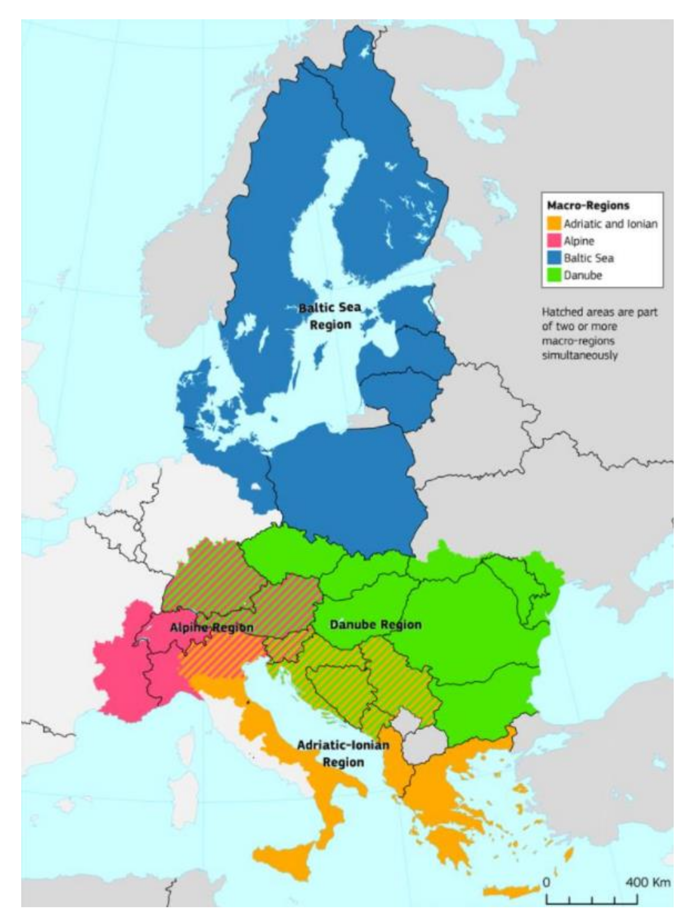
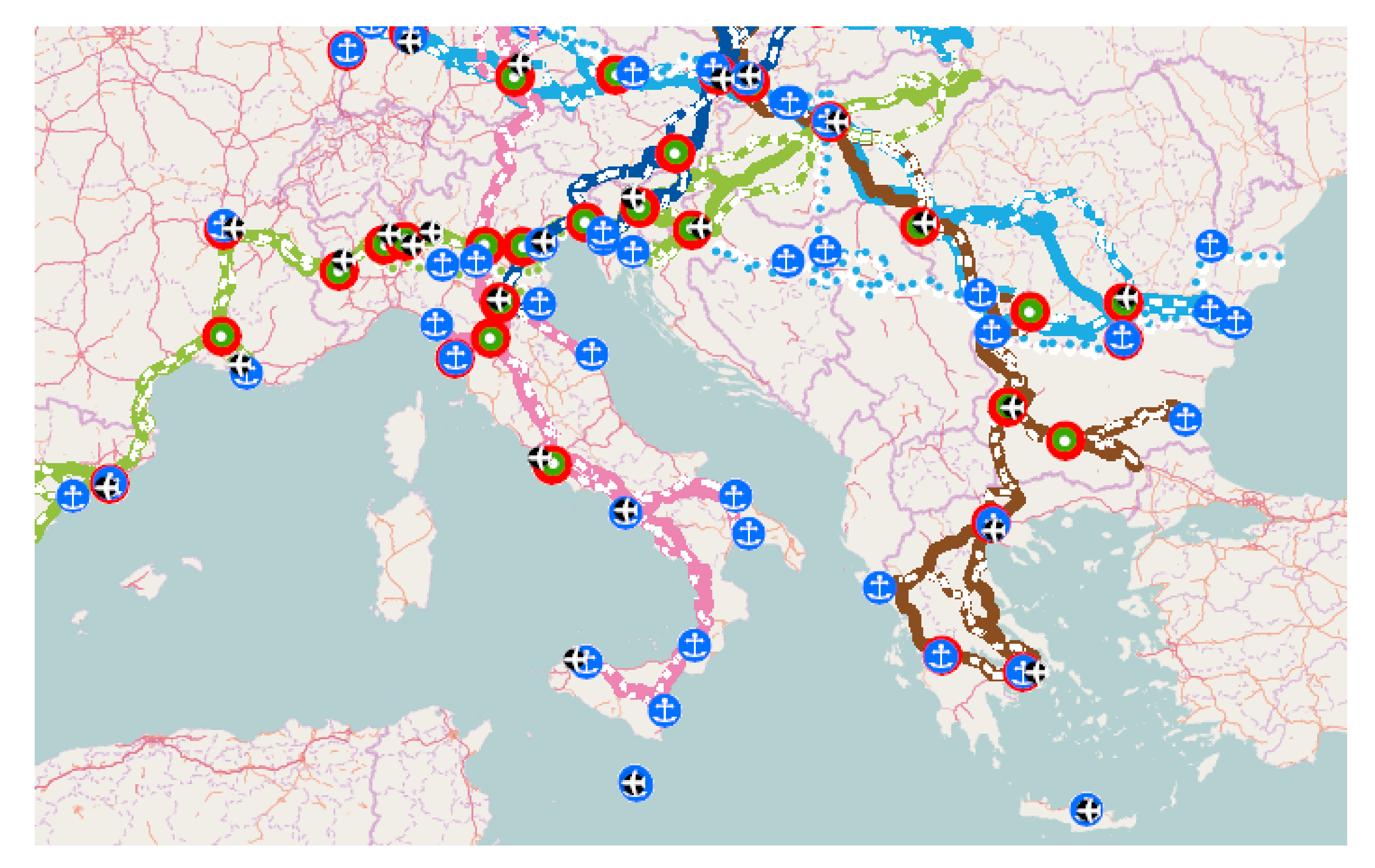
Five of them: Baltic–Adriatic (dark blue), Mediterranean (green), Orient–East Mediterranean (brown), Rhine–Danube (light blue), and Scandinavian–Mediterranean (pink) pass through the Adriatic Ionian Region (
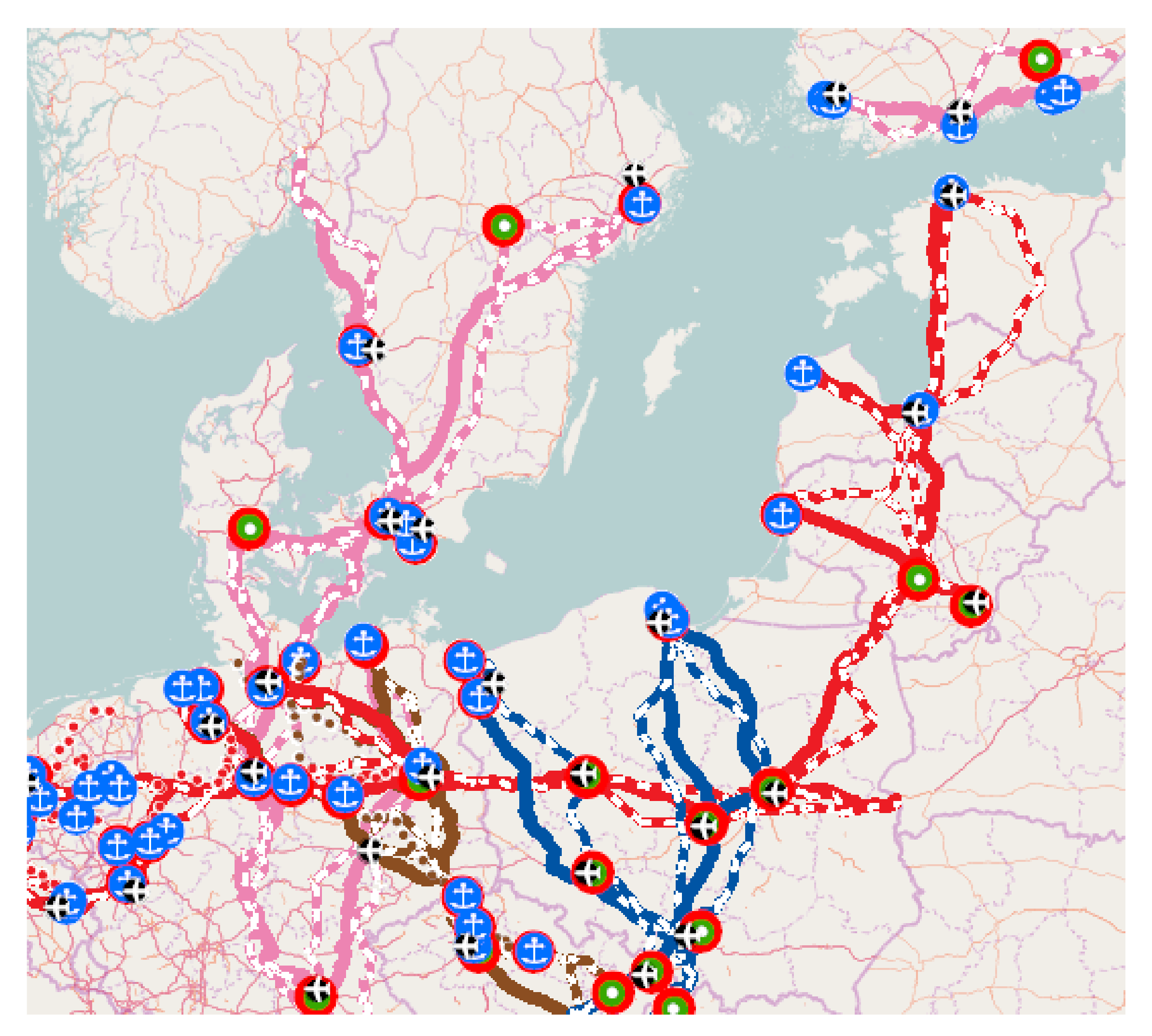
Figure 4). Four of them: Baltic–Adriatic (dark blue), North Sea–Baltic (red), Orient–East Mediterranean (brown), and Scandinavian–Mediterranean (pink) pass through the Baltic Sea Region (
Figure 5).
The Baltic–Adriatic corridor has one of the most crucial road and railway axes in Central Europe. In this corridor, most funds are invested in rail transport. Moreover, in this branch, one can find the highest number of bottlenecks in project implementation. Road transport is the second most-subsidized mode of transport. Poland is mainly funded in this corridor [
53].
The Mediterranean Corridor is the central east–west axis in the TEN-T Network. The corridor is 3000 km long and provides a multimodal link for ports of the Western Mediterranean with the center of the EU. It will let a modal shift from road to rail and connect some of the significant urban areas of the EU with high-speed trains. As in the previous corridor, most funds are also absorbed by rail transport, and this branch has the highest number of bottlenecks. The second branch in the order of subsidies is maritime transport. Among the macro-region countries analyzed, Italy receives the highest subsidy [
54].
The North Sea–Baltic Corridor consists of 5947 km of railways, 4029 km of roads, and 2186 km of inland waterways and connects the ports of the eastern shore of the Baltic Sea with the ports of the North Sea. As in all of the six corridors passing through countries of the two analyzed macro-regions, in this one, rail is also funded chiefly. Similar to the Baltic–Adriatic Corridor, Poland achieved the highest amount of funds. Second, the most-funded branch is road transportation, especially intelligent transportation systems (ITS) [
55].
The Orient–East Mediterranean Corridor connects the roads that pass through European countries in the north–south direction. The Work Plan of this corridor provides the implementation of 649 projects for EUR 89 billion. Rail transport accounts for the vast majority of the CEF fund. It is developed primarily in the southern part of the corridor (mainly Greece). In terms of investment, road transport is in second place. Here, it is worth paying attention to the fact that these are investments in motorways or express roads and alternative fuels (681 charging points are expected to be deployed) [
56].
The Scandinavian–Mediterranean Corridor is interesting from the point of view of this article because it runs through the countries of both macro-regions and, at the same time, is the longest of all the TEN-T corridors. The CEF has granted 91 actions for a total investment worth EUR 6.4 billion. Once again, rail transport infrastructure receives the most funds (around EUR 2 billion). Maritime and road infrastructure will become greener because most actions focus on alternative fuel infrastructure [
57].
The Rhine–Danube Corridor is interesting from the Croatian point of view. It links Central and South-Eastern Europe, but it passes only through Croatia from the macro-regional point. The Work Plan of this corridor includes, among all, a cross-border road bridge constructed between Croatia and Bosnia and Herzegovina on the Sava River. This can be treated as an example of successful cooperation because of the Rhine–Danube Core Network Corridor extension to the neighboring countries [
58].
4.2. The Volume and Structure of Transport in EUSAIR & EUSBSR Countries
In order to summarize and understand investments in the area of transport in the TEN-T corridors, it is worth knowing the size and structure of transport in the countries of the macro-regions described. Rail transport will be analyzed first. Its importance in the development strategy of the macro-regions is exceptionally high. In the Work Plans of the individual TEN-T corridors, investments in rail transport are by far the largest. The question then arises: does the infrastructure and volume of rail transport in individual countries allow for the full use of this mode of transport? Firstly, in terms of infrastructure, rail transport is more developed in the Baltic Sea Region (EUSBSR). It is already visible in the analysis of the total length of railway lines in 2019 (
Figure 6).
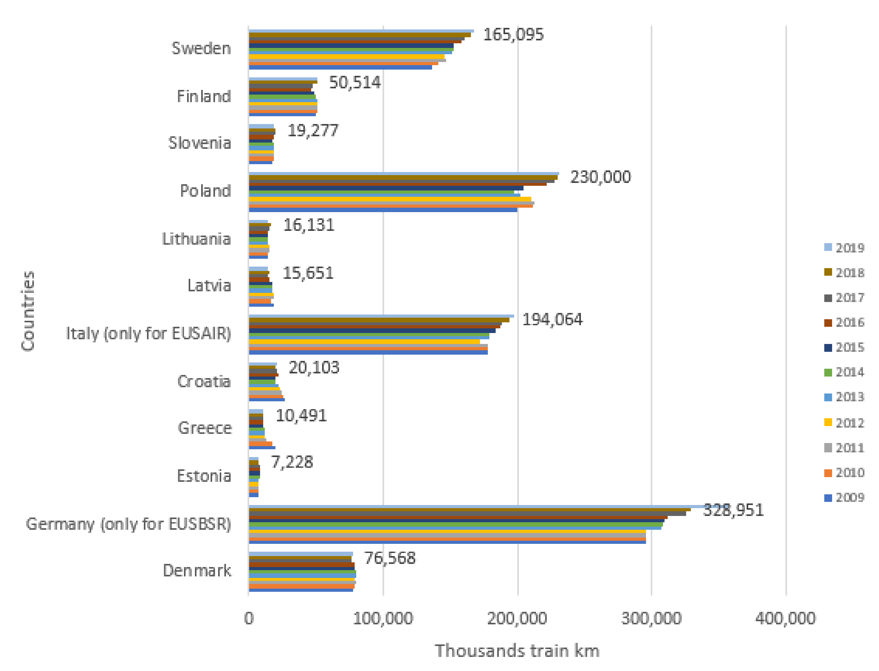
Secondly, the railway traffic is interesting, expressed by thousands of train kilometers. In the EUSBSR in 2019, this traffic was over three times higher than in EUSAIR. At the same time, even though Italy has a progressive movement individually, Germany is in the lead in the Baltic Sea Region, followed by Poland and then Sweden (
Figure 7).
The expenditures and individual investments of each country in railway infrastructure and rolling stock are also interesting. Although not all countries provide complete statistical information, the Baltic countries invest much more internal funds in rail transport than countries from the EUSAIR region. In case of investments in rolling stock, Poland invests the most prominent funds. It is a natural phenomenon related to the general development of rail transport in this country and rather the replacement of the several decades-old rolling stock with a new one and the implementation of high-speed railways, including the Pendolino. In turn, the largest expenditure on infrastructure was made in Sweden.
The situation is interesting in the case of maritime transport. Here, the assumptions of the EUSAIR Action Plan aimed at developing this particular mode of transport are not surprising. Maritime transport in both regions is characterized by handling of goods. Ultimately, the volume of the entire shipment in both macro-regions is comparable, and, in 2019, it accounted for 14.8% in the EUSBSR and 13.2% in the EUSAIR of all maritime transport in the EU countries (
Figure 8).
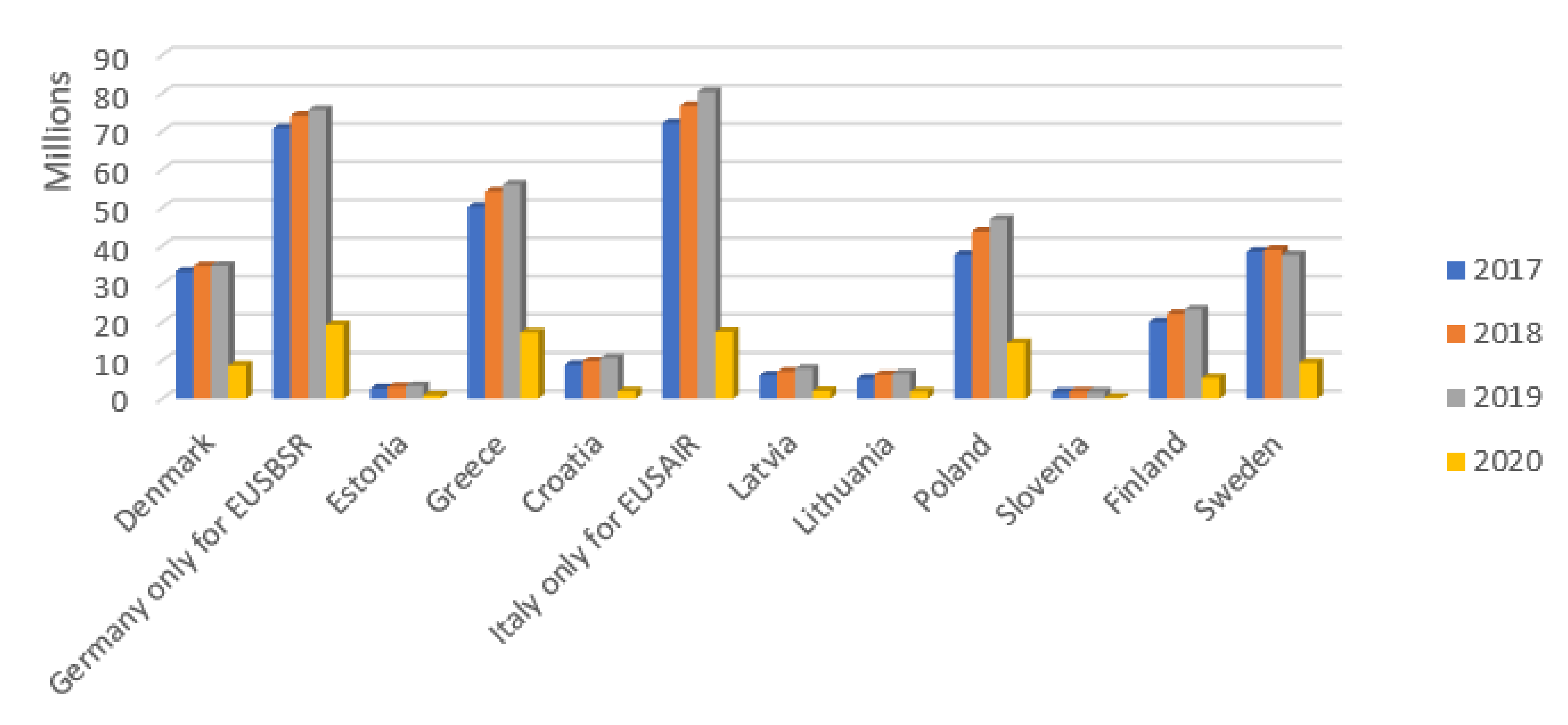
As far as air transport is concerned, it should be emphasized that, despite the increase in gas emissions from this mode of transport in general, it still emits less of these gases together with maritime transport than the entire road transport. In the last decade, air transport recorded a significant increase in passengers handled. This was visible in Central Europe. For example, in Poland in 2011, more than 20 million passengers were handled, while, in 2019, there were more than twice as many, almost 47 million. The COVID-19 pandemic saw a dramatic drop to 14.5 million in 2020. The summary of the number of passengers handled in the countries of the macro-regions between 2017 and 2020 is presented in
Figure 9.
Although Italy (even only for the EUSAIR region) is the leader in the carriage of passengers by air compared to other countries in 2019, the EUSBSR region countries carried more passengers in total. Germany was ranked second, followed by Greece. In total, however, as can be seen in
Figure 10, passenger transport in the EUSBSR accounted for 21% of the total air transport in the EU, while, in the EUSAIR, it accounted for 13%.
As for the infrastructure base, it is larger in the EUSBSR countries (
Figure 11). However, this should be linked to the number of countries in this macro-region (8). In the EUSAIR region, the infrastructure is even more developed, but it is smaller due to the smaller number of countries (4) in total. Again, it is worth referring to the macro-region development strategy. In the EUSAIR, particular attention is paid to maritime transport. So far, however, due to the tourist nature of many areas of Italy or Greece, air transport has been the most preferred method of international transport.
Taking into account climate issues, mainly the fact that the level of gas emissions in maritime and aviation transport is similar (approximately 13% each), it is worth considering whether, instead of new investments in maritime infrastructure, it is better to use the current one, the existing aviation infrastructure, also in the field of freight transport and connecting the region in general.
As for road transport, to illustrate its size, in
Figure 12, a comparison of the transport of goods (in thousands of tons) by various modes of transport in the countries of the macro-regions in 2019 is presented.
The last year before the coronavirus pandemic showed that the share of road transport in transporting goods was the highest in most macro-region countries. The exception was Estonia, where more goods were transported by sea. Some kind of diversification of transport can also be noticed in Latvia and Lithuania. However, road transport plays a key role. Of course, one can analyze the resources of road infrastructure, but, in light of the assumptions of the macro-region development strategies (EUSBSR & EUSAIR), it is necessary to consider which mode of transport in a given country and to what extent can replace the road one. For example, despite the well-developed infrastructure, the insignificant share of air transport is a wonder. Particularly noteworthy is rail transport, which has incurred enormous expenditure in recent years.
Moreover, the European Commission has declared 2021 the European Year of Rail as part of the EU’s efforts under the European Green Deal to achieve climate neutrality by 2050. In these modes of transport, there are also interesting cases of an increase in the share of the transport of goods during the pandemic (in 2020); i.e., Croatia recorded an increase in the transport of goods by rail in 2020 compared to previous years. In turn, Lithuania recorded such an increase in air transport.
4.3. Allocation of the CEF Funds
The Connecting Europe Facility (CEF) Regulation, adopted in 2013, allocated a seven-year budget (2014–2020) of EUR 30.4 billion, of which EUR 24 billion are for the transport sector [
51]. On 2 May 2018, the Commission proposed a new long-term budget for the period of 2021 to 2027, where the focus remains on developing the Trans-European Network, with a particular priority on cross-border sections and missing links of the TEN-T Core Network. The allocation of CEF funds is a kind of exemplification of the actual needs and the direction of transport development. The division of the fund can be presented through the prism of the top five priority areas of planned investments and by type of transport. Below, in
Table 5 and
Table 6, the allocation of the fund (in millions of Euros) to the countries of the EUSBSR macro-region is shown. The lack of data in some table columns means that the budget was meager or no data were made available.
The largest allocation of CEF funds in the 2014–2020 financial perspective for the EUSBSR was recorded for the European Rail Traffic Management System. It is worth noting that almost 59% of these funds have been invested in Poland. The SESAR program turned out to be the second priority of CEF in terms of the amount of invested funds, with over 67% of them invested in Germany. Moreover, Poland’s participation in investments in the Intelligent Transport Services for road (ITS) program attracts attention. The analyzed financial perspective amounted to almost 98% of all funds spent on this priority.
The 2014 to 2020 CEF financial perspective for the EUSBSR can be characterized as a period of making high investments in rail transport with the share of almost 80% of CEF funds spent on all modes of transport. Considering over eight times greater expenditure on rail transport than on road transport and the aforementioned dominance of road transport in the context of the tonnage of transported goods, it requires reflection over the level of effectiveness of the implemented investments. Less than a 5% share of expenses on maritime transport also makes one think about the compliance of practical activities with the assumptions formulated in the EU Strategy for the Baltic Sea Region. Below, in
Table 7 and
Table 8, the allocation of the fund (in millions of Euros) to the countries of the EUSAIR macro-region is shown. As before, the amount of investment for five priority CEF programs and individual modes of transport has been presented in two separate tables.
The largest allocation of CEF funds in the 2014 to 2020 financial perspective for the EUSAIR was recorded for the Single European Sky-SESAR program. It is worth noting that almost 75% of these funds have been invested in Italy. ERTMS was next in terms of the size of investments. In this case, again, the most considerable amount of money was spent in Italy.
As in the case of the EUSBSR, also in the case of the EUSAIR, the analyzed financial perspective for 2014 to 2020 can be described as the period of major investments in rail transport. The issue of low expenses on maritime transport seems interesting again.
4.5. Panel Data Model of Greenhouse Gas Emissions
Econometric analysis aimed to assess the significance and influence direction of the volume of freight transport (broken down by means of transport on the amount of air pollution with greenhouse gases. To compare EUSAIR to EUSBSR area in terms of transport impact on greenhouse gas emissions, two panel data models (N
EUSAIR = 4, N
EUSBSR = 8, T = 2005–2019) were constructed and estimated. A panel data regression differs from a regular time-series or cross-section regression in that it has a double subscript on its variables (2)
where
i denotes the cross-section dimension, whereas
t denotes the time-series [
59] dimension,
yit is a dependent variable,
α is a scalar (constant term),
β is K × 1, and
xit is the
i-th observation on K explanatory variables;
denotes the error term.
From the point of view of econometric modeling, the most important feature is the possibility of avoiding bias of the estimator due to the omission of an important explanatory variable. It can lead to false, contradictory results. Models for panel data make it possible to estimate the individual effects of the factors impact (2), contributing to the differentiation of the observed units not included in the model, constant over time and/or (3) time effects, unchanged for all units, characteristic for individual years. There are two basic methods taking into account individual effects (individual or time). The
fixed effect model (FEM) formulation assumes that differences across units (individuals or time) can be captured in the constant term. The fixed effect model takes
(3) to be an unobservable, individual (or time)-specific constant term in the regression model [
60].
The
random effect model (REM) approach specifies that
(4) is a group specific random element. The random effects model is appropriate for choosing N individuals randomly from a large population. In this case, N is usually large, and a fixed effects model would lead to an enormous loss of degrees of freedom.
where
denotes the unobservable individual (time)-specific effect and νit denotes the remainder disturbance.
Note that is time-invariant (or is individuals-invariant) and it accounts for any individual-specific effect (or time-specific effect) that is not included in the regression.
The following issue is estimating the indicated permanent effects (individual or time). The first model with intragroup effects, the so-called
within model, uses deviations of a variable’s value from the group (individuals or time) average. The model is estimated without a constant using the Ordinary Last Squares (OLS). Estimated coefficients measure the effect of changes in the explanatory variable on the value of the dependent variable. The model does not take into account changes between groups. The second,
between model, is computed on time (or individual) averages of the data, discards all the information due to intragroup variability but is consistent in some settings (e.g., nonstationarity) where the others are not, and is often preferred to estimate long-run relationships [
59].
To choose the most appropriate estimator, the parameters and error terms hypotheses are tested using: (I) Testing for fixed effects (F-test). The null hypothesis is the same constant term applied across all individuals; (II) if the homogeneity assumption over the coefficients is established, the next step is to establish the presence of unobserved effects, comparing the null of spherical residuals with the alternative of individuals (or time units) specific effects in the error term (Breusch–Pagan test). (III) The choice between fixed and random effects specifications is based on Hausman test, comparing the two estimators under the null of no significant difference: if it is not rejected, the more efficient random effects estimator is chosen. In order to select the optimal model for inference, several models were estimated, taking into account the combinations of the above-mentioned methodological assumptions. The selection was then made based on the indicated statistical tests.
The first stage of constructing the theoretical form was selecting the functional form and indication of the dependent and explanatory variable. The dependent variable was assumed total national greenhouse gas emissions (from both ESD and ETS sectors) in tons per capita. This indicator included the so-called ‘Kyoto basket’ of greenhouse gases, that is, carbon dioxide (CO
2), methane (CH
4), nitrous oxide (N
2O), and the so-called F-gases) from all sectors of the GHG emission inventories (including international aviation and indirect CO
2) [
61]. The explanatory variables were defined as the volumes of goods transported by road [
62], rail [
63], maritime [
64], and air [
65] transport in thousand tons. In order to take into account the economic importance of the transport modes, the volume of transported goods of each of them was divided by the GDP value of individual countries [
66] (in Purchasing Power Standards, for EU-27, constant prices 2005 [
67]). The power function was chosen as the functional form of the model. Estimates of explanatory variables parameters indicate the flexibility of changing the emission volume per capita to the change in the volume of loaded goods to GDP. After transforming the model equation into a linear form concerning the parameters (condition for the OLS estimator use), the theoretical model assumed the logarithmic form (5)
where:
denotes constant term,
, …, —estimated parameters,
—error term,
—total national greenhouse gas emissions in tons per capita in i-th country and t-th year;
—volumes of goods transported by road in thousand tons in terms of GDP i-th country and t-th year;
—volumes of goods transported by railway transport in thousand tons in terms of GDP i-th country and t-th year;
—gross weight of goods handled in all ports in thousand tons in terms of GDP i-th country and t-th year;
—volumes of freight and mail air transport in thousand tons in terms of GDP i-th country and t-th year.
One of the terms for using OLS is the lack of correlation between the explanatory variables. In order to verify this assumption, the Pearson linear correlation coefficients for the model variables were calculated (
Table 10). It is necessary to point out a high relationship between the volume of cargo transported by rail and maritime transport (0.906). Despite the high correlation, it was decided to include the variable in the models. It is worth noting the occurrence of differences between EUSAIR and EUSBSR in the correlation of pollution and the tonnage of transported loads. In the group of EUSAIR countries, an increase in the tonnage of cargo transported by rail contributed only to reducing pollution. In the case of the EUSBSR countries, all types of transport, except air transport, showed such a relationship. Moreover, the correlations between the sizes of loads broken down by modes of transport indicate complementarity (maritime transport with road transport) and substitutability (air transport vs. road and railway transports).
The next stage of the analysis was to estimate five variants panel data model: Pool (OLS), FEM (within-time), FEM (within-individual), FEM (between-time), REM (time). Before interpreting the results, the model with the best statistical properties was selected based on the tests (F-test, Breusch–Pagan test, Hausman test) (
Table 11). The estimation results are presented in
Table 12 and
Table 13. Due to the comparability of the model estimation methods for the EUSAIR and EUSBSR, and high level of matching the models to empirical data (Adjusted R
2), the Fixed Effect between the model for time units (FEM between-time) was selected. Interpretation of individual parameter estimation took into account the ceteris paribus assumption.
The FEM (between-time) model estimation results (
Table 12 and
Table 13) show the following conclusions. Among the countries of both areas (EUSAIR, EUSBSR), the estimates showed a statistically significant (
p < 0.05) positive impact on the volume of loads transported by road transport. An increase in volume loads by 1% resulted in an increase in air pollution by 0.446% (EUSAIR) and 0.728% (EUSBSR). In reference to loads’ road transport changes, the elasticity of air pollution was the highest compared to other modes of transport in the studied areas. This proves the highest emissivity of road transport.


 ,
, 


