Spatial Spillover Effect of Carbon Emissions and Its Influencing Factors in the Yellow River Basin

Abstract

The high-quality development of the Yellow River Basin is the focus of China’s development. A spatial lag model and a spatial error model were constructed. The mechanism of spatial spillover effects of economic growth, industrial structure, urbanization level on carbon emissions of all provinces in the Yellow River Basin were analyzed. The results show that: (1) There are obvious spatial spillover effects and spatial agglomeration characteristics of provincial carbon emissions. The carbon emissions of Shandong, Shanxi, Shaanxi, Henan, Inner Mongolia, Sichuan show a high–high agglomeration feature, while the carbon emissions of Gansu, Qinghai and Ningxia show a low–low agglomeration feature. (2) The relationship between carbon emissions and economic growth in the whole Yellow River Basin shows a “U” shaped EKC curve, while the relationship between carbon emissions and economic growth in the Yangtze River Basin shows an inverted “U” shaped EKC curve, and the two aspects are in stark contrast. The population size, industrial structure and urbanization level can promote carbon emissions, while technology plays a role in curbing carbon emissions in the Yellow River Basin. The measures to reduce carbon emissions should be achieved in terms of regional joint prevention and control, transformation of economic growth, optimization of industrial structure, and strict implementation of differentiated emission reduction policies.

1. Introduction

Ecological protection and high-quality development of the Yellow River Basin have become one of China’s major national strategies. The Yellow River basin is the “China’s mother” river and the second longest river after the Yangtze River Basin in China. The Yellow River originates from the Bayankala Mountains in Qinghai, and flows through nine provinces and regions in Qinghai, Sichuan, Gansu, Ningxia, Inner Mongolia, Shaanxi, Shanxi, Henan and Shandong, and finally empties into the Bohai Sea at Kenli County, Dongying City, Shandong Province. Standing at the strategic height of the great rejuvenation of the Chinese nation, General Secretary Xi Jinping personally outlined a major national strategy for ecological protection and high-quality development of the Yellow River Basin.

On 18 September 2019, General Secretary Xi Jinping presided over a symposium on Ecological Protection and High-quality Development of the Yellow River Basin, pointing out the direction of ecological protection and high-quality development of the Yellow River basin. As the Yellow River basin is an important energy and chemical raw materials and basic industrial base in China, the environmental protection needs to be improved and perfected. In recent years, the basin has accounted for more than a third of the country’s carbon emissions. Under the vision of carbon peak and carbon neutralization, it is of strategic significance to study the current situation, influencing factors and spatial spillover effects of carbon emissions in the Yellow River Basin for promoting the green and low-carbon development of the Yellow River Basin and promoting the coordinated emission reduction of the whole basin.

Based on STIRPAT’s traditional model, this paper expands to explore the impact of different economic and social factors on carbon emissions. Specifically, this paper will discuss the following issues: (1) Incorporating the spatial effect in the process of influencing carbon emissions, considering the dependence of spatial units and the spatial effect of economic activities, exploring the mechanism of spatial correlation of carbon emissions, and using spatial panel model to analyze the influence of various factors on carbon emissions. (2) Based on EKC theory, the interaction between economic growth and carbon emissions is analyzed to accurately grasp regional development stages and formulate corresponding emission reduction policies. (3) Using the same way to analyze the mechanism of economic and social factors and carbon emissions in the Yangtze River Basin. Furthermore, the carbon emissions of the Yellow River basin and the Yangtze River basin are compared and analyzed to provide reference for the future low-carbon development of the Yellow River Basin.

The research methods and conclusions about the driving factors of carbon emissions are multi-layered. Most of the research methods focus on structural decomposition, “IPAT” model, STIRPAT model, Granger causality test, and so on [1,2,3]. Most of the methods analyze the influencing factors of carbon emissions from the perspectives of energy intensity, industrial structure, residents’ income improvement and adjustment of openness [4,5]. Among them, economic growth is the main factor promoting carbon emissions. The conclusion drawn under this research background often leads people to misunderstand that the increase in regional carbon emissions is the result of local economic growth. Hu Yi (2019) pointed out that trade activities shift the place of production and the place of final consumption of goods and change the spatial and temporal distribution characteristics of carbon emissions [6]. At the same time, carbon dioxide itself has a certain diffusion effect. Therefore, there may be many reasons for the increase of carbon emissions in a certain region, among which the spillover effect of trade activities and carbon dioxide itself is a major focus that cannot be ignored.

In addition, studies on the relationship between economic growth and carbon emissions are generally conducted by means of panel data analysis and time series analysis. Li et al. (2020) used time series data to analyze the long-term trend and short-term change characteristics between carbon emissions and economic growth [7]. Arshed et al. (2021) analyzed that the EKC curves between economic growth and carbon emissions in different regions have different shapes by using panel data of Provinces in China [8]. However, there are some defects in analyzing the relationship between carbon emissions and economic growth whether using panel data or time series data. Time series cannot analyze the heterogeneity of carbon emissions in different regions, while panel data lacks the spatial effect analysis of each variable.

Based on the above problems, some scholars have included spatial effect in relevant studies. The extended STIRPAT model by Sun et al. (2021) assessed the impact of various factors on CO₂ emissions in different cities in the Yellow River basin [9]. Burnett et al. (2013) analyzed the relationship between carbon emission and economic growth by using spatial panel model [10]. Li et al. (2020) used spatial panel data to analyze the impact of China’s provincial energy investment and economic development on carbon emission reduction [11]. Chen et al. (2020) explored the influencing factors and spatial spillover effects of agriculture by estimating the spatial panel data model of 31 provinces in China and found that the growth of per capita GDP was the main driving force to accelerate the growth of agricultural carbon emissions [12]. Wang et al. (2015) and Xue et al. (2021) studied the factors influencing the spatial effect of carbon dioxide in Energy-intensive industries in China [13,14]. Wu et al. (2021) analyzed the spatial and temporal distribution characteristics of land use and carbon emissions in China from 1997 to 2016 and found that income, population, energy intensity, energy structure and economic structure can help explain the change of industrial land space emissions [15]. Yang et al. (2021) analyzed the impact of technological factors in various sectors on carbon emissions in China from a spatial perspective [16]. Some scholars also analyzed the carbon emission intensity and spatial correlation at the provincial level in China from the aspects of technological progress, structure adjustment and industrial structure adjustment [17,18,19]. Miao et al. (2020) analyzed the upgrading effect of industrial collaborative agglomeration and carbon emissions [20].

To sum up, spatial panel data can be more reasonably and effectively applied to the research of carbon emissions. At present, most of the research on the Yellow River basin focuses on water resources management and protection, while the research on air pollution and carbon emission is still in its infancy. Therefore, the innovation of this paper lies in the use of spatial econometrics to analyze the impact of different economic and social factors on carbon emissions, such as population size, technological development level, economic growth, industrial structure and urbanization level. The spatial effects of carbon emissions in nine provinces of the Yellow River Basin were analyzed by using different weight matrices. The contribution of this paper is to comprehensively explore the influencing factors and spatial effects of carbon emissions in the Yellow River basin by using spatial econometric model combined with the regional characteristics of the Yellow River Basin and provide theoretical support and data reference for the future high-quality development of the Yellow River Basin.

2. Materials and Methods

2.1. Model Setting

Among the many research methods of carbon emission influencing factors, the STIRPAT model constructed by Dietz and Rosa is widely used (York, 2003) [2]. The general form of the STIRPAT model is as follows:

$$I=a{P}^b{A}^c{T}^d\mu$$

(1)

Among them, $I$ is human impact, which represent environmental pressure. P represents population. A is per capita GDP, which represents economic level. T is technology, which represents technical level. a, b, c, d are parameters to be estimated, $\mu$ is a random error.

The STIRPAT model has better flexibility and can be expanded appropriately. The expandable characteristics of the model will be used to investigate the spatial spillover effects of neighboring provinces on the province. The spatial characteristics caused by economic level and industrial structure (IS) will be explored. The logarithmic form of the extended model is as follows:

$$\begin{array}{c}\ln I=\ln \alpha +{\beta }_1\ln pGD{P}_{it}+{\beta }_2{(\ln pGD{P}_{it})}^2\\ \hspace{1em}\hspace{1em}\hspace{1em}\hspace{1em}+{\beta }_3\ln I{S}_{it}+{\beta }_4\ln P_{it}+{\beta }_5\ln T_{it}+{\beta }_6\ln U_{it}+\epsilon \end{array}$$

(2)

where $I$ is carbon emissions, $pGDP$ means per capita gross regional product. IS represents the proportion of the secondary industry’s GDP to the total GDP. P is the population. U is the level of urbanization. and T represents energy intensity. $\epsilon$ is a random disturbance item.

The analytical framework and model setting of this spatial econometric model (Sun et al., 2014) were adopted [21]. Based on Equation (2), the spatial lag panel model (SLM) and the spatial error model (SEM) are established and as follows:

$$\begin{array}{c}\ln I_{it}=\rho {\displaystyle \sum _{j=1}^n{w}_{ij}}\ln I_{jt}+{\beta }_1\ln pGD{P}_{it}+{\beta }_2{(\ln pGD{P}_{it})}^2\\ \hspace{1em}\hspace{1em}\hspace{1em}\hspace{1em}\hspace{1em}\hspace{1em}+{\beta }_3\ln I{S}_{it}+{\beta }_4\ln P_{it}+{\beta }_5\ln T_{it}+{\beta }_6\ln U_{it}+{\mu }_i+{\lambda }_t+{\epsilon }_{it}\end{array}$$

(3)

$$\begin{array}{c}\ln I_{it}={\beta }_1\ln pGD{P}_{it}+{\beta }_2{(\ln pGD{P}_{it})}^2+{\beta }_3\ln I{S}_{it}+\\ \hspace{1em}\hspace{1em}\hspace{1em}\hspace{1em}{\beta }_4\ln P_{it}+{\beta }_5\ln T_{it}+{\beta }_6\ln U_{it}+{\mu }_i+{\lambda }_t+{\phi }_{it}{\phi }_{it}\\ \hspace{1em}\hspace{1em} =\delta {\displaystyle \sum _{j=1}^n{w}_{ij}}{\phi }_{jt}+{\epsilon }_{it}\end{array}$$

(4)

where $i$ is different provinces, $n$ is the number of provinces, $t$ is different years. Both $\rho$ and $\delta$ represent the spatial autoregressive coefficient, $w_{ij}$ represents the element in the spatial weight matrix $W$, ${\phi }_{it}$ is the random error term, ${\mu }_i$ represents the individual fixed effect, ${\lambda }_t$ represents the time fixed effect, ${\epsilon }_{it}$ is the random disturbance term, and ${\epsilon }_{it}~i.i.d(0,{\sigma }^2)$.

2.2. Data Processing

2.2.1. Data Sources

Panel data of nine provinces in the Yellow River Basin from 2000 to 2018 were selected as research samples. The economic and social data involved in this paper come from China’s Regional Economic Statistical Yearbook, China’s Energy Statistical Year book and the statistical yearbook of each province’s statistics bureau over the years. The longitude and latitude information of different regions is collected by Baidu map.

2.2.2. Variable Description

• Explained variable. Provincial level estimation is mainly achieved by using the balance algorithm based on fossil energy consumption [22]. The carbon emissions here refer to the carbon emissions from primary energy consumption. And the carbon emission coefficient method is used to calculate the carbon emissions:

  $$I={\displaystyle {\sum }_{i=1}^n{E}_i\cdot F_i}$$

  (5)
  Among them, $I$ represents carbon emissions, E_i represents the i-th energy consumption, and F_i represents the i-type energy carbon emission coefficient. This paper mainly calculates the consumption of three fossil energy sources: coal, oil, and natural gas. The carbon emission coefficients of coal, oil and natural gas are 0.7476 kg carbon/kg standard coal, 0.5825 kg carbon/kg standard coal, and 0.4435 kg carbon/kg standard coal, which use the values recommended by the National Development and Reform Commission.
• Explanatory variables. In terms of economic growth, the quadratic term of per capita GDP is incorporated into the model to analyze the embodiment of environmental Kuznets curve theory in the sample period. Industrial structure (IS) is measured by the proportion of the secondary industry in the total output value. Compared with the primary and tertiary industries, the secondary industry is more dependent on fossil energy and can bring more greenhouse gas emissions. Technological level (T) is represented by energy intensity. With the rapid development of economy, technological progress has multiple impacts on the environment, including both positive and negative impacts. The larger the population (P), the greater the demand for energy, and more pollutants will be generated, which will bring some pressure to the environment.

The urbanization level (U) is represented by the proportion of urban population in the total population. Many scholars believe that the development of urbanization level will have different degrees of impact on carbon emissions. In order to eliminate the effect of heteroscedasticity, logarithmic analysis is performed on all variables. Meanings and units of all relevant variables as shown in

Table 1. Meaning and units of related variables.

Variable	Meanin	Unit
I	Carbon emissions	ten thousand tons
P	Population	ten thousand tons
PGDP	per capita GDP	ten thousand yuan/ten thousand people
T	Energy strength	ten thousand tons of standard coal/ten thousand people
IS	Industrial structure	%
U	Urbanization level	%

.

2.2.3. Spatial Weight Matrix of Carbon Emissions

This paper uses geographic weight matrix and economic–geographic weight matrix to analyze the spatial spillover effects of carbon emissions (Zhao et al., 2020) [23].

• Geographic weight matrix. The geographic weight matrix adopts a spatial adjacency matrix, and the carbon dioxide emissions of provinces adjacent to each other will inevitably affect each other. If the matrix element is expressed as: area $i$ and area $j$ are adjacent, then $w_{ij}=1$, if not adjacent, it is 0, and the main diagonal element $w_{ij}=0$ indicates that the distance between the local area and the local interval is 0. The matrix form is $W=(w_{ij}{)}_{n\times n}$, where $n$ is the number of provinces (Liu, 2015) [24]. At the same time, the weight matrix needs to be standardized so that the sum of the row elements is 1. As shown in Equation (6):

  $$W_1=\left(\begin{array}{ccc}{w}_{11}& \dots & w_{1n}\\ ⋮& \ddots & ⋮\\ w_{n1}& \cdots & w_{nn}\end{array}\right)$$

  (6)

  The element representation is as follows:

  $${\mathrm{W}}_{ij}=\{\begin{array}{c}1, \mathrm{Space} \mathrm{unit} i \mathrm{and} \mathrm{space} \mathrm{unit} j \mathrm{are} \mathrm{adjacent} \\ 0, \mathrm{Space} \mathrm{unit} I \mathrm{and} \mathrm{space} \mathrm{unit} J \mathrm{are} \mathrm{not} \mathrm{adjacent} \end{array}$$

  (7)
• Economic–geographic weight matrix. It is relatively rough to reflect the spatial relationship of regions only by geographic location characteristics (Li, 2010) [25]. Regional development is an integral activity. The impact of this activity process is not only from the regions close to the geographical distance, and it is multi-faceted and multi-level. Therefore, in order to comprehensively consider various spatial influencing factors, this paper nests socioeconomic characteristics and geographic location characteristics to construct a weight matrix. As shown in Equation (8):

  $$W_2=W_1\mathrm{dia}g({\overline{X}}_1/\overline{X},{\overline{X}}_2/\overline{X},\cdots ,{\overline{X}}_n/\overline{X})$$

  (8)

  where $W_1$ is the geographical weight matrix. ${\overline{X}}_i=1/(t_1-t_0+1){\displaystyle {\sum }_{t_0}^{t_1}{X}_{it}}$ is the average value of the total output value of province $i$ during the investigation period, $\overline{X}=\frac{1}{n(t_1-t_0+1)}{\displaystyle \sum _{i=1}^n{\displaystyle {\sum }_{t_0}^{t_1}{X}_{it}}}$ is the average value of the total output value of all regions during the investigation period, and $t$ is the different period.

3. Empirical Analysis

3.1. Spatial Correlation Test

3.1.1. Global Spatial Autocorrelation Test

In order to make a more accurate explanation of the spatial spillover effect of carbon emissions, and to test whether there is global correlation of carbon emissions among provinces. The calculation formula of the global Moran’s I is as follows:

$${Moran}^{\prime }sI=\frac{{\displaystyle {\sum }_i{\displaystyle {\sum }_j(Y_i-\overline{Y})(Y_j-\overline{Y})}}}{S^2{\displaystyle {\sum }_i{\displaystyle {\sum }_j{w}_{\begin{array}{l}ij\\ \end{array}}}}}$$

(9)

$$S^2=\frac{1}{n}{\displaystyle \sum _i(Y_i}-\overline{Y})$$

(10)

$$Y=\frac{1}{n}{\displaystyle \sum _i{Y}_i}$$

(11)

In the formula, $Y_i$ and $Y_j$ are the observed values, and $w_{ij}$ is the elements of the weight matrix. The value of Moran’s I is generally between −1 and 1. More than 0 indicates positive autocorrelation, that is, the high value is adjacent to the high value, and the low value is adjacent to the low value. Less than 0 is negative autocorrelation, that is, the high value is adjacent to the low value. Close to 0, it means that there is no spatial autocorrelation. The global Moran’s I is used to measure the spatial agglomeration effect of a certain variable in the overall area.

The geographic weight matrix and the economic–geographic weight matrix are used to calculate the global Moran’s I from 2000 to 2018 in

Table 2. Moran’s I of carbon emissions from the Yellow River Basin from 2000 to 2018.

Years	Geographic Weight Matrix		Economic–Geographic Weight Matrix
	Moran’s I	p-Value	Moran’s I	p-Value
2000	0.023	0.216	0.039	0.028
2001	0.028	0.023	0.034	0.046
2002	0.156	0.040	0.169	0.060
2003	0.227	0.021	0.226	0.002
2004	0.238	0.043	0.295	0.005
2005	0.322	0.091	0.341	0.009
2006	0.326	0.096	0.343	0.004
2007	0.326	0.008	0.328	0.008
2008	0.335	0.069	0.349	0.002
2009	0.327	0.093	0.341	0.009
2010	0.325	0.009	0.336	0.007
2011	0.332	0.037	0.332	0.007
2012	0.328	0.029	0.323	0.207
2013	0.340	0.004	0.345	0.000
2014	0.336	0.005	0.342	0.000
2015	0.352	0.005	0.355	0.006
2016	0.369	0.006	0.360	0.001
2017	0.367	0.008	0.375	0.004
2018	0.389	0.007	0.453	0.040

. From an overall point of view, Moran’s I are all positive. The proximity of provinces or the close relationship between economic and geographic activities have a positive spatial autocorrelation for their carbon emissions. The relevance also further illustrates that the carbon emissions of the provinces in the Yellow River Basin affect each other. Table 1 shows that Moran’s I under different weights are different, and the value of Moran’s I under the economic–geographic weight matrix and its significance are significantly better than the geographic weight matrix. The Moran’s I values obtained under the geographic weight matrix and the economic–geographic weight matrix increased year by year. Notably, the Moran’s I value in 2018 under the economic–geographic weight matrix reached 0.453, which shown a strong positive spatial correlation. It is significant at the 5% level.

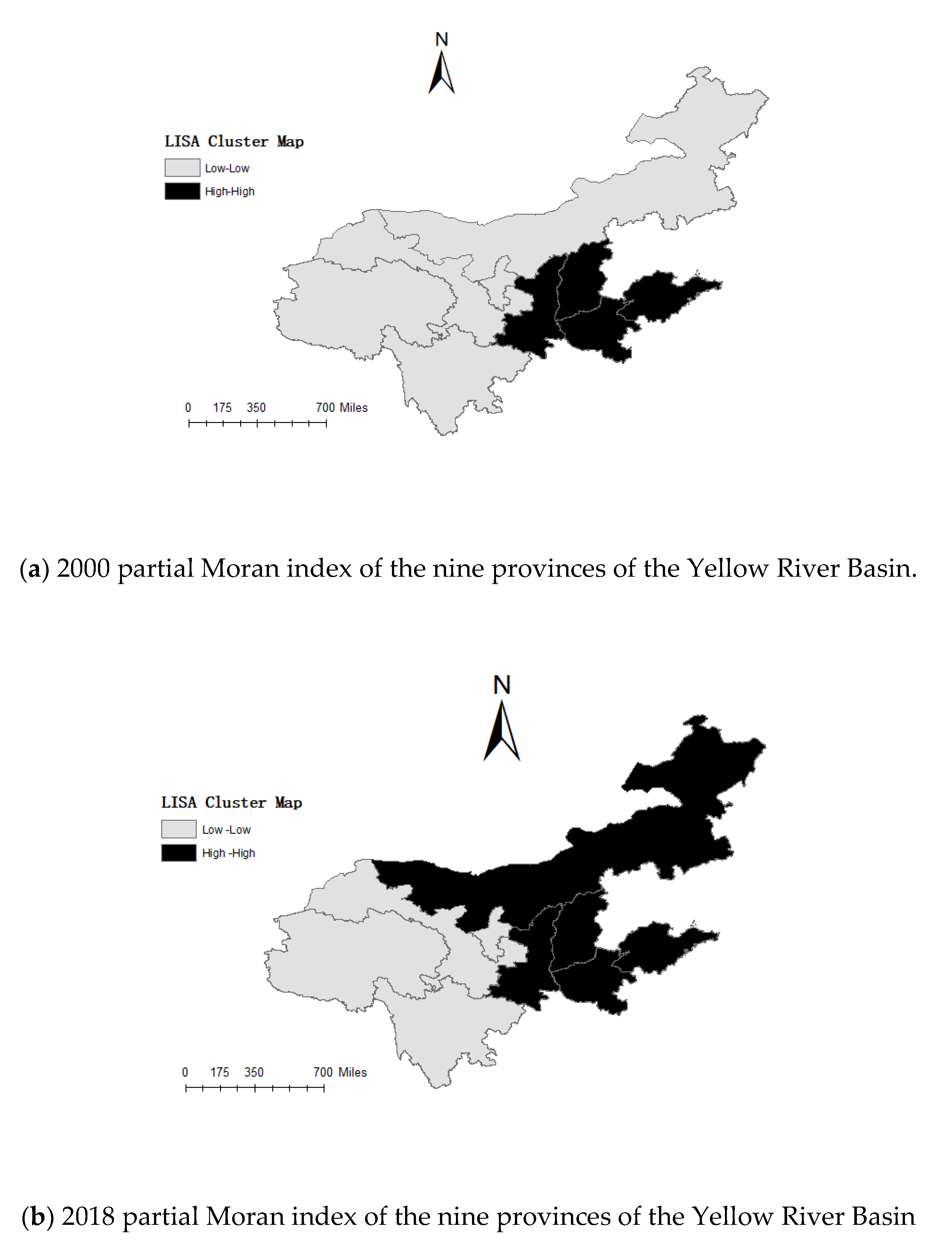
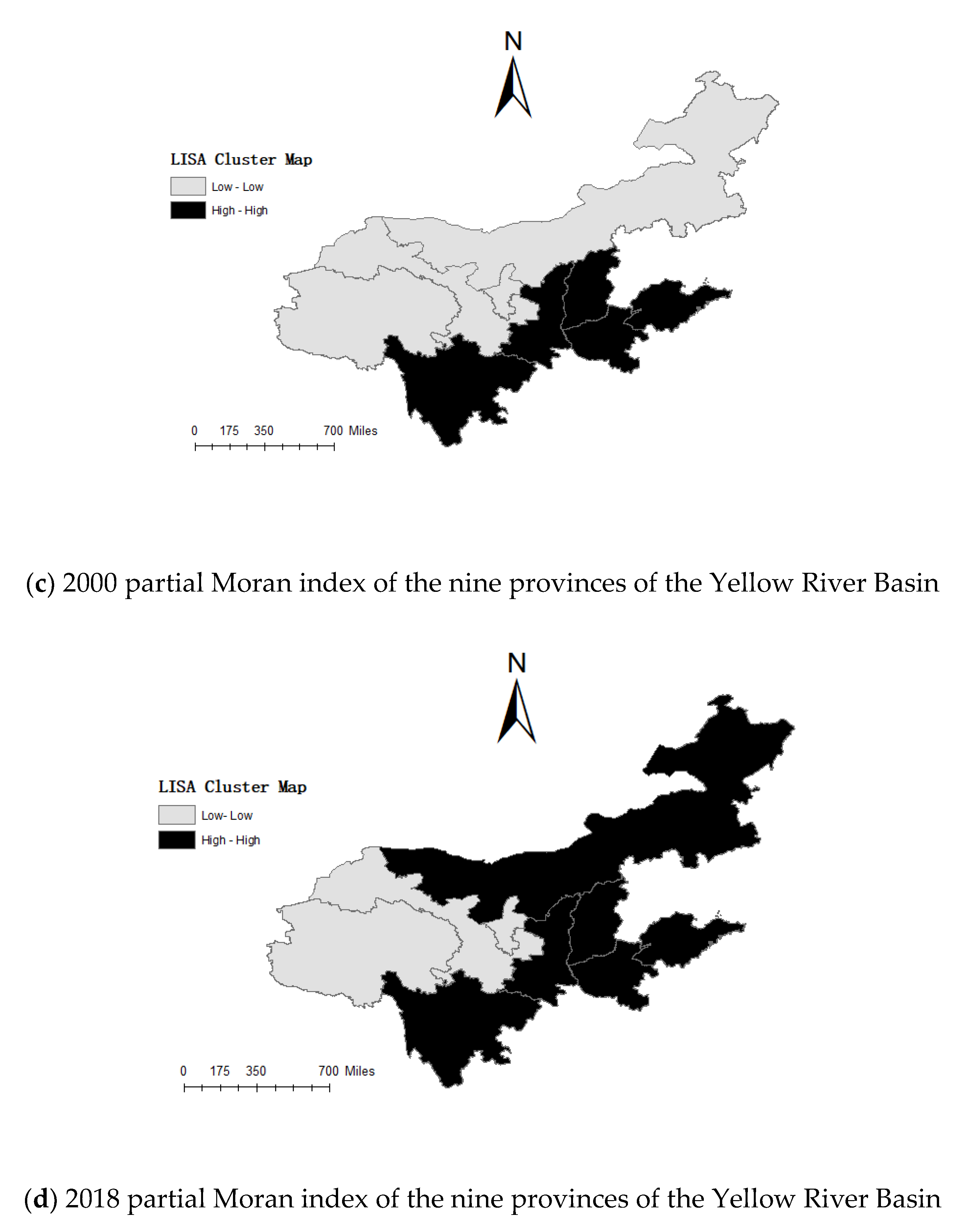
3.1.2. Local Autocorrelation Test

The Yellow River Basin has a vast area, and the topography, landforms and resource endowments of each province are quite different, which makes the economic development level and industrial structure of each province different. The global Moran’s I mentioned above is from the perspective of the overall region, reflecting the overall situation of the region, which may ignore the occurrence of heterogeneous characteristics in a local area. The local Moran’s I is an index used to measure the spatial autocorrelation of a local area. It is represented by Equation (12), and its meaning is the same as Equation (9). Compared with global Moran’s I, the local Moran’s I can make up for the above-mentioned shortcomings and thus can better describe the spatial correlation of this area.

$$I=\frac{(Y_i-\overline{Y})}{S^2}{\displaystyle \sum _{j=1}^n{w}_{ij}}(Y_j-\overline{Y})$$

(12)

Therefore, the local spatial distribution characteristics of carbon emissions in various provinces will be analyzed. Among them, the Lisa agglomeration map based on the Moran scatter plot is constructed through stata14.0, which can more intuitively reflect the agglomeration between a certain area and its neighboring areas. Due to limited space, only the agglomeration in the base period and the end period of the sample are selected as the observation objects. By comparing the local Moran scatter plots obtained under two different weight matrices, W₁ and W₂, it is found that provinces of the Yellow River Basin in 2000 and 2018 are basically distributed in the first and third quadrants. The first quadrant represents that the observation high value is surrounded by the observation high value area. The carbon emissions of the Yellow River Basin area are all higher than the average value, and the carbon emissions of the adjacent areas are also higher than the average value, showing high–high (H-H) agglomeration spatial characteristics. The third quadrant is just the opposite, which means that the observation low value is surrounded by the observation low value area, showing the characteristics of low–low (L-L) agglomeration. The first and third quadrants are both spatially positively correlated regions, which further verifies that carbon emissions have a significant positive spatial spillover effect.

Using the Lisa map drawn by Moran’s I to analyse the local agglomeration characteristics of carbon emissions. As shown from Figure 1, Shandong, Shanxi, Shaanxi, and Henan are the main high–high agglomeration areas. Vertically, under the geographic weight matrix (W₁), Inner Mongolia also joined the ranks of high emissions in 2018 compared with 2000. Under the economic–geographic weight matrix (W₂), Inner Mongolia was also added in 2018 compared to 2000. Horizontally, under two different weight matrices in 2000 and 2018, the economic–geographic weight matrix is one more Sichuan Province than the high–high agglomeration area obtained under the geographic weight matrix, which may also be related to the closer economic activities between Sichuan Province and neighboring provinces. Finally, three provinces of Gansu, Qinghai, and Ningxia have always been low–low agglomeration areas under different circumstances.

3.2. Model Estimation

The Yellow River Basin panel data from 2000–2018 are used, and the unit root test results are shown in

Table 3. Unit root test results of panel data.

Variable	LLC Test		IPS Test
	Horizontal Value	First Order Difference	Horizontal Value	First Order Difference
I	−4.428 **	−3.174 ***	−3.294 *	−3.210 **
P	−3.797 *	−5.512 ***	−3.465 *	−6.337 **
pGDP	−3.427 *	−6.723 ***	5.802	−5.651 ***
(pGDP)2	−3.126 *	−5.943 ***	1.362	−5.651 ***
T	−4.536 **	−7.487 ***	−2.607 *	−8.462 *
U	−1.790 *	−7.330 ***	−0.670	−8.042 ***
IS	7.401 *	−9.112 ***	6.060	−6.343 **

Note: *, **, and *** represent significant at the levels of 10%, 5%, and 1%, respectively.

.

At the horizontal values, the LLC tests and the IPS tests for carbon emission, population, and energy intensity all rejected the null hypothesis, indicating that the two variables were stable at the horizontal values. The LLC tests of per capita GDP, per capita GDP quadratic term, urbanization rate, and industrial structure all rejected the original hypothesis, while the IPS test all accepted the original hypothesis, indicating that the four variables were non-stable in horizontal values. Both LLC and IPS tests of industrial structure accepted the null hypothesis, indicating that it was non-stationary in horizontal values. To further test the stationarity of the seven variables, they were assigned to a first-order difference, which showed that both the LLC and IPS tests rejected the null hypothesis at the significance level, so the same-order single integration allowed a panel co-integration test between variables.

The panel consolidation test was performed using the Kao test to verify that there is a long-term equilibrium relationship between the variables. Thus, we can see that for the variables with the unit root, the stationary sequence is obtained through the first-order difference, but the economic meaning of the variables after the first-order difference is not the same as the original sequence. Given the long-term equilibrium relationship between the variables, we can still perform regression with the original sequence.

The Hausman test is used to identify the fixed-effect model or the random-effect model, and the test results are the fixed-effect model. We respectively estimated the individual fixed effect, time fixed effect, and time individual fixed effect models for the comparative analysis, and selected the most appropriate panel model for the analysis. The model fitting results are shown in

Table 4. Fixed-effect model estimates.

Variable	Individual Fixation Effect	Time Fixed Effect	Time-Based Individual Fixed-Effect model
lnIS	−0.078	0.0041 **	0.029 **
lnI	0.460 *	0.862 *	0.864 ***
(lnpGDP)2	0.013	−0.008	−0.042
lnP	0.275 **	1.269 *	1.004 **
lnT	−0.075 *	−0.156	−0.091 *
lnU	0.1538 *	0.2137	−0.106 **
R2	0.6599	0.9205	0.9417
P	0.0001	0.0002	0.000

Note: *, **, and *** represent significant at the levels of 10%, 5%, and 1%, respectively.

.

It can be found that the significance level obtained under the individual fixed effect and the time fixed effect is significantly not as good as the time individual fixed effect. Therefore, the two-fixed effect panel model is selected in this paper. Finally, Lagrange Multiplier (LM) forms LMlag, LMerr and robust LMlag (Robust LMlag) and robust LMerr (Robust LMerr) tests were applied under the geographic and spatial weight matrix, respectively. The test results are obtained under the geographical and spatial weight matrix. Therefore, the detection results under the dual fixed effect are shown in

Table 5. Spatial correlation test.

Detection Method	Economic–Geographic Weight Matrix		Geographic Weight Matrix
	Statistic	p-Value	Statistic	p-Value
$\mathrm{LMerr}$	174.647	0.000	212.227	0.000
$\mathrm{Robust} \mathrm{LMerr}$	162.567	0.000	36.045	0.000
$\mathrm{LMlag}$	12.369	0.000	181.600	0.000
$\mathrm{Robust} \mathrm{LMlag}$	0.289	0.591	5.418	0.020
Hausman test	—	0.003	—	0.000

.

The test results under geographic weight matrix and spatial weight matrix are shown in Table 5. Finally, through the joint significance test, it is known that the detection under the individual fixed effect, time fixed effect or double fixed effect model is basically the same, and it is found that the test results are basically the same. Therefore, the test results under the double fixed effect are shown in Table 5. The LMerr detection values of the geographic weight matrix and the geographic-economic weight matrix are both significant at the 1% level. The Robust LMlag detection value of the geographic-economic weight matrix failed the test, and the Robust LMlag under the geographic weight matrix was significant at the 5% level. Therefore, in comparison, the spatial error model (SEM) is more suitable for the study.

The estimated results of the fixed-effect spatial error obtained by the spatial error model under the geographic weight matrix and the geographic-economic weight matrix are shown in

Table 6. Estimated results of the spatial error fixed-effects model.

Variable	Geographic Weight Matrix	Economic–Geographic Weight Matrix
$\ln IS$	0.5837 ** (5.012)	0.6201 *** (5.982)
$\ln pGDP$	−182.3 *** (−3.927)	−201.2 *** (−5.982)
${(\ln pGDP)}^2$	20.29 *** (4.997)	24.08 ** (5.016)
$W\ast \ln I$	0.2730 *** (6.0239)	0.3219 *** (5.988)
$\ln P$	0.7231 ** (0.015)	0.5629 * (0.049)
$\ln T$	−0.075 * (0.065)	−0.156 *** (0.062)
$\ln U$	0.1538 ** (3.076)	0.2137 ** (4.274)
R2	0.9599	0.9808
Adjust R2	0.9921	0.9872
Log-L	75.58	78.37

Note: The numbers in parentheses in the table represent t-test values, *, **, and *** represent significant at the levels of 10%, 5%, and 1%, respectively.

.

As shown in Table 6, the fitting effect of the spatial error fixed-effects model is better than in Table 5. The economic–geographic weight matrix is compared with the geographic weight matrix, and the goodness of fit and log likelihood of the former are slightly larger than the latter in Table 6. This also shows that the fitting effect of the economic–geographic weight matrix that nests economic factors and geographic factors together is better than that of the geographic weight matrix which only considers geographic factors. Meanwhile, the result also shows that the economic activities between provinces also have obvious spatial dependence. In addition, the explanatory variables and the explained variables in the regression results are mostly significant at the levels of 1% and 5%, which also shows that economic growth and industrial structure will have a more significant impact on carbon emissions.

3.3. Comparative Analysis of Spatial Spillover Effects of Carbon Emissions in the Yellow River Basin and the Yangtze River Basin

Both the Yangtze River Basin and the Yellow River Basin are the birthplaces of Chinese civilization. The parallel analysis of the two major river basins will help us better deal with the problem of increased carbon emissions in the two major river basins.

3.3.1. The Current Status of Carbon Emissions in the Yellow River Basin and the Yangtze River Basin

By calculating the carbon emissions of the two major river basins, it is found that carbon emissions of the Yangtze River Basin are significantly higher than that of the Yellow River Basin. At the same time, the carbon emissions in the Yangtze River Basin have shown a tendency to increase first and then decrease. Although carbon emissions in the Yellow River Basin are significantly lower than those in the Yangtze River Basin, it has continued to grow. A detailed graph of the carbon emissions change trend of the two major river basins is drawn in Figure 2.

3.3.2. The Spatial Spillover Effect of Carbon Emissions in the Yangtze River Basin

Using the above analysis ideas, this paper uses the economic–geographic weight matrix to perform the same analysis on the spatial effects of the Yangtze River Basin. First, we conduct a spatial correlation test on the carbon emissions of the provinces in the Yangtze River Basin. And learned that Moran’s I of carbon emissions are all significantly positive, which also shows that there is a significant positive spatial autocorrelation of carbon emissions in the provinces of the Yangtze River Basin. Then, through the $LM$ test and the robust $LM$ test results, the $LM$ test and the robust $LM$ test of the spatial error panel model are significant at the 1% level. But the test results of the spatial lag panel model failed, which shows that the spatial error panel model is more reasonable. The conclusion further shows that the growth of carbon emissions in the provinces of the Yangtze River Basin is not only caused by various economic and social factors, but also affected by neighboring provinces. Finally, the data of the Yangtze River Basin is significant at the 1% level by Hausman test, so the fixed effects model is selected. And the test results are shown in

Table 7. Statistical Test of SLPDM and SEPDM.

Variable	Statistics	p-Value
$\mathrm{LMerr}$	167.41	0.000
$\mathrm{Robust} \mathrm{LMerr}$	162.38	0.002
$\mathrm{LMlag}$	6.35	0.128
$\mathrm{Robust} \mathrm{LMlag}$	0.57	0.213
Hausman	—	0.000

.

The estimation results of the spatial panel model in the Yangtze River Basin are shown in

Table 8. Estimated results of the Yangtze River Basin model.

Variable	Statistics	p-Value
$\ln IS$	0.34	0.067
$\ln pGDP$	0.29	0.001
${(\ln pGDP)}^2$	−0.14	0.000
$W\ast \ln I$	0.22	0.000
$\ln P$	0.79	0.004
$\ln T$	0.16	0.001
$\ln U$	0.07	0.040
R2	0.8902
Log-L	302.71

. The industrial structure, population size, energy intensity, and urbanization level all have significant positive impacts on carbon emissions in the Yangtze River Basin. The $\ln pGDP$ coefficient is significantly positive at the 1% level, and its quadratic coefficient is significantly negative, which also shows that the EKC curve of the spatial panel model of carbon emissions in the Yangtze River Basin is valid and presents an inverted “U”-shaped curve relationship.

3.4. Results of Empirical Analysis

3.4.1. Spatial Effect of Carbon Emissions

According to the estimation results of spatial error fixed effect model, the carbon emission of provinces and regions in the Yellow River Basin has obvious spatial spillover effect. The spatial autocorrelation coefficient $\rho$ is significantly positive under both the geographic spatial weight matrix and the economic geographic weight matrix, that is, regardless of the nested measurement of economic development and geographic distance, or the neighboring conditions, the results show that the carbon emissions of various provinces are Change in the same direction. At the same time, according to the Lisa map analysis in Figure 1, it is found that the carbon emissions of various provinces show positive spatial correlation characteristics. Among which, the high–high carbon emission areas are mainly distributed in Shandong, Shaanxi, Shanxi, Henan, Inner Mongolia, Sichuan and other provinces, and the low–low carbon emission areas are mainly in Gansu, Qinghai, and Ningxia. The carbon emission spatial spillover effect of high–high agglomeration, namely the phenomenon of “pollution refuge”, is caused by two reasons: Firstly, carbon emissions have a certain diffusion effect. Secondly, the close relationship between economic activities cannot be ignored. Therefore, all provinces should formulate carbon emission reduction measures from the perspective of coordinated development.

3.4.2. Analysis of Influence Factors

In terms of economic growth, the first-order coefficient of logarithm of per capita GDP is significantly negative, and the quadratic coefficient is significantly positive, which shows that there is an obvious “U”-shaped EKC curve relationship between carbon emissions and economic growth. In this process, an inflection point appears. Before the inflection point, carbon emissions decrease with economic growth. After the inflection point, carbon emissions increase with economic growth, which may be due to the Yellow River Basin’s long-term dependence on energy-intensive industries to promote economic growth. At the same time, the economic growth of this region does not rely entirely on its own strength. It will be affected by the spillover effects of neighboring provinces and cities. Under the vision of “carbon peak and carbon neutral”, the primary task of all provinces and regions is to change the status quo of the secondary industry as the main grow engine.

In terms of industrial structure, the impact of industrial structure on carbon emissions is significantly positive in both geographical weight matrix and economic–geographical weight matrix. Under the economic–geographic weighting matrix, its estimated coefficient is 0.6201, which means that for every 1% increase in the proportion of the secondary industry in the GDP, the increase in carbon emissions dropped to 0.6201%. This is also related to the current extensive industrialization development model of the Yellow River Basin and the secondary industry-based industrial structure in Shandong, Shanxi. Therefore, under the circumstance that other conditions remain unchanged, provinces dominated by secondary industries will have higher carbon emissions levels, and will also affect the carbon emissions level of neighboring provinces or related provinces with close economic ties to the province. Therefore, in order to achieve the goal of carbon emission reduction, all provinces should actively adjust the industrial structure, vigorously develop the tertiary industry, and reduce the proportion of the secondary industry.

The population size can reflect the impact of population density on the environment to a certain extent. In general, the larger the population, the higher the population density in a certain area, the higher the demand for energy and the greater the pressure on the environment. It can be seen from Table 3 that the population size coefficients under the two spatial weight matrices are significantly positive, which also verifies the previous guess that an increase in population size will lead to an increase in carbon emissions.

The level of technological development has various effects on carbon emissions. On the one hand, the rapid economic development has made people pay more attention to the quality of life and living environment, change the original lifestyle, and adopt a low-carbon lifestyle, which has led to a reduction in carbon emissions. On the other hand, the reduction in carbon emissions brought about by technological progress may not be enough to offset the increase in carbon emissions, resulting in a positive impact on carbon emissions by technological level. Under different weighting matrices, the level of technological development has a negative impact on carbon emissions, which means that the negative impact of technological progress on carbon emissions during the sample period is greater than the positive impact of technological progress on carbon emissions.

From the perspective of the level of urbanization, the development of urbanization in the Yellow River Basin is also one of the important factors causing the increase in carbon emissions. Although all provinces are actively increasing the green area and working hard to increase carbon absorption. However, the environmental pressure brought about by the rapid development of urbanization level still aggravates carbon emissions.

It is worth noting that the industrial structure, population size, energy intensity, and urbanization level of the Yangtze River Basin have a significant positive impact on carbon emissions. At the same time, there also exists an inverted “U”-shaped curve relationship between carbon emissions and economic growth. In other words, economic growth will cause carbon emissions to increase first and then decrease, which is in contrast with the analysis results of the Yellow River Basin.

This section may be divided by subheadings. It should provide a concise and precise description of the experimental results, their interpretation, as well as the experimental conclusions that can be drawn.

4. Conclusions and Recommendations

4.1. Conclusions

Within the Yellow River Basin, carbon emissions from neighboring provinces or provinces with close economic and trade activities present a strong spatial agglomeration feature; Moreover, the carbon emissions among most provinces show a high–high concentration phenomenon, that is, the increase of carbon emissions will increase the carbon emissions of neighboring provinces or provinces with similar economy and geography. In the economic–geographical weight matrix, there are more high–high-cluster regions than those in the geographical weight matrix, which further indicates that economic activities also present a relatively significant spatial effect. Shandong, Shanxi, Shaanxi, Henan, Inner Mongolia and Sichuan are high–high agglomeration regions, while Gansu, Qinghai and Ningxia are low–low agglomeration regions.

There is a “U” -shaped environmental Kuznets curve relationship between economic growth and carbon emissions. The primary coefficient of per capita GDP is negative, while the quadratic coefficient is positive, indicating that economic growth and carbon emissions present a “U” -shaped environmental Kuznets curve relationship. There is a significant spillover effect among the carbon emissions of provinces in the Yellow River Basin. Specifically, in the economic–geographical weight matrix, each 1% increase in carbon emissions of neighboring provinces will increase the carbon emissions of the region by 0.3219%. Industrial structure also shows a significant positive impact on carbon emissions. In the economic–geographical weight matrix, its estimated coefficient is 0.6201, which means that when the proportion of the secondary industry in the GDP increases by 1%, the increase in carbon emissions dropped to 0.6201%. The coefficient of population size is negative, which also indicates that the increasing population also leads to the increase of carbon emissions. At the same time, the level of urbanization is also one of the important factors causing the increase of carbon emissions. The level of technological development is significantly negative under the two weight matrices, in other words, the total carbon emission can be reduced by technological progress.

The positive “U”-shaped relationship between economic growth and carbon emissions in the Yellow River Basin is significantly in contrast to the inverted “U” -shaped relationship between economic growth and carbon emissions in the Yangtze River Basin. The industrial structure, population size, energy intensity and urbanization level of the Yangtze River Basin all have a significant positive impact on carbon emissions. At the same time, there is an inverted “U” curve relationship between carbon emissions and economic growth, that is, economic growth will make carbon emissions first increase and then decrease, which further shows that the Yellow River basin is still an extensive economic growth model, which is different from that in the Yangtze River basin.

4.2. Recommendations

Based on the above conclusions, the following suggestions were put forward:

The spatial spillover effect of carbon emissions makes carbon emission reductions very ineffective. The joint prevention and control mechanism in the Yellow River Basin should be promoted to reduce spillover effects in high-emission provinces. Related apartments should strictly control the phenomenon of “pollution transfer”, and develop green industries suited to local conditions, rather than taking on high-polluting industries from neighboring provinces. For example, Qinghai Province can rely on its own high-altitude advantages to focus on the development of hydropower projects, conduct in-depth green surveys of strategic resources, and deepen the research, the development and utilization of clean energy. In short, to achieve the high-quality development of the Yellow River Basin, all regions are required to strictly follow the “two mountains” theory as guiding ideology and find new ways to give full play to their own advantages.

The mode of economic growth should be transformed, and the development of the green service industry should be promoted. The positive “U”-shaped relationship between economic growth and carbon emissions in the Yellow River Basin is in marked contrast with the inverted “U”-shaped relationship between economic growth and carbon emissions in the Yangtze River Basin, which further shows that the Yellow River Basin is still an extensive economic growth model. Therefore, we must actively guide the development and prosperity of the green industry. The purification capacity and carrying capacity of the environment are limited. A series of environmental problems such as global warming and climate deterioration are all “warnings” of nature to mankind. Each of the nine provinces of the Yellow River has put forward the “14th Five-Year” energy development plan and formulated energy conservation and emission reduction targets. Among which, transforming the mode of economic growth, persisting in the orientation of green development, strictly adhering to the “three lines and one order”, and implementing green transformation of key industries are the top priorities of the energy development plan. At the same time, as one of the cradles of Chinese civilization, the Yellow River Basin has abundant innovation resources and innovation potential, which are the basic forces that promote technological innovation and economic growth. It is of vital importance to help improve energy efficiency and realize a true low-carbon economy.

The optimization and upgrading of the industrial structure, and dynamically dealing with the relationship between the industrial structure and carbon emissions should be strived to improve. It is difficult to meet the challenges of economic development by only relying on high energy-consuming and high-polluting secondary industries. The low added value of the secondary industry is difficult to take advantage of the economic development of the Yellow River Basin.

For example, Shanxi Province has always relied on electricity prices as a development advantage due to its rich resources such as coal. However, under the background of rapid development of new kinetic energy, resource advantages are becoming less obvious. Therefore, the government should further promote the green and intelligent mining of coal mines, promote the optimized utilization of coal by quality and cascade, and do a good job in policies for coal use reduction and for replacing some coal use with alternative energy sources. The government should also improve the electricity spot-market trading system and improve the electricity price mechanism for strategic emerging industries. Comparing the rapid development of the tertiary industry based on the service industry in various regions of the Yangtze River Basin, the industrial structure of the secondary industry of some provinces in the Yellow River Basin is too low to match. At the same time, when planning the industrial structure, local governments should also pay attention to the spatial spillover effect of industrial agglomeration carbon emission reduction, and establish and improve cross-regional and cross-border cooperation mechanisms.

The government should strictly implement differentiated emission reduction policies. The Yellow River Basin is vast, and there are certain differences in the economic development and resource content of different regions, which make the impact of economic growth and industrial structure on carbon emissions in different regions of different periods or in different regions of the same period significantly heterogeneous. Therefore, in order to achieve the high-quality development of the Yellow River Basin and for China’s “carbon neutral” goal, the local government should clarify their respective emission reduction targets and share effective policies together.

References

1. Cramer, J.C. A demographic perspective on air quality: Conceptual issues surrounding environmental impacts of population growth. Hum. Ecol. Rev. 1997, 3, 191–196. [Google Scholar]
2. York, R.; Rosa, E.A.; Dietz, T. Stirpat, ipat and impact: Analytic tools for unpacking the driving forces of environmental impacts. Ecol. Econ. 2003, 46, 351–365. [Google Scholar] [CrossRef]
3. Luo, Y.L.; Zeng, W.L.; Hu, X.B.; Yang, H.; Shao, L. Coupling the driving forces of urban CO2 emission in Shanghai with logarithmic mean Divisia index method and Granger causality inference. J. Clean. Prod. 2021, 298, 126843. [Google Scholar] [CrossRef]
4. Wang, M.; Arshed, N.; Munir, M.; Rasool, S.F.; Lin, W. Investigation of the STIRPAT model of environmental quality: A case of nonlinear quantile panel data analysis. Environ. Dev. Sustain. 2021, 23, 12217–12232. [Google Scholar] [CrossRef]
5. Chen, X.; Zhou, P. Empirical Study on Carbon Emission Level of China (Relying on FDI) Participating in International Industrial Transfer. Ecol. Econ. 2020, 149, 112050. [Google Scholar]
6. Hu, Y.; Zhang, X.W.; Li, J. Export, Geography Conditions and Air Pollution. China Ind. Econ. 2019, 94, 98–116. [Google Scholar]
7. Li, Y.H. Measure of the impact of fiscal decentralization on carbon emissions based on the STIRPAT model. Stat. Decis. 2020, 19, 136–140. [Google Scholar]
8. Arshed, N.; Munir, M.; Iqbal, M. Sustainability assessment using STIRPAT approach to environmental quality: An extended panel data analysis. Environ. Sci. Pollut. Res. 2021, 28, 18163–18175. [Google Scholar] [CrossRef]
9. Sun, X.; Zhang, H.; Ahmad, M.; Xue, C. Analysis of influencing factors of carbon emissions in resource-based cities in the Yellow River basin under carbon neutrality target. Environ. Sci. Pollut. Res. 2021, 28, 1–14. [Google Scholar] [CrossRef]
10. Burnett, J.W.; Bergstrom, J.C.; Dorfinan, J.H. A spatial panel data approach to estimating U.S. state-level energy emissions. Energy Econ. 2013, 40, 396–404. [Google Scholar] [CrossRef]
11. Li, J.; Li, S. Energy investment, economic growth and carbon emissions in China—Empirical analysis based on spatial durbin model. Energy Policy 2020, 140, 111425. [Google Scholar] [CrossRef]
12. Chen, W.; Peng, Y.; Yu, G. The influencing factors and spillover effects of interprovincial agricultural carbon emissions in China. PLoS ONE 2020, 15, 0240800. [Google Scholar] [CrossRef] [PubMed]
13. Wang, Z.; Wang, C.; Yin, J. Strategies for addressing climate change on the industrial level: Affecting factors to co2 emissions of energy-intensive industries in China. Nat. Hazards 2015, 75, 303–317. [Google Scholar] [CrossRef]
14. Xue, L.M.; Meng, S.; Wang, J.X.; Liu, L.; Zheng, Z.X. Influential Factors Regarding Carbon Emission Intensity in China: A Spatial Econometric Analysis from a Provincial Perspective. Sustainability 2020, 12, 8097. [Google Scholar] [CrossRef]
15. Wu, S.; Hu, S.; Frazier, A.E. Spatiotemporal variation and driving factors of carbon emissions in three industrial land spaces in China from 1997 to 2016. Technol. Forecast. Soc. Change 2021, 169, 120837. [Google Scholar] [CrossRef]
16. Yang, X.; Jia, Z.; Yang, Z.; Yuan, X. The effects of technological factors on carbon emissions from various sectors in China—A spatial perspective. J. Clean. Prod. 2021, 301, 126949. [Google Scholar] [CrossRef]
17. Tong, X.; Salman, T. The Spatiotemporal Evolution Pattern and Influential Factor of Regional Carbon Emission Convergence in China. Adv. Meteorol. 2020, 25, 2142–2153. [Google Scholar] [CrossRef]
18. Wen, L.; Li, Z.K. Driving forces of national and regional CO2 emissions in China combined IPAT-E and PLS-SEM model. Sci. Total Environ. 2019, 690, 237–247. [Google Scholar] [CrossRef]
19. Wei, Y.G.; Zhu, X.H.; Li, Y.; Tao, Y. Influential factors of national and regional CO2 emission in China based on combined model of DPSIR and PLS-SEM. J. Clean. Prod. 2019, 212, 698–712. [Google Scholar] [CrossRef]
20. Miao, J.J.; Hua, C.; Feng, J.C. Upgrading Effect of Industrial Collaborative Agglomeration and Carbon Emission: An Empirical Analysis Based on and Carbon Emission: An Empirical Analysis Based on. Ecol. Econ. 2020, 36, 28–33. [Google Scholar]
21. Sun, J.W.; Yao, P. The research paradigm and recent progress of space econometrics. Economist 2014, 9, 27–35. [Google Scholar]
22. Hang, Y.; Wang, Q.; Zhou, D.; Zhang, L. Factors influencing the progress in decoupling economic growth from carbon dioxide emissions in China’s manufacturing industry. Resour. Conserv. Recycl. 2019, 146, 77–88. [Google Scholar] [CrossRef]
23. Zhao, G.M.; Geng, Y.; Sun, H.P.; Zhao, G.Q. Spatial effects and transmission mechanism of inter-provincial Spatial effects and transmission mechanism of inter-provincial China Population. Resour. Environ. 2020, 27, 49–55. [Google Scholar]
24. Liu, Y.Y.; Wang, Y.Q.; An, R.; Li, C. The spatial distribution of commuting CO2 emissions and the influential factors: A case study in Xi’an, China. Adv. Clim. Change Res. 2015, 6, 46–55. [Google Scholar] [CrossRef]
25. Li, J.; Tan, Q.M.; Bai, J.H. Space Measurement Analysis of China’s Regional Innovation Production: An Empirical Study Based on Static and Dynamic Space Panel Models. Manag. World 2010, 7, 43–45. [Google Scholar]
Figure 1. The Moran’s I in nine provinces of the Yellow River Basin in 2000 and 2018.
Sustainability 14 03608 g001aSustainability 14 03608 g001b
Figure 2. Trends of carbon emissions in the two major river basins.
Sustainability 14 03608 g002