A Two-Stage Planning Optimization Study of an Integrated Energy System Considering Uncertainty

Abstract

In the context of a rapidly evolving integrated energy system (IES), taking into account the uncertainty of the renewable energy output can make integrated energy system planning more realistic. In view of this, this paper proposes an integrated energy system planning approach that takes uncertainty into account. Firstly, in order to accurately describe the renewable energy output scenarios, this paper describes the IES model and introduces the scenario analysis methods used. Secondly, an integrated energy system equipment output model is constructed, the corresponding constraints and objective functions are set, an improved particle swarm-ant colony optimization algorithm is used for the solution, and a planning solution strategy considering uncertainty is proposed. Finally, the above conclusions are verified by the actual case data of a park, and the results show that the method proposed in this paper is economical and reasonable.

1. Introduction

1.1. Problem Statement

As the lifeblood of the national economy, energy issues will directly affect the progress and development of society. In the face of rising global energy consumption, the shortage of traditional energy sources, the low efficiency of energy utilization in traditional energy supply systems, the gradual strictness of national requirements for energy conservation and environmental protection, and the new energy situation of the large-scale application and development of renewable energy, the establishment of a green, low-carbon, energy-saving, and environmentally friendly; safe; and efficient energy system is an important direction for energy transformation and development. In 2020, China proposed a “double carbon target”, which puts forward new requirements for energy development, and the transformation and development of the energy system is necessary to achieve this target [1].

In recent years, with the promotion of concepts such as integrated energy systems and the energy internet, the energy industry has continued to develop towards efficient, safe, and sustainable energy use [2]. With the increase in electrification and the advancement of “electrical energy substitution” technologies, various energy sources are interconnected through different coupling links, breaking the pattern of independent planning and operation of energy supplies such as electricity, heat, cooling, and natural gas. The coupling between the electricity network and energy systems is becoming increasingly close [3].

The integrated energy system integrates a multi-energy flow network of cooling, heating, electricity, and gas, with complex relationships between the multi-energy coupling equipment within the system, making it a complex energy system with a multi-energy flow input and output. The scientific and reasonable planning of the integrated energy system is the basis for the development of integrated energy projects, which directly affects the realization of the advantages of the system, such as high efficiency and economic and environmental protection. Renewable energy generation equipment, as an important part of an integrated energy system, has a continuously changing output due to changes in solar irradiance and wind speed, which leads to uncertainty in the power system. Therefore, these resource uncertainties should be taken into account when planning for integrated energy systems.

1.2. Literature Survey

The scientific and rational planning of integrated energy systems is the basis for the development of integrated energy projects and has a direct impact on the realization of the advantages of efficient, economic, and environmentally friendly systems. Therefore, a number of scholars have carried out extensive research around the planning of integrated energy systems, mainly focusing on the modelling of planning methods, equipment capacity configuration, system uncertainty, and other aspects.

In terms of the planning and optimization of integrated energy systems, reference [4] proposed a method for planning and optimizing integrated energy systems by combining multiple factors of demand. Based on the demand data of an industrial park, the method was applied to complete a case study of integrated energy system planning, which verifies the feasibility and effectiveness of the method. Reference [5] designed an optimization method for energy management of integrated community energy systems based on user-led demand-side response to improve the robustness of the scheduling model under different forecasting accuracies by introducing advance IDR bidding and the conditional value-at-risk (CVaR) theory. In [6], a hierarchical management strategy for regional multi-energy systems was designed, using a consensus algorithm to determine the proportion of the distributed distribution of electricity and natural gas exported or imported from each DMES, effectively improving the resilience of the integrated energy distribution system. Reference [7] takes into account the objectives of reducing system active losses, increasing profitability and enhancing stability when planning the optimization of distributed generating units and designing the corresponding models for their solution. In [8], a capacity allocation method for CCHP units, auxiliary boilers, and electric de-heating equipment was proposed for a hotel in Tehran as an example to achieve optimal planning of a small CCHP system.

Integrated energy planning involves many factors and is subject to a variety of uncertainties when it comes to optimal allocation. On the one hand, demand on the customer side is diverse and subject to uncertainty and randomness due to external factors such as seasonal and diurnal changes, and on the other hand, renewable energy generation systems have poor power stability and uncertainty. In order to consider the impact of uncertainty factors on system planning, scholars at home and abroad have carried out relevant research. Reference [9] used a scenario analysis to model the uncertainties arising from renewable energy output and load demand, and it proposed a low carbon optimization model. Reference [10] used a stochastic planning approach combined with a multi-scenario approach to develop an uncertainty planning model considering wind power generation and load forecasting, and it introduced scenario reduction techniques to reduce the computational burden of the model. Reference [11] provides a scenario-based evaluation strategy for integrated energy system planning by simultaneously considering uncertain parameters (electricity price and wind turbine output power) and carbon capture utilization and storage (CCUS) technology. Reference [12] presents a multi-stage robust optimization model for the coordinated operation of a coupled electricity–gas–transport system that takes into account uncertainties in traffic demand, wind power, and gas consumption of gas units simultaneously. Reference [13] describes the price uncertainty as a normal distribution and develops a two-stage stochastic planning model with investment planning as the first-stage problem and IES operation as the second-stage problem through a multi-scenario simulation.

From the above literature, it can be found that a scenario analysis is commonly used as an effective method to solve power system problems involving wind and light uncertainties. Reference [14] proposed a multi-objective joint planning model for active distribution networks, using a scenario stochastic modelling approach based on the Wasserstein distance metric and a K-medoids scenario analysis to effectively model the stochastic nature of renewable energy generation. Reference [15] modelled uncertainty in the output power of PV systems and wind turbines, load demand forecast errors, and grid bid changes through a scenario analysis approach for optimal energy management of microgrids. In [16], a short-term stochastic optimization model for a hybrid water–wind–photovoltaic system was constructed, using an integrated forecasting and scenario tree approach to achieve a comprehensive simulation of the uncertainty in renewable energy production and load demand. In [17], a new hybrid copula-scenario-based uncertainty modelling technique was proposed to improve the energy management of microgrids by considering the uncertainties of wind, solar, market clearing price (MCP), and load. Reference [18] proposes an optimal stochastic dispatch model for energy hubs combined with P2G storage, applying a scenario-based stochastic approach to deal with uncertainties associated with electricity loads, wind power, and tariffs, and the results of the arithmetic examples confirm that the proposed approach substantially reduces operating costs by about 7%.

1.3. Contribution of This Paper

In summary, the presence of uncertainty factors in integrated energy system planning can have an impact on the system. Some of the studies on the consideration of uncertainty factors are relatively simple and only focus on load uncertainty, while renewable energy, as an important input to integrated energy, needs to be considered in the planning stage. Therefore, this paper proposes an integrated energy system planning method that takes uncertainty into account, with the following main innovations:

(1)

A non-parametric probabilistic forecasting method is used to generate typical output scenarios for renewable energy generation equipment, and the scenarios are reduced using an improved k-means clustering algorithm to improve the accuracy of the integrated energy system planning scenarios.

(2)

This paper designs an integrated energy system planning solution strategy that takes into account uncertainty factors; the scenario analysis is combined with the solution strategy to obtain integrated energy equipment capacity planning configuration results for different scenarios.

(3)

An improved particle swarm-ant colony optimization algorithm is proposed, combining the advantages of fewer particle swarm parameters with the ant colony algorithm, taking into account the advantages of the robustness of the ant colony algorithm and increasing the solution speed of the algorithm by reducing the number of algorithm parameters to be adjusted.

(4)

This paper presents a case study based on the characteristics of the output of clean energy equipment and the behavioral characteristics of the user side of an industrial park in southern China. The results show that the integrated energy planning approach proposed in this paper can effectively cope with the uncertainty of the output of wind and light, and it can take into account various needs such as the economy, stability, and security.

2. Materials and Methods

2.1. Typical Structure of an IES

An integrated energy system is an extremely complex energy coupling system containing multiple functions, including energy input, conversion, and output. The prerequisite for planning and optimizing the IES is to establish an accurate and scientific framework for the IES. A typical IES consists of four links, which are source, network, load, and storage. The main sources of energy input to the system are wind, solar, water, and natural gas. The converted energy sources at the user end are electricity, heat, and cold. The system can convert energy into the form of energy we need through different energy conversion devices and delivery networks. Typical devices in the system are a gas turbine, gas boilers, refrigeration units, and lithium bromide. In addition, the system includes energy storage facilities to store and release excess energy for the purpose of improving energy efficiency. In addition, the system includes energy storage facilities to store and release excess energy for the purpose of improving energy efficiency. There are also studies that refer to integrated energy systems as Energy Hub and Multicarrier Energy Systems, as they all perform the same function of the efficient use of all types of energy and use the same equipment and devices

IES has a wide variety of energy sources, including a large number of renewable energy sources, and the system needs to maintain a real-time balance between the source and load sides. However, wind turbine power generation and photovoltaic power generation output has strong uncertainty and randomness, and the prediction accuracy is low and not easy to control and predict, which also indirectly leads to the uncertainty of cool, thermal, and electric loads at the customer side of the IES.

2.2. Wind Turbine and PV Output Model

Since renewable energy comes mainly from solar and wind, it is easily disturbed by more factors such as temperature, environment, and season, and we cannot predict and control it accurately. Therefore, this uncertainty of the wind turbine and PV output is also one of the manifestations of the scenario, but the light intensity and wind power can be regarded as some kind of functional distribution. In this paper, we will start from the probability density of the wind turbine and PV power output and focus on the power output of the equipment.

2.2.1. Photovoltaic Power Generation Equipment

The light intensity in a certain time period can be approximated as a functional distribution with a probability density distribution function as shown in Formula (1).

$$f\left(s\right)=\frac{\mathsf{\Gamma }\left(\alpha ,\beta \right)}{\mathsf{\Gamma }\left(\alpha \right)\mathsf{\Gamma }\left(\beta \right)}{\left(\frac{s}{s_m}\right)}^{\alpha -1}{\left(1-\frac{s}{s_m}\right)}^{\beta -1}$$

(1)

In the formula, $s$ and $s_m$ are the actual and maximum light intensity. $\alpha$ and $\beta$ are Beta distribution parameters, and $\mathsf{\Gamma }$ is the Gamma function. The output power of the PV panel is calculated according to the following Formula (2):

$$P_{pv}=s\cdot \psi \cos \left(\theta \right){\eta }_V{A}_V{\eta }_{vp}$$

(2)

In the formula, ${\eta }_V$ is the efficiency coefficient of the “maximum power point tracking” solar controller. ${\eta }_{vp}$ is the efficiency coefficient of the PV cell. $A_V$ is the panel area. $\psi$ and $\theta$ are the solar radiation and solar incidence angle, respectively.

2.2.2. Wind Turbine Power Generation Equipment

We assume that the power generated by the wind turbine follows a normal distribution $N\left(\mu ,{\delta }^2\right)$. Its probability density distribution function can be expressed as Formula (3):

$$f\left(v\right)=\sqrt{\frac{1}{2\pi \sigma }}\exp \left[-\frac{{\left(v-\mu \right)}^2}{2{\sigma }^2}\right]$$

(3)

In the formula, parameter $\mu$ is the expected value, parameter ${\sigma }^2$ is the variance, and $v$ is the wind speed.

Based on the probability density of wind speed, the wind turbine output power can be obtained, as shown in Formula (4):

$$P_{wt}=\{\begin{array}{l}\hspace{1em}\hspace{1em}0\hspace{1em}\hspace{1em}\hspace{1em}\hspace{1em}v<v_{ci}\\ a_v{v}^2+b_{v}v+c_v\hspace{1em}{v}_{ci}\le v<v_r\\ \hspace{1em}\hspace{1em}{P}_{wt\underset{\_}{}r}\hspace{1em}\hspace{1em}\hspace{1em}{v}_r\le v<v_{co}\\ \hspace{1em}\hspace{1em}0\hspace{1em}\hspace{1em}\hspace{1em}\hspace{1em}\hspace{1em}v\ge v_{co}\end{array}$$

(4)

In the formula, $v_{ci}$, $v_{co}$, and $v_r$ are cut-in power speed, cut-out power speed, and rated power speed, respectively. The coefficients $a_v$, $b_v$, and $c_v$ are the wind turbine output coefficients.

2.3. Scenario Analysis Methods

Renewable energy generation exhibits strong randomness, intermittency, volatility, and unpredictability, and this uncertainty also brings great difficulties to the scheduling and operation of energy supply systems. Therefore, in the planning and operation of integrated energy systems considering renewable energy access, how to reasonably and accurately analyze the uncertainty of renewable energy to improve the safety and reliability of the system is a problem that must be solved.

Traditional research often uses parametric forecasting methods in probabilistic forecasting methods, assuming that the forecast target obeys a specific distribution form, training the parameters of the pre-assumed distribution model based on historical data, and then making forecasts. On this basis, the planning and operation of the power system is solved, but the exact probability distribution characteristics of renewable energy sources, such as wind power, are often difficult to obtain, and the probabilistic models built have certain errors that do not guarantee the validity of the results.

Non-parametric forecasting methods do not make assumptions about the form of the distribution of the forecast target and can effectively avoid modelling errors associated with the choice of the model distribution form. More mature non-parametric methods include quantile point regression transmission and adaptive resampling methods, but the probabilistic forecasting models of these methods do not systematically consider the boundary constraint that the wind power must satisfy the value taken within the installed capacity of the wind farm. This paper proposes a non-parametric probabilistic prediction method based on kernel density estimation, which improves the probabilistic prediction accuracy while taking into account the boundary constraint of wind power, making the prediction results more realistic.

2.3.1. Scenario Generation

The first thing to do when planning multiple scenarios for the IES is to determine the types of uncertainties contained within the scenario, such as the type of energy source, level of load variation, and other influencing factors. A reasonable statistical method is used to determine the range of values of these factors, and these values are combined and matched with each other to obtain the set of all scenarios. Suppose there is a plan $\beta$ containing a total of $n$ uncertainty factors, where the $ith$ uncertainty factor has $m_i$ possible values, then the number of scenarios for this plan is shown in Formula (5):

$$M=m_1\times m_2\times m_3\dots m_n$$

(5)

If the probability of occurrence of the $p$ possible value of the $ith$ uncertainty factor is ${\phi }_{ip}$, the scenario $\sigma$ takes the following values: the $k_n$ possible value of the $n$ uncertainty. The probability of scenario generation is given in Formula (6).

$${\alpha }_{\sigma }={\displaystyle \prod _{i=1}^n{\phi }_{i{k}_i}}$$

(6)

In addition, assuming that the costs of the planning scenario of the project in different scenarios are $C_1$, $C_2$, $C_3$, …$C_M$, then the cost expectation of the scenario is shown in Formula (7):

$$E\left(C\right)={\displaystyle \sum _{\sigma =1}^M{C}_{\sigma }{\alpha }_{\sigma }}$$

(7)

If cost $C$ is a continuous random variable and the probability density function is $f\left(C\right)$, one can assume the existence of a mathematical expectation $E_2\left(C\right)$.

$$E_2\left(C\right)={\displaystyle \underset{-\infty }{\overset{\infty }{\int }}C}f\left(C\right)dx$$

(8)

This paper mainly adopts a non-parametric probabilistic prediction method for scenario generation, which is characterized by the ability to predict possible scenarios in the future time period based on the historical data of the studied scenarios, as well as to analyze and value the existence of some characteristics of the scenarios. An important part of the nonparametric probabilistic prediction method, namely nonparametric probability density estimation, and kernel density, as a commonly used estimation method, is described as follows.

Suppose that $L(•)$ is a given probability density function on N. $h_c$ is called the window width, and $\underset{c\to \infty }{\lim }{h}_c=0$ and is a constant.

$$f_c\left(x\right)=\frac{1}{c{h}_c}{\displaystyle {\sum }_{i=1}^{c}L\left(\frac{X_I-x}{h_c}\right)}$$

(9)

In the formula, $f_c\left(x\right)$ is said to be the kernel estimate of the density function $f\left(x\right)$, also called the kernel density estimate, and in this formula, $L(•)$ is the kernel function.

2.3.2. Scenario Reduction

Since the scenario data containing wind and light are characterized by high volatility and large computation, in order to make the scenario clustering faster and more efficient, this paper proposes an improved K-means clustering algorithm, which solves some defects of the traditional clustering algorithm, such as not being able to calculate the optimal number of clusters and longer computation time.

Assuming that the total number of samples in the dataset is $N$, the search range for the number of clusters can be calculated to be an integer within $\left[2,\sqrt{N}\right]$. In this paper, the PFS index is chosen as a different evaluation index for clustering results, as defined in Formula (10).

$$PFS=\frac{tr\left(S_B^P\right)/\left(k-1\right)}{tr\left(S_W^P\right)/\left(N-k\right)}$$

(10)

In this equation, $k$ is the number of classes, and when the PFS value is taken to the maximum, an optimal clustering result is generated. The main role of the improved K-means clustering algorithm is the calculation of the cluster validity index, and the optimal number of clusters is the number of clusters with the largest PFS value, as follows:

Step 1: Set the effective search range for the number of clusters.

Step 2: The following calculations were performed in the above range. The initial clustering center of the study object is selected according to the maximum–minimum distance principle. By the k-means clustering algorithm, the clustering centers are updated iteratively until the distance criterion function converges. Then, one calculates all the PFS indicator values within the search range and continues the update iteration.

Step 3: Calculate and compare the values of PFS indicators corresponding to different $k$ values, and the $k$ corresponds to the maximum indicator when it is the best number of clusters.

Step 4: Output clustering results.

The similarity evaluation metric of clustering algorithms is usually the sample distance. The sample distance is inversely proportional to the similarity, that is, the smaller the value of the distance, the higher the degree of similarity. In this paper, the Euclidean distance was selected to represent the sample distance, which is shown in Formula (11).

$$d\left(x,y\right)=\sqrt{{\displaystyle \sum _{i=1}^n{\left(x_i-y_i\right)}^2}}$$

(11)

In order to be able to judge the validity and reasonableness of the clustering results, this paper introduces a new contour coefficient. If this coefficient is close to 1, it means that the result we have calculated is reasonable; conversely, if it is close to −1, it means that the result obtained by the above steps is not reasonable.

$$\beta =\frac{1}{N}{\displaystyle \sum _{i=1}^N\frac{b\left(i\right)-a\left(i\right)}{\max \left\{a\left(i\right),b\left(i\right)\right\}}}$$

(12)

In the formula: $N$ represents the total number of samples assigned to a cluster; $a\left(i\right)$ represents the average distance from a sample to a sample in the same cluster; $b\left(i\right)$ represents the minimum value of the average distance from a sample to all samples in some other cluster.

Based on the probability density functions of light intensity and wind speed, a large number of scenarios of renewable energy output are generated by non-parametric estimation methods. Figure 1 below shows the output curves of the wind turbine (WT) and PV for one of the scenarios on different typical days. Figure 2 shows the PV and WT output curves for three typical days.

2.4. Build Device Model

Several common equipment models in integrated energy systems are as follows.

2.4.1. Energy Storage Battery Model

The mathematical model of charging deposited electrical energy is shown in Formula (13).

$$SOC(t)=(1-{\delta }_e)\cdot SOC(t-1)+P_{in}\cdot \Delta t\cdot {\eta }_{in}^e/E_{BD}^N$$

(13)

The mathematical model for the release of electrical energy is shown in Formula (14).

$$SOC(t)=(1-{\delta }_e)\cdot SOC(t-1)-P_{out}\cdot \Delta t/(E_{BD}^N\cdot {\eta }_{out}^e)$$

(14)

In the formula, ${\delta }_e$ is the battery’s own electrical energy consumption rate. $P_{in}$ is the battery’s electrical energy deposited power. $P_{out}$ is the battery’s electrical energy released power. $SOC(t)$ is the remaining battery charge at the end of time period $t$. $SOC(t-1)$ is the remaining charge of the battery at the end of time period $t-1$. ${\eta }_{in}^e$ is the electrical energy deposited efficiency of the battery. ${\eta }_{out}^e$ is the electrical energy released efficiency of the battery $E_{BD}^N$ is the rated capacity of the battery.

This section may be divided by subheadings. It should provide a concise and precise description of the experimental results, their interpretation, as well as the experimental conclusions that can be drawn.

2.4.2. Gas Turbine Model

A typical physical model of a gas turbine can be expressed as Formula (15).

$$P_{EGT}(t)=\frac{V_{EGT}(t)L_{NG}{\eta }_{EGT}}{\Delta t}$$

(15)

In the formula, $P_{EGT}(t)$ denotes the electrical output of the gas turbine in period $t$. $V_{EGT}(t)$ denotes the natural gas consumption of the gas turbine in period $t$. $L_{NG}$ denotes the low-level calorific value of natural gas. ${\eta }_{EGT}$ denotes the power generation efficiency of the gas turbine, and a denotes the time step.

2.4.3. Electric Cooler

The mathematical relationship between the coefficient of performance and the cooling power of an electric cooler is shown in Formula (16).

$$Q_{EC,c}(t)=C_{COP,EB}\cdot P_{EC}(t)$$

(16)

In the formula, $C_{COP,EB}$ is the electric cooler performance factor; $Q_{EC,c}(t)$ and $P_{EC}(t)$ are the cooler output and input electric power, respectively.

2.4.4. Lithium Bromide Unit

The cooling capacity $Q_{cw}$ of the lithium bromide unit can be expressed as Formula (17).

$$Q_{cw}=\frac{P_{ret}(1-{\eta }_{net}-{\eta }_1)}{{\eta }_{net}}(1-x(t))\cdot {\eta }_{reach}\cdot CO{E}_{co}$$

(17)

In the formula, $Q_{cw}$ denotes the cooling capacity of the absorption cooler in period $t$. ${\eta }_{reach}$ denotes the waste heat recovery coefficient. $CO{E}_{co}$ denotes the cooling coefficient.

2.4.5. Waste Heat Boiler

The mathematical models of the waste heat boiler are Formulas (18) and (19).

$$Q_{hw}=\frac{P_{net}(1-{\eta }_{net}-{\eta }_1)}{{\eta }_{net}}x(t)\cdot {\eta }_{reche}\cdot CO{E}_{he}$$

(18)

$${\eta }_{reach}=\frac{T_{h1}-T_{h2}}{T_{h1}-T_w}$$

(19)

In the formula, $Q_{hw}$ is the heat production of the waste heat boiler in period $t$. $x(t)$ is the flow ratio of high temperature and high-pressure gas flying from the micro-combustion engine into the waste heat boiler and the absorption cooler in period $t$. ${\eta }_{reche}$ is the flue gas waste heat recovery coefficient. $CO{E}_{he}$ is the heat production coefficient. $T_{h1}$ and $T_{h2}$ are the inlet and outlet temperatures of the flue gas of the waste heat boiler, respectively.

2.5. Objective Function

2.5.1. Economic Objectives

The IES planning and optimization model constructed in this paper takes the minimum total system operation cost as the economic goal, as shown in Formula (20), including the annual investment cost, heat purchase cost, gas purchase cost, and equipment operation and maintenance cost.

$$F_1=\min C_{op}=C_{inv}+C_{op-H}+C_{op-NG}+C_{op-M}+C_{op-G}$$

(20)

In the formula, $C_{op}$ represents the system operating cost. $C_{inv}$ represents the annualized investment cost. $C_{op-H}$ represents the heat purchase cost. $C_{op-NG}$ represents the natural gas purchase cost. $C_{op-M}$ represents the equipment operation and maintenance cost.

(1)

Cost of purchasing electricity from the grid

$$C_{op-G}={\displaystyle \sum _t({\alpha }_{buy}^t{P}_{grid-buy}^t-{\alpha }_{sell}^t{P}_{grid-sell}^t)T}$$

(21)

In the formula, ${\alpha }_{buy}^t$ is the purchase price of electricity in period $t$. $P_{grid-buy}^t$ is the power purchased in period $t$. ${\alpha }_{sell}^t$ is the price of electricity sold in period $t$. $P_{grid-sell}^t$ is the sold power in period $t$. $T$ is the dispatch period.

(2)

Heat purchase cost

$$C_{op-H}={\displaystyle \sum _t{\beta }_{buy}^t}{H}_{buy}^{t}T$$

(22)

In the formula, ${\beta }_{buy}^t$ is the heat purchase price. $H_{buy}^t$ is the heat purchase power in period t. $T$ is the dispatch period.

(3)

Cost of purchasing natural gas

$$C_{op-NG}={\partial }_{fuel}\frac{{\displaystyle \sum P_{CCHP}(t)\Delta t}}{{\delta }_{CCHP}\times LH{V}_{NG}}+a_{NG\_st}{P}_{NG\_st}(t)$$

(23)

In the formula, ${\delta }_{CCHP}$ is the operating cost of the thermal energy supply module. $P_{CCHP}(t)$ is the demand response natural gas price. ${\partial }_{fuel}$ is the natural gas price. $LH{V}_{NG}$ is the low heating value of natural gas. $P_{NG\_st}(t)$ is the power of the natural gas storage system. $a_{NG\_st}$ is the power cost of the natural gas storage system.

(4)

Equipment operation and maintenance costs

$$C_{op-M}={\displaystyle \sum _i{\displaystyle \sum _t{C}_i{P}_{i}T}}$$

(24)

In the formula, $C_i$ is the operation and maintenance cost of distributed power generation. $P_i$ is the output power of distributed power generation.

2.5.2. Environmental Objectives

Natural gas-fueled CCHP and gas-fired boilers are important power and heating units for the research system, as well as an important source of pollutant emissions. Effectively reducing carbon emissions will not only play a major role in environmental protection, but it will also benefit the long-term operation of the park. It is calculated as follows:

$$F_2=\min Q_{carb}={{\displaystyle \sum }}^{ }(\alpha P_{grid}\left(t\right)+\beta \frac{P_{in,NG}\left(t\right)}{H{V}_{gas}})$$

(25)

In the formula, $C_{carb}$ is the carbon emission amount. $\alpha$ is the carbon emission coefficient in the power generation process. $P_{grid}\left(t\right)$ represents the grid input power. $P_{in,NG}\left(t\right)$ is the natural gas input power. $\beta$ is the carbon emission coefficient in the natural gas combustion.

2.6. Constraints

2.6.1. Grid Balance Constraint

$$P_{pv}+P_{wt}-P_{ch\_e}+P_{dis\_e}+P_{grid}=L_{ele}+P_{hp}^{}+P_{ac}+P_{eb}$$

(26)

In the formula, $P_{pv}$ and $P_{wt}$ are the actual power of the PV and wind turbine, respectively. $L_{ele}$ is the electrical load. $P_{hp}^{}$, $P_{ac}$, and $P_{eb}$ are the load power of other electrical equipment, such as the heat pump, electric cooler, and electric boiler, respectively. $P_{ch\_e}$ is the charging power of the battery. $P_{dis\_e}$ is the discharging power of the battery.

2.6.2. Cold System Balance Power

$$P_{hp}^c+P_{ac}-P_{ch\_c}+P_{dis\_c}=L_{cold}$$

(27)

In the formula, $L_{cold}$ is the cold load power. $P_{hp}^c$ and $P_{ac}$ are the cooling power of heat pumps, electric refrigeration, and other equipment. $P_{ch\_c}$ and $P_{dis\_c}$ are the power of storage and cooling equipment, respectively.

2.6.3. Thermal System Balance Power

$$P_{hp}^h+P_{gb}+P_{eb}-P_{ch\_h}+P_{dis\_h}=L_{hot}$$

(28)

In the formula, $L_{hot}$ is the heat load. $P_{hp}^h$, $P_{gb}$, and $P_{eb}$ are the heating power of the heating equipment. $P_{ch\_h}$ and $P_{dis\_h}$ are the power of the heat storage system to charge and discharge heat.

2.6.4. Equipment Output and Climbing Rate Constraints

$$\{\begin{array}{l}{P}_{i,t,min}\le P_{i,t}\le P_{i,t,max}\\ P_{f,t,min}\le P_{f,t}\le P_{f,t,max}\end{array}$$

(29)

$P_{i,t,\max }$ and $P_{i,t,min}$ are the maximum and minimum values of non-dispatchable equipment output. $R_i^{up}$ and $R_i^{down}$ are the effective dispatch intervals of dispatchable units.

When the IES issues a dispatch plan to distributed energy devices, there exists a constraint as in Formula (29).

$$\{\begin{array}{l}{P}_{i,t}-P_{i,t-1}\le R_i^{up}\\ P_{i,t-1}-P_{i,t}\le R_i^{down}\end{array}$$

(30)

In the formula, $P_{i,t}$ and $P_{i,t-1}$ are the device power at the current moment and the previous moment. $R_i^{up}$ and $R_i^{down}$ are the maximum power per unit time that the device is allowed to rise or fall.

2.6.5. Energy Storage Battery Constraint

The constraints of the energy storage battery mainly include charging and discharging power constraints, charge state constraints, and equilibrium constraints of the beginning and end states of the device, as shown in Formula (30).

$$\{\begin{array}{c}SOC(t)=(1-\delta \Delta t)\times SOC(t_0)\times (\frac{P_{ch\_e}}{{\eta }_{ch\_e}}-P_{dis\_e}{\eta }_{dis\_e})(t-t_0)\\ SO{C}_{\min }\le SOC(t)\le SO{C}_{\max }\\ P_{ch\_e,\max }\le P_{bat}(t)\le P_{dis\_e,\max }\\ P_{ch\_e}(t)\times P_{dis\_e}(t)=0\end{array}$$

(31)

In the formula, $SOC(t)$ and $SOC(t_0)$ denote the remaining power of the storage battery at $t$ and $t_0$, respectively. $\delta$ denotes the self-discharge rate of the storage battery. $SO{C}_{\min }$ and $SO{C}_{\max }$ are the minimum and maximum constraints on the remaining capacity. $P_{ch\_e,\max }$ and $P_{dis\_e,\max }$ are the maximum charge and discharge power.

2.7. Solution Strategy

2.7.1. Solution Strategy

Existing integrated energy system planning solution strategies tend to use the previous predicted values as the wind and light unit output for the next planning solution step. Other solution methods are to weight the objective function of each generated output scenario to obtain the planning strategy with the maximum expected value, but the planning solutions under different scenarios cannot be weighted, so the planning solution obtained by this method is not optimal. This paper proposes an integrated energy system planning solution strategy capable of taking uncertainties into account. Figure 3 shows the Planning solution strategy of this paper.

Step 1: By scenario generation and reduction, $W$ WT and PV output scenarios containing uncertainties are obtained.

Step 2: Bringing each scenario separately into the IES planning model constructed above, we obtain $W$ IES planning schemes: $R_1,R_2,R_3,\dots \dots R_W$.

Step 3: We then cross-combine $W$ scenarios {1, 2 …, W} with $W$ planning schemes {$R_1,R_2,R_3,\dots \dots R_W$}. Each scenario is combined with $W$ planning schemes, respectively, for a total of $W^2$ operations, as follows:

(1)

In each calculation, we keep the planning scheme $A_W$ unchanged, only changing the scenario data, and we do $W$ calculations. Then, we calculate the cost data of the scenario corresponding to each planning scheme, for a total of $W$:{${\beta }_{1,1},{\beta }_{1,2},\dots ,{\beta }_{1,W}$}.

(2)

We calculate the expected cost value of the $W$ cost data obtained by each group of planning schemes: {$E\left(C_1\right),E\left(C_2\right),\dots ,E\left(C_W\right)$}; the expected value here is similar to the expected value calculation in mathematics. The $W$ costs $C_{1,W}$ are multiplied by the corresponding scenario probability and then accumulated, which is the expected cost value of this group of schemes $E\left(C_W\right)$.

(3)

From the cost expectation of each scenario calculated above, the smallest cost expectation is selected as the final total planning expectation cost, and the corresponding planning scenario $A_W$ in the first step is the result of the IES capacity planning considering uncertainty and volatility.

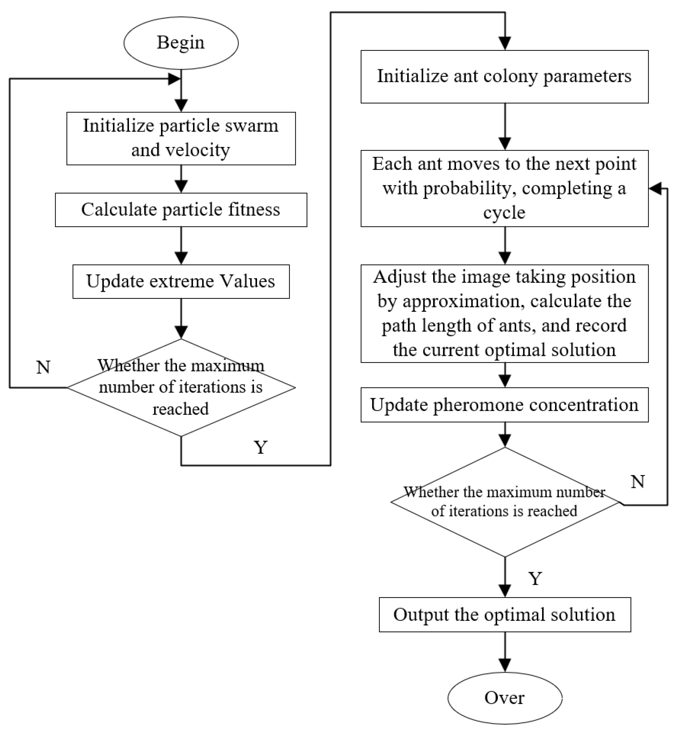
2.7.2. Improved Particle Swarm-Ant Colony Optimization Algorithm

IES planning and optimization models that consider uncertainty often must consider multiple aspects, including the economy, environmental friendliness, and reliability, and they are extremely complex to calculate. The traditional ant colony algorithm tends to fall into local optimal solutions, long computation time, and complicated adjustment parameters, which are not conducive to integrated energy system planning solutions. In this paper, an improved particle swarm-ant colony optimization algorithm is proposed, combining the advantages of the particle swarm with fewer parameters with the ant colony algorithm, considering the advantages of robustness of the ant colony algorithm, and improving the solution speed of the algorithm by reducing the number of algorithm parameters that need to be adjusted. The improved algorithm adopted in this paper can solve the defects of insufficient convergence of the optimization algorithm when facing multi-objective planning, easily calculate the cycle, and facilitate in finding the global optimal solution, and the specific parameters and steps are introduced as shown in

Table 1. Improved parameter setting for the particle swarm-ant colony optimization algorithm.

Name of the Parameter	Specific Values
$\mathrm{Maximum} \mathrm{particle} \mathrm{velocity} v_{\max }$	60
$\mathrm{Minimum} \mathrm{particle} \mathrm{velocity} v_{\min }$	20
Population size (number of individuals, number of dimensions)	40.10
$\mathrm{Acceleration} \mathrm{factor} c_1$	2
$\mathrm{Acceleration} \mathrm{factor} c_2$	2
Number of iterations	100
$\mathrm{Inertia} \mathrm{weights} \omega$	0.9
Number of ants	30
Heuristic factors	1.5
Expectation Heuristic Factor	5.0
Pheromone volatility factor	0.6
Pheromone intensity	350

below. Figure 4 shows the solution process of the improved particle swarm ant colony optimization algorithm.

Step 1: Initialize the position and velocity of the particle population.

Step 2: Calculate the fitness of each particle.

Step 3: Update the global best position. We compare the current adaptation value of each particle with the adaptation value corresponding to the global best position, and if the current adaptation value is higher, the global best position will be updated with the current particle’s position.

Step 4: Update the velocity and position of each particle according to the following formula:

$$v_{\mathrm{id}}^{\mathrm{k}}=w{v}_{\mathrm{id}}^{\mathrm{k}-1}+c_1{r}_1(pbes{t}_{id}-x_{id}^{k-1})+c_2{r}_2(gbes{t}_d-x_{id}^{k-1})$$

(32)

$$x_{id}^k=x_{id}^{k-1}+v_{id}^{k-1}$$

(33)

In the formula, $v_{id}^k$ is the $d$th dimensional component of the velocity vector of the $k$th iteration particle, $i$, flight. $x_{id}^k$ is the $d$th dimensional component of the position vector of the $k$th iteration particle, $i$. $c_1$ and $c_2$ are acceleration constants, which regulate the maximum learning step. $r_1$ and $r_2$ are two random functions, taking values in the range [0,1] to increase the search randomness. $w$ is the inertia weight, which is non-negative and regulates the search range of the solution space.

Step 5: Reach the maximum number of iterations to move to the next step, otherwise return to step 2.

Step 6: Initialization of the ant colony parameters and initialization of the pheromone matrix distribution of the ant colony algorithm using the suboptimal solutions obtained by the above algorithm.

Step 7: Pick a node at random, place the ant on it, calculate the probability value that it will shift, and find the next path.

Step 8: Update the pheromone concentration according to the following formula:

$${\tau }_i\left(t+1\right)=\{\begin{array}{c}\rho \cdot {\tau }_i\left(t\right)+\delta \left(t\right)if\left(x\in A\left(t+1\right)\right)\hfill \\ \rho \cdot {\tau }_i\left(t\right)\hspace{1em}\hspace{1em}\hspace{1em}\hspace{1em}\hspace{1em}\hspace{1em}\hspace{1em}else\end{array}$$

(34)

In the formula, $\delta \left(t\right)=\min \sqrt{{\displaystyle \sum _{i=1}^n\left(f_i\left(x\right)-f_i\left(x_v\right)\right)}}$, $x_v\in A\left(t\right)$, and $\rho$ is the volatilization factor.

Step 8: If the maximum number of cycles is reached, output the optimal solution; otherwise, return to step 7.

3. Results

3.1. Basic Data

In this paper, we took a park in the south as the planning object, and divided the year into three types of typical days according to the characteristics of clean energy output and customer-side behavior, namely summer, a transition season, and winter, with 91, 93, and 181 days for each season, respectively. The park consists mainly of commercial buildings, and the maximum electrical, cooling, and thermal loads in this area are 280 kW, 156 kW, and 344 kW, respectively. The time-sharing electricity prices in the region are shown in

Table 2. Time-sharing electricity price.

Time Period	Electricity Price
Peak hour (8–11, 18–23)	$0.23/kWh
flat load (11–18)	$0.11/kWh
Valley hour (23–7)	$0.09/kWh

below. In this paper, three typical days were selected, respectively, and the load forecast curves are shown in Figure 5 below.

3.2. Scenario Reduction Effectiveness Analysis

We generated many renewable energy output scenario by the scenario generation method, and then we repeated the reduction three times by different scenario reduction methods. The following table shows the comparison of some indicators when different reduction methods were used for scenario reduction, with 0–1 planning, an improved k-means clustering algorithm, and fast forward reduction, respectively, and the reduction results are shown in

Table 3. Scenario reduction results.

Reduction Method	Running Time/s	Euclidean Distance	Contour Factor
0–1 planning model	64.52	0.45	0.258
	78.84	0.69	0.011
	74.23	0.50	−0.263
Improved k-means clustering algorithm	12.45	0.11	0.623
	14.56	0.06	0.657
	10.55	0.07	0.642
Fast forward reduction	6.52	0.35	0.052
	5.98	0.41	0.019
	5.16	0.24	−0.235

below.

The k-means clustering algorithm proposed in this paper had the largest value of the contour coefficient index for three calculations, and the results were less different and tended to be stable, indicating that the method has a high and stable fitting accuracy, and the reduced scenarios could reflect the distribution characteristics of the original scenario set more accurately. Through the test of Euclidean distance, it was found that k-means clustering could make the cut scenarios maintain a high similarity with the initial scenarios. In terms of computational efficiency, the fast forward reduction method was the most computationally efficient, and the 0–1 planning model was the slowest to solve. Therefore, the improved k-means clustering algorithm is fully applicable to consider similar renewable energy output uncertainty problems in capacity planning.

4. Discussion

Under the condition of considering the uncertainty of the renewable energy output, the three load demands of electricity, heat, and cooling were satisfied, and the capacity of distributed energy equipment was planned. In order to highlight the innovation point of this paper, three scenarios were set for comparison with the base scenario to verify the effectiveness of the integrated energy system planning strategy, considering the scenery uncertainty proposed in this paper.

Base scenario: The scenario analysis method was not used, and the planning solution strategy proposed in this paper was not used.

Scenario 1: Instead of using the scenario analysis method, the planning solution strategy proposed in this paper was used.

Scenario 2: Using the scenario analysis method without using the planning solution strategy proposed in this paper.

Scenario 3: Using the scenario analysis method, while using the planning solution strategy proposed in this paper.

After solving the model constructed in this paper, the impact of the capacity planning scenarios obtained for the four scenarios on the economy and environmental friendliness of the integrated energy system is shown in

Table 4. Extent of economic impact on IES under different scenarios.

Scenario Type	Annualized Cost/$	Range of Change
Base scenario	293,820	0%
S1	270,263	Reduced by 8.02%
S2	243,695	Reduced by 17.06%
S3	226,585	Reduced by 22.89%

and

Table 5. Extent of environmental impact on IES under different scenarios.

Scenario Type	Carbon Emission/Kg	Range of Change
Base scenario	4266	0%
S1	3899	Reduced by 8.60%
S2	3803	Reduced by 10.85%
S3	3655	Reduced by 14.32%

below.

Analysis of the above data shows that Scenario 1, without considering the impact of uncertainty on system planning, reduced system costs and carbon intensity by a relatively small amount. For Scenario 2, after taking into account the uncertainty factor and adopting the scenario analysis method, although the planning solution strategy proposed in this paper was not used, the results obtained by the conventional solution also had obvious economic and environmental friendliness. Scenario 3 showed a significant reduction in annualized costs after using the scenario analysis method and the above solution strategy, fully demonstrating the effectiveness of the scenario reduction and planning solution strategy proposed in this paper. While ensuring it was economic, environmental friendliness was also improved. The carbon emissions of Scenario 3 dropped by 611kg of CO₂, which could play a role in low carbon emission reduction and meet the current development needs.

Table 6. Optimal solution equipment capacity and investment cost.

Equipment	Capacity/Kw	Investment Costs/$
PV	170	129,633
WT	780	593,561
Gas turbine	1200	61,730
Lithium bromide	1650	1,013,010
Ice storage	2650	395,707

below shows the optimal capacity planning scheme derived from Scenario 3.

The optimal planning scheme was put into operation to obtain the operating results of the integrated energy system, which is expressed as the equipment load situation for three typical days. According to the actual situation, in the summer and transition seasons, the thermal load demand was relatively small, and the heat energy generated by the gas turbine could fully bear the thermal load demand. However, the cold load demand was higher, and the cold load was borne by the electric cooler. In winter, the thermal load demand was relatively high, while the cold load demand was low, and the gas turbine generated relatively more power at this time, and the system’s power sales behavior was more significant. The histogram of purchased and sold power shows that the system usually bought power during low tariff hours for energy equipment consumption and used the gas turbine to generate more power during peak tariff hours to avoid buying power during high tariff hours with good economics.

In this paper, a typical summer day was selected as an example, and the typical equipment output and load data of the three subsystems of electricity, heat, and cooling are plotted as shown in Figure 6, Figure 7 and Figure 8 below.

As can be seen from Figure 6, in the summer, the main equipment output of the cold system had ice storage and melting, ice storage cooling (direct supply), and CCHP cold output, maintaining a higher power output during the day; from 22:00 to 7:00 the next day, the cold load was smaller, and the equipment output power was also reduced. Among them, from 8:00 to 18:00, the main equipment output was ice storage ice melt, and from 18:00 to 21:00 ice storage refrigeration started to replace ice melt output to supply the nighttime cold load, and the CCHP cold output was kept at a lower power throughout the day.

As can be seen from Figure 7, the main equipment output was a CCHP heat output, and it kept a low power operation throughout the day due to the low heat load demand in summer. In contrast to the cooling system load demand, the load and output power of the thermal system were relatively low from 8:00 to 21:00, with a small increase in the load and output power from 21:00 to 7:00 the following day.

As can be seen from Figure 8, the electrical system in summer had complex and large electrical loads for each equipment output datum. The lower CCHP electrical output during the all-day phase was mainly due to the fact that the gas turbine operates on heat-dependent power, and the heat demand was also low during the summer months, so the CCHP electrical output was kept low during the summer months. From 13:00 to 19:00, the system had electricity sales, mainly because the equipment load was low during this time, and the wind turbine and photovoltaic generation was sufficient to meet the internal consumption of the system and generate excess electricity that could be sold, which has good economic benefits. The rest of the time, the system mainly purchased power to meet various load demands.

Below is a comparison between the algorithm taken in this paper and Tabu Search (TS), Simulated Annealing (SA), Genetic Algorithm (GA), Particle Swarm Optimization (PSO), and Ant Colony Optimization (ACO).

(1)

Analysis of convergence characteristics

In this paper, we set the number of genetic generations to 100 and the population size to 1000, and we compared the changes in the iterative convergence curves of the six algorithms. Figure 9 shows iterative curves for different algorithms as they perform the solution calculations.

The graph above shows the convergence of the six algorithms with a population size of 1000. As can be seen from the graph, the improved Particle Swarm-Ant Colony Optimization algorithm (PSO-ACO) had a stronger convergence, and PSO performance was in the middle to upper level, while the GA had the weakest convergence-seeking performance. In the order of convergence of the above six algorithms from strong to weak, it was PSO-ACO, SA, PSO, TS ACO, and GA.

(2)

Solving for speed

The figure above shows the comparison of the solution speed of different algorithms for different population sizes. As can be seen from the figure, the convergence time to reach the optimal solution for all six algorithms increased as the population size increased. PSO-ACO had the lowest combined convergence time and therefore exhibited the best iterative performance among the six algorithms. The six algorithms ranked from fastest to slowest in terms of solution speed are PSO-ACO, GA, ACO, SA, TS, and PSO. Figure 10 shows the comparison of convergence times of different algorithms.

(3)

Accuracy of the solution algorithm

From the optimal solutions of the six algorithms, it can be seen that the PSO-ACO had the lowest total annual cost of $1,275,127, with the best accuracy; followed by PSO with $1,344,930; the ACO in third place with $1,476,938; and the SA and the TS with $1,675,424 and $1,760,897, respectively, while the GA had the highest total annual cost of $2,297,002, with the worst accuracy.

Table 7. Optimal solution for the total annual cost of different algorithms under planning scenarios.

Type of Algorithm	Optimum Annual Total Cost/$
TS	1,760,897
SA	1,675,424
GA	2,297,002
PSO	1,344,930
ACO	1,476,938
PSO-ACO	1,275,127

shows the optimal solution for the total annual cost of different algorithms under planning scenarios.

By comparing the solution accuracy, solution speed, and convergence characteristics of the six types of algorithms in this planning scenario, the improved particle swarm ant colony algorithm had a good performance, so the improved particle swarm ant colony algorithm was selected as the final planning solution algorithm in this paper.

5. Conclusions

In this paper, a scenario analysis was used to generate and reduce the uncertainty scenarios of scenery output and to simulate the planning of an integrated energy system in a park in southern China.

(1)

Scenario reduction was performed by an improved k-means clustering algorithm, by comparing it with the 0–1 planning method and the fast forward reduction method. The k-means clustering algorithm selected for this paper had a contour coefficient metric value of 0.67 and an improvement of approximately 254%. The Euclidean distance test metric value was 0.06, with a reduction of approximately 400%. The run time was 10.55 s, which is one-sixth of the original time compared to the 0–1 planning method, and the reduced scenarios maintained a high degree of similarity to the initial scenarios and accurately represent the distribution of the original set of scenarios.

(2)

The equipment planning capacity configuration after solving in this paper is PV 164kW, WT 750 kW, gas turbine 1300 kW, lithium bromide 1600 kW, and ice storage 2500 kW, and the optimal planning scheme was put into operation to obtain the operation results of the integrated energy system, and the corresponding output curve was drawn, which could reliably meet the needs of various types of loads throughout the planning cycle.

(3)

Compared with the original plan, the planned and optimized configuration plan reduced the annualized cost by $42,705 and carbon dioxide emissions by 521 kg. While considering the overall economy, it also took into account the overall environmental protection of the system.

The model constructed in this paper effectively solved the situation where the scenery output within an integrated energy system is highly volatile and uncertain, making it difficult to plan the system accurately, and it significantly reduced the cost and CO₂ emissions of integrated energy system planning and optimization when considering uncertainty. However, there are still many directions that can be expanded on the basis of this paper. On the one hand, only economic and environmental indicators were considered in this paper, but in the future, various indicators such as energy utilization can be added to the objective function. On the other hand, this paper only took into account the stochastic power output on the power side but not the uncertainty on the load side, which could be taken into account in future research to achieve more accurate planning.