Assessment of Forest Wood and Carbon Stock at the Stand Level: First Results of a Modeling Approach for an Italian Case Study Area of the Central Alps

Abstract

Models for carbon (C) stock assessment are widely applied in forest science, and mainly differ according to the scale of application, the required data, and the objectives for their implementation. This work presents the methodology implemented into the second version of an empirical model, WOody biomass and Carbon ASsessment (WOCAS v2), that uses the data of forest management plans (FMP) to calculate the mass of wood (t∙year⁻¹ of dry matter, DM) and C (t∙year⁻¹ C) at the stand level and from the year in which the FMPs came into force until a predefined reference year, for an Italian Case Study Area of Central Alps. The mass of wood and C are computed for (i) aboveground wood biomass (AWB), (ii) belowground wood biomass (BWB), and (iii) dead organic matter (DOM; i.e., dead wood and litter) according to the 2006 IPCC Guidelines. WOCAS v2 was tested for the first time for 2019 public forest stands (3.67 × 10⁴ ha) of Valle Camonica for the period 1984–2018. Results showed that, in 2018 and at the landscape level, the total living wood biomass (TLB; AWB + BWB) reached 5.35∙10⁶ t DM. TLB yield (t·ha⁻¹·year⁻¹ DM) ranged from 44.72 ± 44.42 t·ha⁻¹·year⁻¹ DM (1984) to 145.49 ± 70.76 t·ha⁻¹·year⁻¹ DM (2018). In the same year, DOM amounted to 6.12∙10⁵ t DM, ranging from 8.28 ± 7.79 t·ha⁻¹·year⁻¹ DM (1989) to 17.11 ± 12.03 t·ha⁻¹·year⁻¹ DM (2015). The total weighted C yield, computed as the sum of C yield in AWB, BWB, and DOM of each stand, ranged from 26.63 ± 26.80 t∙ha⁻¹∙year⁻¹ C (1984) to 80.28 ± 41.32 t∙ha⁻¹∙year⁻¹ C (2018). The results demonstrated that FMPs data can be useful in estimating wood and C mass at the stand level and their variation over space and time for AWB as well as for BWB and DOM, which are not considered in the FMPs. This can represent a starting point for defining sustainable forest management policies and practices to improve forest vitality and conservation in compatibility with ecosystem services provision. Moreover, as the model is based on a standardized methodology it can be applied in any other forest area where the same input data are made available; this may constitute the basis for further applications on a broader scale.

1. Introduction

In Europe, forests cover approximately 2.27 × 10⁸ ha (34.8% of the total area), which represents about 5% of the world’s forest area. About 87% of European forests is classified as semi-natural, 4% as natural, and 9% as plantations. Over hundreds of years, climatic conditions and environmental and hydrological factors together with human practices have promoted the establishment of several types of forests characterized by different management systems, functions, and species [1].

The role of forests has received increased attention in the context of global warming and climate change mitigation through the United Nations Framework Convention on Climate Change (UNFCCC, 1992) [2] and the Kyoto Protocol, and was recently further emphasized through the Paris Agreement (November 2016) and the EU regulation 2018/841 for the Land Use, Land Use Change and Forestry (LULUCF) Sector [3].

Forests remove atmospheric CO₂, resulting in its accumulation in both aboveground and belowground biomass; a fraction of this C is then transferred to the deadwood, litter, and soil due to natural mortality (self-thinning due to senescence and competition for light, water, and nutrients), natural disturbances, and logging residues (e.g., branches, tops, noncommercial wood parts, and small stems which fall into the ground during harvesting) that remain at the felling site once roundwood is collected. At the same time, mortality, wood collection, and decomposition processes can cause re-emission of this sequestered C directly into the atmosphere [4,5,6,7].

The mass of the stored C (i.e., C stock) depends on the mass of wood and its dynamics, and can therefore increase or decrease according to environmental conditions, forest structure (e.g., tree density, species, and age), silvicultural treatments, and mortality. Therefore, by computing the trend of C mass over a given period it is possible to evaluate whether forests act as C sinks or sources in order to assess their role in mitigating climate change [1,8].

Models for C stock assessment are widely applied, and mainly differ according to their scale of application, required input data, and output results, and are generally classified as either mechanistic or empirical [9,10].

Mechanistic models simulate the growth of a forest by considering the interaction among the physiological processes on which the growth itself is based, i.e., photosynthesis, respiration, and allocation of photosynthates to leaves, stems, and roots [9,10,11]. These models generally require complex input data/information which are not always made available from forest inventory or local forest plans, causing difficulties in their use [9]. Moreover, the output results (e.g., gross or net primary production) are not always of interest or practical help for forest management [9,12].

On the other hand, empirical models describe a forest’s development through regression equations that are parameterized using extensive datasets, excluding the processes that control forest growth from a physiological point of view, and are generally classified into single-tree, size-class, and whole-stand models.

In single-tree models, in which the basic unit of modeling is the tree, input data such as tree dimensions, tree height, and crown characteristics are used to provide detailed information about the growth of different tree compartments and their characteristics [13]. Single-tree models can in turn be either distance-dependent, which requires the location of each tree and the distance among trees as input data, or distance-independent, in which case it is assumed that trees are randomly distributed. Examples of single-tree models include TASS [14], PROGNAUS [15], SILVA [16], and FVS [17].

Size-class models provide information on the forest’s structure and as an output result generally produce a histogram displaying the distribution of stem diameters. This type of model represents a compromise between whole-stand and single-tree models; when the class size is large and only one diameter class exists, the model can be considered as a whole-stand model, while when different diameter classes exist, the model is considered a single-tree model [9,10]. Examples of size-class models include FIBER [18] and CAFOGROM [19].

In whole-stand models, the basic unit of modeling is the stand, defined as a group of trees over a specific area and sufficiently uniform in terms of species, structure, management practices, and soil conditions to be distinguished from other tree groups in neighboring areas. Each stand is classified according to a few attributes such as stem volume, basal area, or tree density, and the change in these attributes over time is simulated. Widely used whole-stand models include DFSIM [20], TADAM [21], and GNY [22]. Even if these models are the simplest empirical ones, they are widely adopted in forest management [9] because they are suitable for evaluating the impact of different silvicultural treatments on forest C stock over time [23,24]. Nevertheless, they generally do not consider the impact of climate change [9] and variation in soil productivity due to nitrogen deposition and atmospheric CO₂ concentration [25]; therefore, future projections should be limited to the short period of time for which it is reasonable to assume that growth and C stock are mainly affected by forest structure and silvicultural treatments and over which natural disturbances do not occur [26].

Empirical models are currently applied at both continental [27], national [28,29], regional [30,31], and local [26] scales. This latter level of analysis is particularly important for Italy, where the main tool to manage public forests is the forest management plan (FMP). A generic FMP is based on the single forest stand as its management unit and defines for a given stand the silvicultural treatments to be carried out over a specific period of time to increase the productive, environmental, naturalistic, and social functions of the forest [32]. Each FMP has a duration between 10 and 15 years and is generally prepared by local forestry authorities such as mountain communities, i.e., local bodies that connect municipalities of alpine and pre-alpine areas and are aimed at improving the socioeconomic conditions of mountainous landscapes [33]. FMPs provide several types of data and information that are often neglected which, if properly managed, can be used to estimate forest wood and C stock at different space and time scales [34]. For this purpose, the main piece of quantitative data that is always made available is the total merchantable stem volume, i.e., the volume of the stem that can be used for commercial purposes, whereas more specific information such as tree number and the corresponding volume, or average tree diameter, are not always reported. Under these conditions, using whole-stand models for biomass and C stock estimation is the only feasible solution.

In addition to C sequestration, forests contribute to climate change mitigation by making wood available for energy generation [35,36,37,38,39] or long life-cycle products such as furniture, doors, flooring, or packaging [40,41]. Therefore, local decision-makers can be supported in forest management by providing them with models aimed at the quantification of forest biomass and C stock on the one hand, and wood for building and energy purposes on the other.

To achieve this specific goal, the first version of the empirical stand-level model WOody biomass and Carbon Assessment (WOCAS v1) [42] was improved in establishing the second version (WOCAS v2), which is described here. In WOCAS v1, a retrospective analysis (i.e., for each stand, from the year in which the FMP entries into force until a predefined reference year) is performed, and the mass of C (t·year⁻¹ C) is computed in (i) aboveground wood biomass (AWB), (ii) belowground wood biomass (BWB), (iii) deadwood, and (iv) litter. Starting from this point, the model provides the possibility of analyzing future scenarios based on the continuation of the current management practices or the adoption of improved ones (e.g., conversion of abandoned coppices to high forests) in order to define a possible mitigation strategy at the local level for the activation of Voluntary Carbon Markets.

Compared to WOCAS v1, WOCAS v2 is specifically focused on retrospective analysis, and it provides a more comprehensive assessment of the mass of wood and C at the stand level; the transfer of wood and C within the forest pools are simulated for each analyzed year according to biomass increment, losses to due self-thinning, natural disturbances, wood collection, and dead organic matter (DOM; i.e., dead wood and litter) decomposition. Therefore, unlike other models and approaches in which the calculations are performed starting from data made available by regional/national forest inventories and often only for the AWB, WOCAS uses data from FMPs and performs the calculations for different ecosystem pools. In detail, compared to the previous version the main improvements of WOCAS v2 are: (i) calculation of the gross annual increment of each stand through an age-independent nonlinear growth function based on the merchantable stem mass; (ii) estimation of the AWB using biomass expansion factors alternately defined for each classification criteria code (see Section 2) or for each stand; (iii) inclusion of self-thinning and natural disturbances in the simulation; (iv) quantification of the mass of wood and C in the DOM according to the annual inputs (self-thinning, natural disturbances, producible logging residues) and output (decomposition); and (v) calculation of the mass of C within each pool for each year of analysis.

In addition to wood and C mass assessment, a methodology was implemented into WOCAS v2 to calculate the mass of logging residues (branches and tops only; t·year⁻¹ DM) potentially available for energy generation. This is another important and innovative aspect which distinguishes WOCAS v2 from WOCAS v1 and other models, as extraction of logging residues is not always considered even if it plays a crucial role in defining C balance at the stand level. The methodology for residues estimation has already been presented in [38] and is not covered here; therefore, when applying WOCAS v2 to the Case Study Area, it was assumed that all the producible logging residues were left inside the stand after stem collection.

Considering all these elements, the aims of the current work are: (i) to present the methodology implemented into WOCAS v2 for the quantification of the mass of wood and C for AWB, BWB, and DOM for a generic forest stand; and (ii) to present the results derived from the first application of the improved methodology to 2019 public forest stands of Valle Camonica (Lombardy region, Italy), covering the period 1984–2018.

Valle Camonica was selected as a representative Case Study in Northern Italy as it is one of the biggest valleys of the Central Alps and is characterized by an extensive forest area (i.e., 3.67 × 10⁴ ha) covered by 45 FMPs; this makes the use of FMP data particularly interesting for wood and C mass estimation. The north-eastern part of the valley is covered by the Adamello Regional Park, which includes a Special Protection Area (ZPS) and fifteen Sites of Community Importance (SCI); in this context, forests are managed by applying a multifunctional approach [8] to balance their ecological, economic, and social functions while at the same time considering society’s needs. For this purpose, the results of this study can represent a starting point to address policies and practices aimed at improving forest vitality and conservation in a way compatible with C stock and other ecosystem services.

Finally, the values of C stock resulting from this analysis can be firstly compared to those obtained through the previous version of the model to evaluate how the new version improves the results, and with others commonly available in the literature for local, national, and international scales in order to better assess the contribution of Valle Camonica forests in stocking C for climate change mitigation.

2. Materials and Methods

Similar to the first version of the model [42], in WOCAS v2 the wood and C stock is calculated through two spreadsheets (MS Office Excel^®) for parameter selection and C storage assessment. In the first, a generic stand “j” is classified according to three sub-criteria (SC):

• SC₁—forest structure
• SC₂—forest function
• SC₃—forest typology and variants

Each SC is associated with a sub-code, and the combination of sub-codes produces a classification criteria code (CCC) to which specific parameters are linked and uploaded into the second spreadsheet. Figure 1 shows the general framework for parameter selection; for further details, see [42] and the Supplementary Materials. The second spreadsheet is made up of a database in which each stand represents a record organized in different fields containing the specific input data and output results. To increase the flexibility of the model, control fields provide the possibility, through a selection at the beginning of each record, of resetting all the fields related to a specific stand, excluding it from the analysis. The wood and C stock is computed for each “j” stand and for each year “n” through a mass balance based on a “gain–loss” approach in AWB, BWB, and DOM (

Table 1. Definition of the pools considered by WOCAS v2 (modified from [31,43]).

N.	Name	Definition
1	Aboveground wood biomass (AWB)	Over-bark living wood biomass above the soil surface related to stems and branches of all dimensions; foliage is excluded.
2	Belowground wood biomass (BWB)	Living wood biomass of coarse live roots (diameter D ≥ 2 mm); fine roots (D < 2 mm) are included in the soil organic matter or litter as they cannot be empirically distinguished.
3	Dead organic matter (DOM)	Deadwood includes all nonliving wood biomass not contained in the litter, both standing and lying on the soil surface, with D ≥ 10 cm.
		Litter includes all nonliving wood biomass with D < 10 cm, including wood under different stages of decomposition above the mineral or organic soil, and fine roots.

).

For each j-stand, the following input data are required:

• starting (YR_S(j)) and deadline (YR_D(j)) year of the FMP
• forest structure
• forest function
• forest typology and variants
• forest area (A_(j); ha)
• merchantable stem volume at YR_S(j) (MV_YRs(j); m³·year⁻¹)
• gross annual increment of the merchantable stem volume at YR_S(j) (GAI_YRs(j); m³·year⁻¹)
• harvested merchantable stem volume for each year n (MV_Hn(j); m³·year⁻¹)

Before the simulations, volume values are converted into mass values through the parameter k₁ (wood basic density, ratio between wood DM and wood fresh volume; t∙m⁻³ DM). Figure 2 shows the general approach on which WOCAS v2 is based.

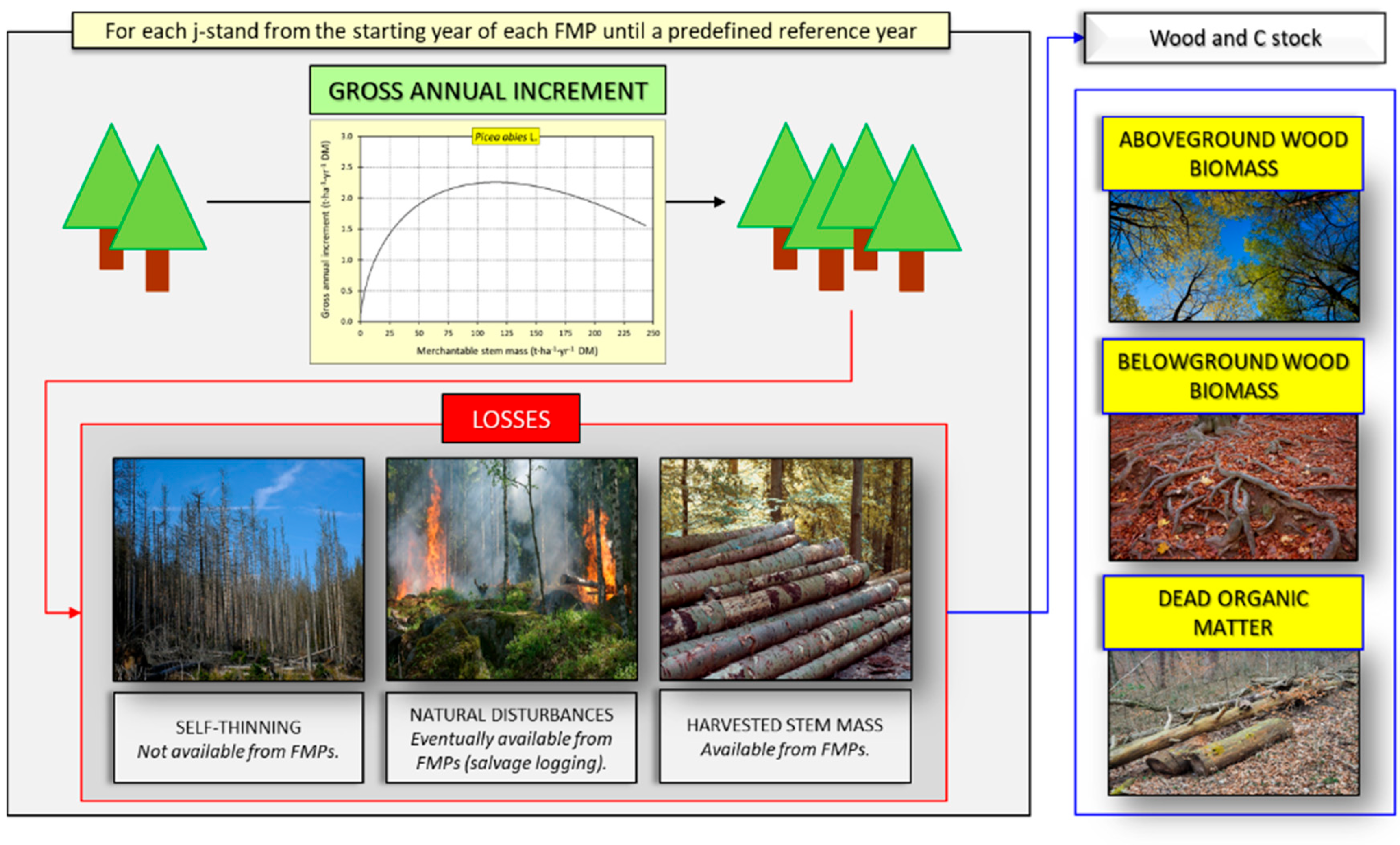
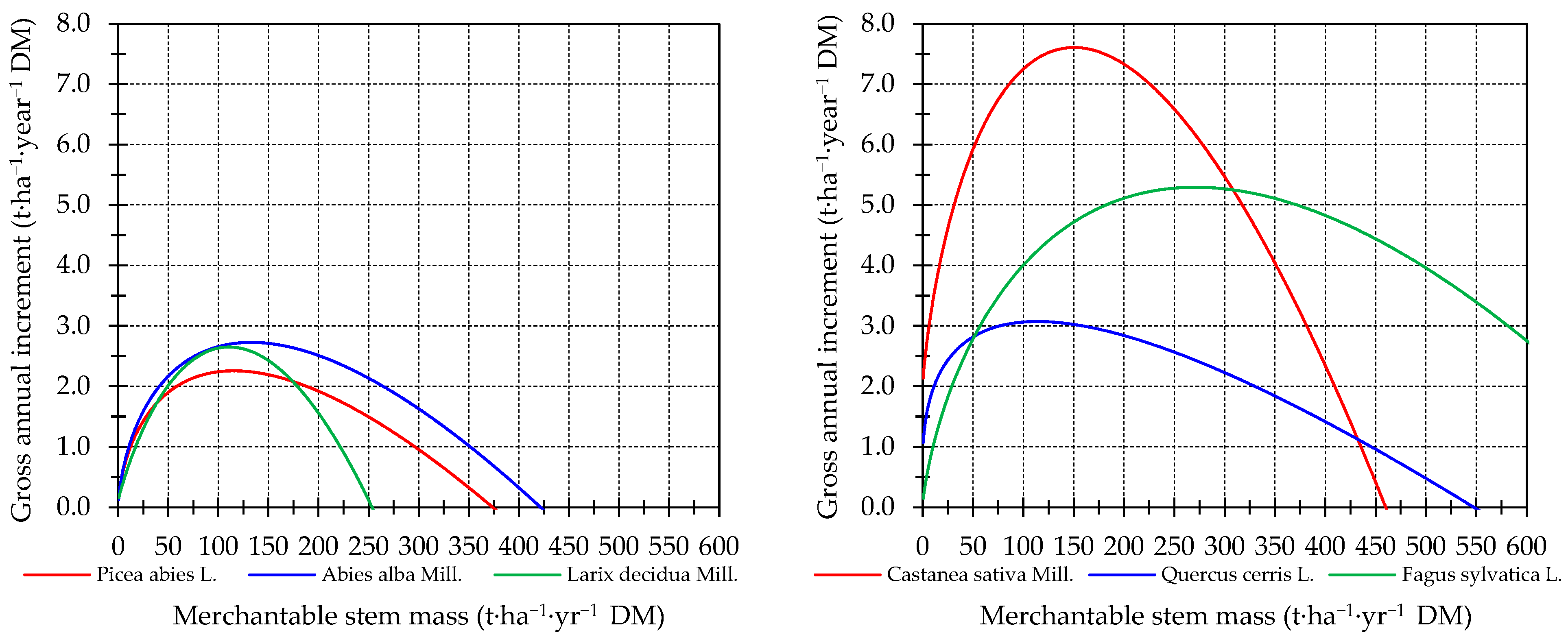
2.1. Gross Annual Increment

While in WOCAS v1 calculations are performed by using the gross annual increment provided by the FMPs at YR_S(j) (which is assumed as constant over time) for each j-stand and for each year n, in WOCAS v2 the user has to choose whether to use a constant or variable gross annual increment (GAI_n(j); t∙year⁻¹ DM). In this last case, for each j-stand and for each year n the increment is computed through the first derivative of the mass with respect to time of the theoretical function of Richards [44], which is expressed as [31,45,46]:

$${\mathrm{MM}}_{\mathrm{n}\left(\mathrm{j}\right)}^{*}={\mathrm{k}}_2·{\left[1-{\mathrm{e}}^{\left({\mathrm{k}}_3-{\mathrm{k}}_4·\mathrm{t}\right)}\right]}^{-1/{\mathrm{k}}_5}$$

(1)

where:

• ${\mathrm{MM}}_{\mathrm{n}\left(\mathrm{j}\right)}^{*}$: merchantable stem mass at the beginning of the year n per unit of area (t·ha⁻¹∙year⁻¹ DM);
• k₂: maximum value of ${\mathrm{MM}}_{\mathrm{n}\left(\mathrm{j}\right)}^{*}$, i.e., carrying capacity (t·ha⁻¹·year⁻¹ DM; k₂ > 0);
• e: Euler’s number (constant equal to 2.718);
• k₃: growth parameter which allows the time at which ${\mathrm{MM}}_{\mathrm{n}\left(\mathrm{j}\right)}^{*}$ = k₂/2 to be varied (dimensionless);
• k₄: relative growth rate, i.e., rate of accumulation of new DM per unit of existing DM (year⁻¹; k₄ > 0);
• t: time (years); and
• k₅: shape parameter which allows the curve inflexion point to be at any value between the minimum and the maximum of ${\mathrm{MM}}_{\mathrm{n}\left(\mathrm{j}\right)}^{*}$ (dimensionless; −1 ≤ k₅ ≤ + ∞; k₅ ≠ 0).

The Richards function is expressed as a nonlinear regression curve with a sigmoid trend and represents a generalization of other widely used functions, such as the exponential (k₂ → + ∞; k₅ > 0), the logistic (k₅ > 1), the Bertalanffy (k₅ = 3), and the Gompertz (k₅ → ± ∞). This function allows simulating asymmetrical “patterns” of growth in which the maximum value of the gross annual increment can be reached at any value of the merchantable mass between 0 and the carrying capacity; from a biological point of view, it expresses the net photosynthesis (i.e., the difference between gross photosynthesis and respiration) [31,47,48]. The first derivative of Equation (1) is:

$${\mathrm{GAI}}_{\mathrm{n}\left(\mathrm{j}\right)}=\left[\frac{{\mathrm{k}}_4}{{\mathrm{k}}_5}·{\mathrm{MM}}_{\mathrm{n}\left(\mathrm{j}\right)}^{*}·\left[1-{\left(\frac{{\mathrm{MM}}_{\mathrm{n}\left(\mathrm{j}\right)}^{*}}{{\mathrm{k}}_2}\right)}^{{\mathrm{k}}_5}\right]+{\mathrm{k}}_6\right]·{\mathrm{A}}_{\left(\mathrm{j}\right)}$$

(2)

where:

• A_(j): forest area of the j-stand (ha);
• k₆: increment of the stand at the age of 1 year; this parameter does not derive from the calculation of the first derivative itself, rather, it is required to define the starting point of the function (t·ha⁻¹·year⁻¹ DM; k₆ > 0).

Through Equation (2), the gross annual increment of a given year is directly linked to the merchantable mass at the beginning of the same year; in particular, the increment increases as the merchantable mass increases from low values, reaches a maximum at the point of inflection and then decreases toward zero when the mass reaches the carrying capacity.

As an example, Figure 3 shows the trend of the gross annual increment for three coniferous (Picea abies L., Abies alba Mill., and Larix decidua Mill.) and for three broadleaved (Castanea sativa Mill.—management system: coppice; Quercus cerris L.—management system: high forest; Fagus sylvatica L.—management system: high forest) species computed by using specific values for growth parameters derived from the literature and calibrated for the Lombardy region according to the data made available in the regional yield tables [46]. Figure 4 shows, for the same species and management systems, the trend of the gross merchantable stem mass over time.

For further details regarding the values of the parameters for all the species and management systems of this study, refer to the Supplementary Materials.

Once GAI_n(j) is computed, WOCAS v2 calculates the mass of wood in the AWB, BWB, and DOM by taking into account the net annual increment and the harvested merchantable stem mass; finally, the mass of C in each pool is quantified.

2.2. Net Annual Increment

The net annual increment (NAI_n(j); t·year⁻¹ DM), not considered in the previous model version, is here computed as [13,49]:

$${\mathrm{NAI}}_{\mathrm{n}\left(\mathrm{j}\right)}={\mathrm{GAI}}_{\mathrm{n}\left(\mathrm{j}\right)}-{\mathrm{MM}}_{\mathrm{Sn}\left(\mathrm{j}\right)}-{\mathrm{MM}}_{\mathrm{Dn}\left(\mathrm{j}\right)}$$

(3)

where MM_Sn(j) and MM_Dn(j) represent the losses of merchantable stem mass (t·year⁻¹ DM) due to self-thinning and natural disturbances, respectively.

Losses due to self-thinning generally occur each year and can reach 30–50% of GAI_n(j) in natural stands without periodic wood cuts, whereas they can be negligible in regularly managed stands as cuts generally remove wood that otherwise would be transferred to the DOM [43]. If expressed as a fraction of the stem mass self-thinning can reach 1.2% of the mass, with some differences between coniferous and broadleaved species [50].

To increase the flexibility of WOCAS v2, the user must choose, for each classification criteria code, whether to express MM_Sn(j) as a fraction of the stem mass (0–1.2%) or of GAI_n(j) (0–50%); in both cases, it is possible to choose whether to use the average value or any other one between the minimum and maximum defined by the model.

For natural disturbances, the user must define (i) year of occurrence, (ii) targeted volume (m³·year⁻¹), and (iii) type (1—wildfire; 2—windstorm; 3—insect outbreak; 4—other).

2.3. Harvested Merchantable Stem Mass and Potentially Producible Logging Residues

For each j-stand and for each year n in which wood cuts occurred, the harvested merchantable stem mass (MM_Hn(j); t·year⁻¹ DM) is quantified, as in WOCAS v1, according to MV_Hn(j); (m³·year⁻¹) and the parameter k₁. On the other hand, the mass of the potentially producible logging residues (RP_n(j); t·year⁻¹ DM), not accounted for in the previous model version, is here computed as [43]:

$${\mathrm{RP}}_{\mathrm{n}\left(\mathrm{j}\right)}=({\mathrm{MM}}_{\mathrm{Hn}\left(\mathrm{j}\right)}·{\mathrm{k}}_7)-{\mathrm{MM}}_{\mathrm{Hn}\left(\mathrm{j}\right)}$$

(4)

where the parameter k₇ expresses the biomass expansion factor, defined as the total aboveground wood volume on the merchantable stem volume. Similarly, under the assumption that k₁ does not change between stem and branches, k₇ can expresses the total aboveground wood biomass DM on the merchantable stem mass DM.

2.4. Aboveground and Belowground Wood Biomass

The merchantable stem mass at the end of a given year (MM_n(j); t·year⁻¹ DM) is

$${\mathrm{MM}}_{\mathrm{n}\left(\mathrm{j}\right)}={\mathrm{MM}}_{\mathrm{n}-1\left(\mathrm{j}\right)}+{\mathrm{NAI}}_{\mathrm{n}\left(\mathrm{j}\right)}-{\mathrm{MM}}_{\mathrm{Hn}\left(\mathrm{j}\right)}$$

(5)

where MM_n−1(j) is the merchantable stem mass at the end of the year n − 1 (t·year⁻¹ DM).

Finally, the aboveground and belowground wood biomass DM (AWB_n(j), BWB_n(j), respectively; t·year⁻¹ DM) are

$${\mathrm{AWB}}_{\mathrm{n}\left(\mathrm{j}\right)}={\mathrm{MM}}_{\mathrm{n}\left(\mathrm{j}\right)}·{\mathrm{k}}_7$$

(6)

$${\mathrm{BWB}}_{\mathrm{n}\left(\mathrm{j}\right)}={\mathrm{MM}}_{\mathrm{n}\left(\mathrm{j}\right)}·{\mathrm{k}}_8$$

(7)

where k₈ is the root-to-shoot ratio, i.e., belowground coarse root mass DM on merchantable mass DM.

The total living wood biomass is

$${\mathrm{TLB}}_{\mathrm{n}\left(\mathrm{j}\right)}={\mathrm{AWB}}_{\mathrm{n}\left(\mathrm{j}\right)}+{\mathrm{BWB}}_{\mathrm{n}\left(\mathrm{j}\right)}$$

(8)

Calculations performed through Equations (5)–(8) are common to both model versions, except for Equation (5) in which the constant FMP gross annual increment is used instead of the net one.

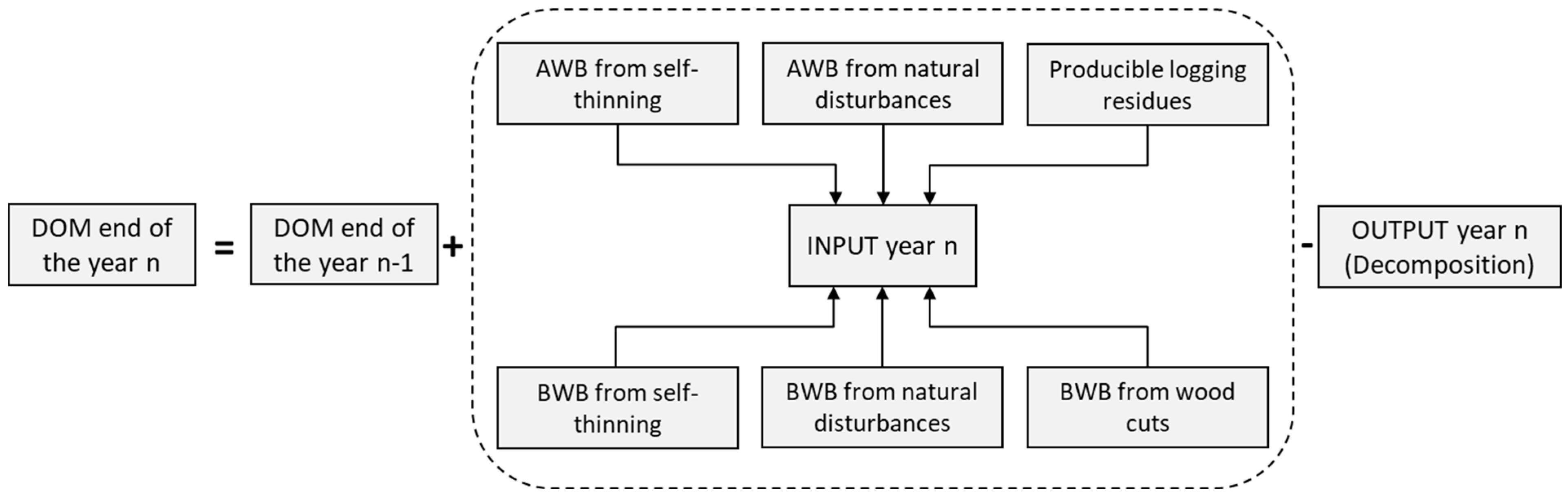
2.5. Dead Organic Matter

In WOCAS v1 the mass of deadwood and litter is computed separately in a simplified way, as a function of the AWB through linear equations (i.e., the higher the AWB, the higher the deadwood and litter, and vice versa) applied at the regional level for C stock accounting within the UNFCCC.

In the improved version the mass of deadwood and litter is computed as a whole as DOM by applying a specific mass balance according to annual inputs and outputs [43]:

$${\mathrm{DOM}}_{\mathrm{n}\left(\mathrm{j}\right)}={\mathrm{DOM}}_{\mathrm{n}-1\left(\mathrm{j}\right)}+{\mathrm{DOM}}_{\mathrm{INn}\left(\mathrm{j}\right)}-{\mathrm{DOM}}_{\mathrm{OUTn}\left(\mathrm{j}\right)}$$

(9)

where:

• DOM_n(j): mass of wood in the DOM at the end of the year n (t∙year⁻¹ DM);
• DOM_n−1(j): mass of wood in the DOM at the end of the year n − 1 (t∙year⁻¹ DM);
• DOM_INn(j): DOM inputs in the year n (t∙year⁻¹ DM); and
• DOM_OUTn(j): DOM outputs in the year n (t∙year⁻¹ DM).

Only for the starting year of the simulation, the initial value of DOM (DOM_YRs(j), which is equal to DOM_n−1(j); t∙year⁻¹ DM), is

$${\mathrm{DOM}}_{\mathrm{YRs}\left(\mathrm{j}\right)}={\mathrm{MM}}_{\mathrm{YRs}\left(\mathrm{j}\right)}·{\mathrm{k}}_7·{\mathrm{k}}_9$$

(10)

where:

• MM_YRs(j): merchantable stem mass at the starting year of the FMP (t∙year⁻¹ DM);
• k₉: deadwood expansion factor (deadwood DM on aboveground wood biomass DM).

DOM_INn(j) (t∙year⁻¹ DM) is:

$${\mathrm{DOM}}_{\mathrm{INn}\left(\mathrm{j}\right)}=({\mathrm{MM}}_{\mathrm{Sn}\left(\mathrm{j}\right)}·{\mathrm{k}}_7)+({\mathrm{MM}}_{\mathrm{Sn}\left(\mathrm{j}\right)}·{\mathrm{k}}_8)+({\mathrm{MM}}_{\mathrm{Dn}\left(\mathrm{j}\right)}·{\mathrm{k}}_7·{\mathrm{k}}_{10})+({\mathrm{MM}}_{\mathrm{Dn}\left(\mathrm{j}\right)}·{\mathrm{k}}_8)+{\mathrm{RP}}_{\mathrm{n}\left(\mathrm{j}\right)}+({\mathrm{MM}}_{\mathrm{Hn}\left(\mathrm{j}\right)}·{\mathrm{k}}_8)$$

(11)

where

• MM_Sn(j) k₇: aboveground biomass transferred to the DOM due to self-thinning (t∙year⁻¹ DM);
• MM_Sn(j) k₈: belowground biomass transferred to the DOM due to self-thinning (t∙year⁻¹ DM);
• MM_Dn(j) k₇ k₁₀: aboveground wood biomass transferred to the DOM due to natural disturbances (t∙year⁻¹ DM); k₁₀ (−) is the fraction of aboveground wood biomass which is transferred to the DOM according to the type of disturbance. For wildfire, a value of k₁₀ = 0.5 is adopted [51] as a default under the hypothesis that 50% of the targeted aboveground wood biomass is transferred to the DOM and the other fraction is lost through the atmosphere. For all the other types of disturbance, k₁₀ = 1.0, i.e., 100% of the targeted biomass is transferred to the DOM.
• MM_Dn(j) k₈: belowground biomass transferred to the DOM due to natural disturbances (t∙year⁻¹ DM);
• RP_n(j): potentially producible logging residues (t∙year⁻¹ DM); and
• MM_Hn(j) k₈: belowground wood biomass transferred to DOM due to wood cuts (t∙year⁻¹ DM).

DOM_OUTn(j) (t∙year⁻¹ DM) refers to the decomposition, and is estimated as

$${\mathrm{DOM}}_{\mathrm{OUTn}\left(\mathrm{j}\right)}=({\mathrm{DOM}}_{\mathrm{n}-1\left(\mathrm{j}\right)}+{\mathrm{DOM}}_{\mathrm{INn}\left(\mathrm{j}\right)})·{\mathrm{k}}_{11}$$

(12)

where k₁₁ is the DOM decomposition rate (year⁻¹).

In all cases in which the parameter k₇ is used, while in WOCAS v1 simulations are performed by using average constant values for each classification criteria code, in WOCAS v2, as already reported in [38], the user can perform the simulations by using constant values for each j-stand. Even if in both cases the values of k₇ are defined at the beginning of the simulation and are assumed as constant over time, in the first case the same value of k₇ is associated with stands with the same classification criteria code, whereas in the second case the value of k₇ is specifically estimated for each j-stand through a non-linear regression equation [52] which expresses the tendency of branchiness as a function of the stem mass:

$${\mathrm{k}}_{7\left(\mathrm{j}\right)}={\mathrm{k}}_{12}+{\mathrm{k}}_{13}/{\mathrm{MM}}_{\mathrm{YRs}\left(\mathrm{j}\right)}^{*}$$

(13)

where:

• ${\mathrm{MM}}_{\mathrm{YRs}\left(\mathrm{j}\right)}^{*}$: merchantable stem mass per unit of area at the starting year of the FMP (t∙ha⁻¹∙year⁻¹ DM); and
• k₁₂, k₁₃: parameters for each classification criteria code (k₁₂: dimensionless; k₁₃: t∙ha⁻¹ DM).

Figure 5 shows the logical framework implemented into WOCAS v2 for estimating the DOM mass.

2.6. Carbon Mass

The mass of C in (i) AWB, (ii) BWB, and (iii) DOM (C_AWBn(j), C_BWBn(j), and C_DOMn(j), respectively, in t·year⁻¹ C) is

$${\mathrm{C}}_{\mathrm{AWBn}\left(\mathrm{j}\right)}={\mathrm{AWB}}_{\mathrm{n}\left(\mathrm{j}\right)}·{\mathrm{k}}_{14}$$

(14)

$${\mathrm{C}}_{\mathrm{BWBn}\left(\mathrm{j}\right)}={\mathrm{BWB}}_{\mathrm{n}\left(\mathrm{j}\right)}·{\mathrm{k}}_{15}$$

(15)

$${\mathrm{C}}_{\mathrm{DOMn}\left(\mathrm{j}\right)}={\mathrm{DOM}}_{\mathrm{n}\left(\mathrm{j}\right)}·{\mathrm{k}}_{16}$$

(16)

where k₁₄, k₁₅, and k₁₆ are the carbon fraction of AWB, BWB, and DOM, respectively.

Finally, the total carbon mass of each j-stand (C_TOTn(j); t·year⁻¹ C) is

$${\mathrm{C}}_{\mathrm{TOTn}\left(\mathrm{j}\right)}={\mathrm{C}}_{\mathrm{AWBn}\left(\mathrm{j}\right)}+{\mathrm{C}}_{\mathrm{BWBn}\left(\mathrm{j}\right)}+{\mathrm{C}}_{\mathrm{DOMn}\left(\mathrm{j}\right)}$$

(17)

3. Case Study Area

Valle Camonica is one of the biggest valleys of the Central Alps, with an approximate length of 100 km and an area of A_T = 1.27 × 10⁵ ha. The valley has a glacial origin and presents the typical morphology characterizing the main alpine and pre-alpine valleys that descend toward the foothills of the Po valley.

The total forest area is A_F = 6.58 × 10⁴ ha, which represents 38.7% and 10.5% of the forest area of the Province of Brescia and of the whole Lombardy region, respectively [53]. Of this, 4.22 × 10⁴ ha are public (managed through FMPs), whereas the remaining 2.36 × 10⁴ ha are privately owned (not managed through FMPs). The Adamello Regional Park, in the north-eastern part of the valley, covers about 60% of the total valley area and is characterized by a forest surface of 2.34 × 10⁴ ha, approximately, with a Special Protection Area (ZPS) and fifteen Sites of Community Importance (SCI).

The climate of the valley is sub-oceanic, with rainfalls ranging from a minimum of 900 mm (southern part of the valley) to 2200 mm (northern part). The temperature ranges from a minimum of +2 °C (January) to a maximum of +20 °C (July), with an average of +12.5 °C.

For this study, the data source was the Cadastral FMPs database (CPA v2, Microsoft Access 2000 format) prepared by the Forest Office of the mountain community of Valle Camonica, which collects the data related to all the public stands (i.e., forest, pasture, not cultivated, and unproductive) registered in the 45 local FMPs. Each FMP is organized in different “stand classification sheets”, each of which is made up of different tables containing specific data available for consultation, modification, and updating. Specifically, the data are related to both the administrative aspects (e.g., starting and deadline year of the FMP, number of the stand, owner and manager, municipality, inclusion/exclusion from SCI, ZPS, parks and/or reserves of provincial, regional, or national interest) and the specific characteristics of the stand. For forests, these latter are related to forest structure, forest function, forest typology and variants, area (ha), merchantable stem volume at the starting year of the FMP (m³·year⁻¹), gross annual increment of the merchantable stem volume at the starting year of the FMP (m³·year⁻¹), and harvested merchantable stem volume of each wood cut over time (m³). Other data, such as the number of trees, the corresponding volume, and the average tree diameter, are not always made available.

In these FMPs, the merchantable stem volume of high forests is the volume over bark of the living stems with a diameter at breast height (1.3 m above the forest floor) higher than 17.5 cm from the stump (30 cm above the forest floor) to a top diameter of 7 cm, without branches and foliage. For coniferous, the volume is estimated through diameter–height equations developed for the neighboring region of Trentino-Alto-Adige for the main species (i.e., Picea abies L., Larix decidua Mill., Abies alba Mill., Pinus sylvestris L. and Pinus cembra L.), whereas for all the broadleaved species the merchantable stem volume is always estimated according to the diameter–height equation developed for the same region for Fagus sylvatica L. For coppices, the stem volume is generally estimated using standard values derived from the literature and defined for each forest typology according to the classification generally adopted in Italy [54].

Overall, the total number of stands in the CPA v2 was equal to 2031; through queries, only the data related to forest stands (total number: 2051; total forest area: 3.76∙10⁴ ha) were extracted, covering the period between 1984 (starting year of the oldest FMP) and 2018 (more recent data on harvested merchantable stem volume). Before the simulation for C stock assessment, the extracted data were preliminarily elaborated.

• For a given stand, if more than one cut was performed within the same year, the values of the harvested merchantable stem volume related to each cut were summed up together to obtain the total annual value (MV_Hn(j); m³·year⁻¹).
• Twenty-nine stands were excluded from the analysis, as they were located outside the administrative boundaries of the valley, and another three stands were excluded because data on merchantable stem volume, area, and forest typology were not made available from the CPA v2.
• Forty cuts were performed during the years of execution of the experimental surveys for FMP implementation, and another thirteen cuts were performed even before those years; because of this, all fifty-three cuts were excluded.

Therefore, 2019 stands (98.4% of the total forest stands; total forest area: 3.67∙10⁴ ha) were finally analyzed, including both coppice and high forest and all types of wood cuts. Moreover, because for 426 stands (21.1%), data on gross annual increment from FMPs were not made available, a value that resulted from a weighted average from stands with similar characteristics or derived from the literature [54] was assigned.

Table 2. Management system, function, stand number, and area (modified from [38]).

Management System	Type of Forest	Main Function	Analyzed Stands
			Forest Area			Number
			Min ÷ Max	Average ± SD	Total
			(ha)	(ha)	(ha)	(−)
Coppice	Broadleaved	Production	1.3 ÷ 65.5	16.3 ± 9.5	3191.5 (8.7%)	196 (9.7%)
		Protection	0.8 ÷ 96.0	18.2 ± 16.4	1328.9 (3.6%)	73 (3.6%)
		Recreational	2.4 ÷ 32.5	15.8 ± 15.3	78.9 (0.2%)	5 (0.2%)
		Other	2.3 ÷ 34.8	13.2 ± 7.2	934.9 (2.5%)	71 (3.5%)
High forest	Coniferous	Production	1.4 ÷ 50.0	16.4 ± 7.6	17,480.9 (47.6%)	1063 (52.6%)
	Broadleaved		7.5 ÷ 25.3	13.9 ± 6.3	97.6 (0.3%)	7 (0.3%)
	Mixed		3.8 ÷ 45.0	16.8 ± 8.5	1615 (4.5%)	96 (4.8%)
	Coniferous	Protection	2.2 ÷ 110.0	24.3 ± 14.8	10,816.3 (29.4%)	445 (22.0%)
	Broadleaved		8.6 ÷ 14.0	11.1 ± 2.2	44.2 (0.1%)	4 (0.2%)
	Mixed		2.0 ÷ 38.6	17.8 ± 9.7	356.4 (1.0%)	20 (1.0%)
	Coniferous	Recreational	6.2 ÷ 49.8	25.7 ± 11.2	641.3 (1.7%)	25 (1.2%)
	Coniferous	Other	1.3 ÷ 14.2	5.5 ± 5.0	38.4 (0.1%)	7 (0.3%)
	Broadleaved		5.5 ÷ 35.7	16.8 ± 10.0	117.4 (0.3%)	7 (0.3%)
Total	-	-	0.8 ÷ 110.0	18.2 ± 10.9	36,741.8 (100%)	2019 (100%)

[38] shows the management system, main function, forest area and number of the analyzed stands.

To compute GAI_n(j), the values of k₂, k₄, k₅, and k₆ reported in the Italian National Inventory Report (NIR) and used for C stock accounting at the regional level for the LULUCF Sector [46] were used for each classification criteria code. MM_Sn(j) was assumed to be equal to 10% GAI_n(j) for each classification criteria code since it is specific for Italian forests. MM_Dn(j) was not considered because no data on the targeted volume were made available from the CPA v2. AWB_n(j) and BWB_n(j) were calculated by applying, respectively, the values of k₇ and k₈ reported in [31] for the Italian forest species and management systems.

The initial mass of wood in the DOM at the starting year of the simulation was computed by assuming the values of k₉ = 0.25 and k₉ = 0.15 for coniferous and broadleaved species, respectively; DOM decomposition was estimated by applying a value of k₁₁ = 0.032 year⁻¹ for coniferous and k₁₁ = 0.080 year⁻¹ for broadleaved [50].

To quantify the mass of C in the AWB, different values of k₁₄ were adopted for each classification criteria code according to the carbon content of the main species [55]. If specific values were not made available, values of k₁₄ = 0.508 for coniferous and k₁₄ = 0.477 for broadleaved were considered [55]. The mass of C in the BWB and DOM was quantified by assuming that k₁₄ = k₁₅ = k₁₆.

4. Results

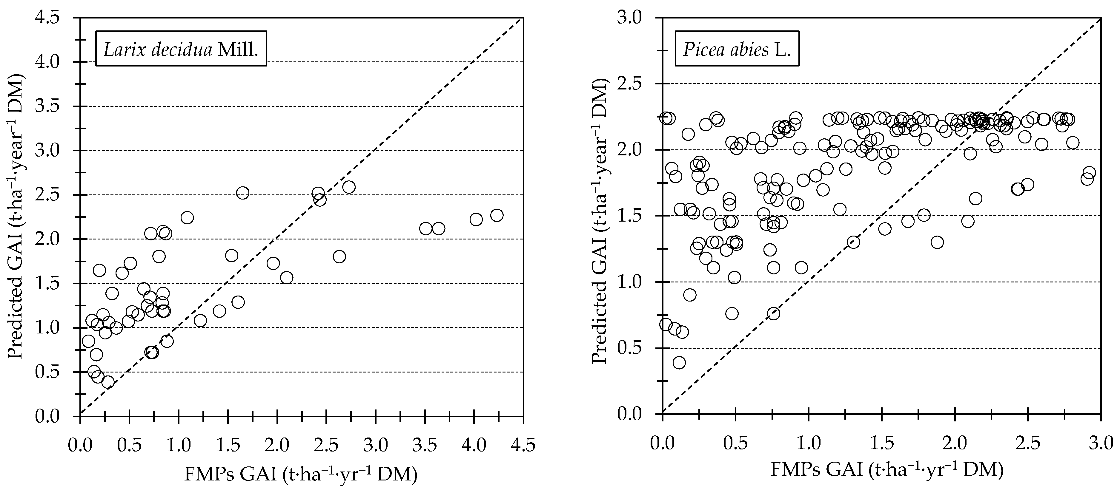
4.1. Gross Annual Increment

A complete validation of the results was not possible due to the following reasons:

• No experimental data were specifically collected for this study by the authors through direct surveys.
• No updated FMPs were made available at the time of the study.

A preliminary validation was then performed by comparing the gross annual increments predicted through the Richards function with those provided by the FMPs (GAI_n(j) and ${\mathrm{GAI}}_{\mathrm{YRs}\left(\mathrm{j}\right)}^{*}$, respectively; t·ha⁻¹·year⁻¹ DM). As an example, Figure 6 shows the comparison between the values of GAI_n(j) and ${\mathrm{GAI}}_{\mathrm{YRs}\left(\mathrm{j}\right)}^{*}$ for Larix decidua Mill. and Picea abies L., which are the most widespread species in the Case Study Area.

While in the case of Larix decidua Mill., underestimation (GAI_n(j) < ${\mathrm{GAI}}_{\mathrm{YRs}\left(\mathrm{j}\right)}^{*}$) and overestimation (GAI_n(j) > ${\mathrm{GAI}}_{\mathrm{YRs}\left(\mathrm{j}\right)}^{*}$) are generally balanced with an r² value equal to 0.71, for Picea abies L. the model causes a systematic overestimation (i.e., the great majority of the values are in the upper half of cartesian field). This undoubtedly represents a very critical aspect that requires further research. In addition to what is already reported in Section 5 (Discussion) regarding the predicted GAI, it is possible that there were unreliable values of FMP GAI present. In the Plans, the increment is generally indirectly estimated by applying statistical methods starting from retrospective measures (generally related to the last 5 or 10 years) of the radial growth of sample trees [56]. Different errors can occur related to both the uncertainty of the measures of the growth and the possible approximation on which the statistical methods are based [57]. However, as this aspect cannot be further investigated here according to the available FMP data, it was not possible to better analyze this eventual source of errors.

Another important aspect that affects the reliability of the values of FMP GAI is that, while for Larix decidua Mill. GAI values were computed through direct measures (except for some stands with protection function with high slope and of difficult access areas), for Picea abies L. several values of FMP GAI were estimated starting from values related to other stands with similar characteristics and under the same ecological–environmental conditions. Moreover, for several stands in the sample, the values of GAI were not made available by the FMP. For all these stands, a value resulting from a weighted average from stands with similar characteristics or derived from the literature was then assigned.

All these elements can affect the values of r² between predicted and provided GAI. To improve the accuracy of the results, it would be desirable if GAI values were always calculated through direct measurements and reported in FMPs with the adopted calculation method.

At the landscape level, a quick comparison between the cumulative merchantable stem mass calculated by WOCAS v2 for the year 2016 and the one estimated by the Mountain Community for the same year showed that the model caused an underestimation of 2.42%, approximately. This means that even if applying the Richards function at the stand level using values of parameters calibrated for the whole Lombardy Region can cause problems of both underestimation and overestimation, at the landscape level these problems can compensate for each other.

4.2. Harvested Merchantable Stem Mass and Utilization Rate

Wood was harvested 4861 times in the period 1994–2018. The total harvested merchantable stem mass, calculated as the sum of the annual harvested mass in each stand, reached 1.44∙10⁵ t DM (18.1% coppice; 81.9% high forest), and the corresponding total C mass was 7.14∙10⁴ t C. Among coppices, wood cuts mainly involved Ostrya carpinifolia Scop. (7.54 × 10³ t DM; 28.9%), Castanea sativa Mill. (4.89 × 10³ t DM; 18.8%), and Fagus sylvatica L. (3.67 × 10³ t DM; 14.1%), whereas among high forests, wood cuts were mainly performed for coniferous (1.07 × 10⁵ t DM; 91.2%) followed by mixed (8.44 × 10³ t DM; 7.2%) and broadleaved (8.00 × 10² t DM; 0.7%) stands, and the main species were Picea abies L. (9.74 × 10⁴ t DM; 82.8%), Larix decidua Mill. (6.66 × 10³ t DM; 5.7%), and Fagus sylvatica L. (5.85 × 10³ t DM; 5.0%).

The weighted average yield of MM_Hn ranged from 0.12 ± 0.22 t·ha⁻¹·year⁻¹ DM (2000) to 4.73 ± 3.22 t·ha⁻¹·year⁻¹ DM (1994). The highest standard deviation (2.68 ± 10.52 t·ha⁻¹·year⁻¹ DM) was reached in 2015, when cuts with high variation in MM_H (from 0.2 to 3.0 × 10³ t·year⁻¹ DM) were performed in similar areas.

At the landscape level, the utilization rate (UR, −), i.e., the ratio between MM_Hn and NAI_n, ranged from 0.02% (2000) to 19.60% (2015). From 1994 to 2001, the maximum value of UR was equal to 6.0%, whereas from 2001 UR increased, even if with considerable differences among the years. Apart from 2015, the highest values were reached in 2012 (19.24%) and 2008 (19.09%) (Figure 7).

These results, in addition to providing an estimation of the available merchantable stem mass at the landscape level over time, can be used as a starting point to assess whether forest management was performed according to sustainable forest management (SFM) approaches and consequently to define future sustainability levels [58]. At the landscape scale, the harvested merchantable stem mass could have been considerably higher without exceeding the net annual increment. Moreover, Figure 7 clearly shows that UR values were highly variable, depending on the management objectives that can change over time according to the characteristics of the stands.

Even if this study presents an analysis at the landscape level, the UR should be assessed case by case for each stand according to its specific characteristics. Moreover, when evaluating the additional mass that could be collected, the multifunctionality of the forests should be considered, as should the impact that an increase in wood cuts might have on other ecosystem services such as the water cycle, soil erosion control, and biodiversity maintenance.

4.3. Aboveground and Belowground Wood Biomass

The total living wood biomass, calculated as the sum of AWB and BWB related to each stand, ranged from 6.73∙10⁴ t DM in 1984 (0.0% coppice; 100.0% high forest) to 5.35∙10⁶ t DM in 2018 (15.0% coppice; 85.0% high forest). TLB_n yield ranged from 44.72 ± 44.42 t·ha⁻¹·year⁻¹ DM in 1984 (81.21% AWB; 18.79% BWB) to 145.49 ± 70.76 t·ha⁻¹·year⁻¹ DM in 2018 (82.12% AWB; 17.88% BWB) (Figure 8). The high standard deviations were due to the inclusion of stands with a high area and low wood biomass, and vice versa. TLB_n yield generally increased year by year for the following reasons: (i) growth of managed stands; (ii) UR < 1; and (iii) inclusion of new stands in the analysis due to the activation of new FMPs. The decrease in TLB yield in 2002 and 2003 compared to 2001 was due both to the inclusion of new stands of large area and low wood biomass, and an increase in the harvested merchantable stem mass of the other stands; for these years, the rate of area increase was higher than the rate of biomass increase while on the contrary the increase in TLB yield in 1991 compared to the previous years was mainly due to the inclusion of new stands characterized by both high area and high wood biomass. In this case, however, the rate of biomass increase was higher than the rate of area increase.

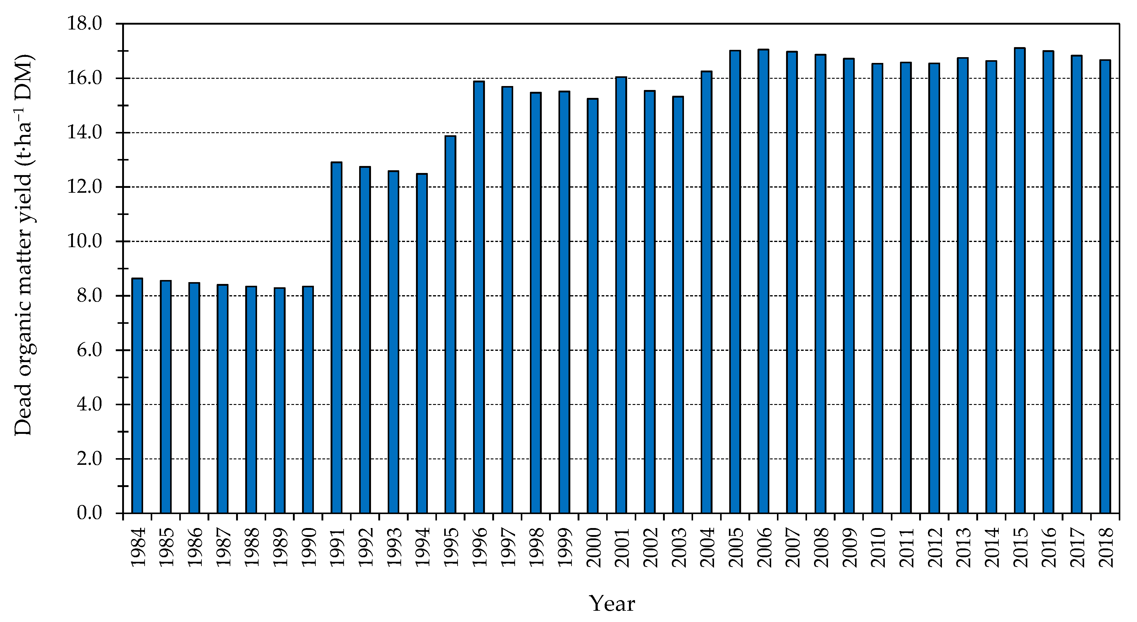
4.4. Dead Organic Matter

The DOM ranged from 1.30∙10⁴ t DM in 1984 (19.31% TLB₁₉₈₄) to 6.12∙10⁵ t DM in 2018 (11.45% TLB₂₀₁₈); DOM yield ranged from 8.28 ± 7.79 t·ha⁻¹·year⁻¹ DM (1989) to 17.11 ± 12.03 t·ha⁻¹·year⁻¹ DM (2015) (Figure 9). The high values of standard deviations can be explained through the same considerations mentioned for living wood biomass. For each year, the mass of the DOM resulted from different processes, i.e., mortality due to self-thinning, production of logging residues, and wood decomposition, the intensity of which varied year by year according to stand characteristics. At the stand level, an increase in wood cuts causes, in the short term, a decrease in the mass of wood in the AWB and a corresponding increase in the DOM mass, and vice versa; at landscape level, however, the DOM mass can undergo further variations if new stands are included in the analysis.

According to [59], the average volume of deadwood in Italian forests amounts to 15.00 m³·ha⁻¹ (7.50 t·ha⁻¹ DM, approximately). On a broader scale, the obtained results can be compared to those reported in [1], showing that the weighted average volume of deadwood at the EU level (year 2015) was 11.50 m³·ha⁻¹, approximately equal to 5.75 t·ha⁻¹ DM, with considerable differences among countries and regions. At the country level, the value ranged from a minimum of 2.30 m³·ha⁻¹ (1.15 t·ha⁻¹ DM) for Portugal to a maximum of 28.00 m³·ha⁻¹ (14.00 t·ha⁻¹ DM) for Slovakia. For regions, the value ranged from a minimum of 5.80 m³·ha⁻¹ (2.90 t·ha⁻¹ DM) to a maximum of 18.40 m³·ha⁻¹ (9.20 t·ha⁻¹ DM), for South-West and Central-West Europe, respectively.

4.5. Carbon Mass

The weighted average C yields in AWB, BWB, and DOM for each year of the analyzed period (t∙ha⁻¹∙year⁻¹ C) are shown in Figure 10. C_AWBn ranged from 18.13 ± 18.30 t∙ha⁻¹∙year⁻¹ C (1984) to 59.10 ± 29.12 t∙ha⁻¹∙year⁻¹ C (2018); C_BWBn ranged from 4.19 ± 4.12 t∙ha⁻¹∙year⁻¹ C (1984) to 12.89 ± 6.64 t∙ha⁻¹∙year⁻¹ C (2018); finally, C_DOMn ranged from 4.13 ± 3.93 t∙ha⁻¹∙year⁻¹ C (1989) to 8.50 ± 6.07 t∙ha⁻¹∙year⁻¹ C (2015). The weighted average C yield (C_TOTn) ranged from 26.63 ± 26.80 t∙ha⁻¹∙year⁻¹ C (1984) to 80.28 ± 41.32 t∙ha⁻¹∙year⁻¹ C (2018), whereas for the whole analyzed period, the weighted average C yield was equal to 67.61 t∙ha⁻¹ C (C_AWB = 72.17%, C_BWB = 15.86% and C_DOM = 11.97%).

The comparison of these results with those obtained from the previous model version for the year 2016 showed that the total C mass increased by 4.94 × 10⁴ t∙year⁻¹ C (+1.78%), i.e., from 2.79 × 10⁶ t∙year⁻¹ C (76.02 t∙ha⁻¹∙year⁻¹ C) to 2.84 × 10⁶ t∙year⁻¹ C (77.37 t∙ha⁻¹∙year⁻¹ C) for the old and new model version, respectively. For the AWB, which is the most relevant C pool, the variation was equal to 2.83 × 10⁵ t∙year⁻¹ C (+15.78%), i.e., from 1.80 × 10⁶ t∙year⁻¹ C (48.86 t∙ha⁻¹∙year⁻¹ C) to 2.08 × 10⁶ t∙year⁻¹ C (56.57 t∙ha⁻¹∙year⁻¹ C) for the old and new model version, respectively. For the neighboring Region of Trentino-Alto-Adige [26], estimated for the period 1995–2011 a weighted average C yield in the aboveground biomass (including leaves) and belowground biomass equal to 90.40 t·ha⁻¹ C and 19.70 t·ha⁻¹ C, respectively. For the same period, according to the analysis performed here, the weighted average C yield in the AWB (excluding leaves) and BWB reached 45.92 t·ha⁻¹ C (−49.20%) and 10.14 t·ha⁻¹ C (−48.53%). These differences may be due to both the application of different approaches as well as to the different structural and compositional characteristics of the forests. For Italy [29], reported for the period 1995–2009 a weighted average C yield for living biomass (aboveground biomass including leaves, and belowground biomass) equal to 65.33 t·ha⁻¹ C, and 18.07 t·ha⁻¹ C for the DOM. For the same period, this work reported a weighted average C yield in living wood biomass equal to 54.93 t·ha⁻¹ C (−15.92%), whereas C yield for the DOM was 8.11 t·ha⁻¹ C (−55.12%). At the EU level [1], the weighted average C yield in the AWB was equal to 51.20 t·ha⁻¹ C (AWB yield: 102.40 t·ha⁻¹ DM), whereas the weighted average C yield in the BWB amounted to 12.80 t·ha⁻¹ C (BWB yield: 25.60 t·ha⁻¹ DM). For South-West Europe, C yield in the AWB was 27.30 t·ha⁻¹ C (AWB yield: 54.60 t·ha⁻¹ DM), whereas C yield in the BWB reached 11.10 t·ha⁻¹ C (BWB yield: 22.20 t·ha⁻¹ DM).

5. Discussion

In this study, specific values of k₁ (wood basic density) for each classification criteria code were used starting from those reported in [31], as these were specific for Italian conditions and available for all the species and management systems considered in this work. Even if these values were published 40 years ago, approximately, they are currently adopted for C accounting at the regional level for the LULUCF sector within the UNFCCC framework [46].

When simulating wood and C stock over time, using constant values of increment may represent quite a strong assumption, especially if the simulation covers a period of a few decades, as in this study. Variations in increment can occur, mainly according to stand volume, environmental conditions, and silvicultural treatments. In order to solve this limitation, in WOCAS v2 the gross annual increment at the stand level is computed through the first derivative of the age-independent theoretical nonlinear Richards function, using the merchantable stem mass as the independent variable. In other words, the increment depends only on the competition within the stands and not on the stand age. This is an advantage compared to the use of age-dependent functions, as it allows estimation of the increment for both even-aged and uneven-aged stands. In addition, several studies have demonstrated that the growth of trees and stands can be computed without considering their age [48,60,61,62,63]. Moreover, as reported by [31,45], age can be used to estimate the increment at the tree level and not for the whole stand where self-thinning, natural disturbances, and felling events result in the presence of trees of different ages within the same stand.

As mentioned before, a complete validation of the results was not possible, and will be performed only when primary stand-level data will be made available through direct surveys or updated FMPs. To this end, a comparison between the values obtained through this analysis and others commonly available in the literature on local, national, and international scales as well as for different periods related to the AWB, BWB, and DOM can represent a first step in validation.

Moreover, in addition to what was previously reported in the results regarding the comparison between predicted and provided GAI, the following aspects must be discussed:

• The gross annual increment is computed in the model using, by default, the values of the parameters calibrated for the whole Lombardy region for each species and management system and as the average value of all the productivity classes, without considering that one class may be prevalent over the others. This means that for stands characterized by different classes the value of the predicted increment is the same; this may represent quite a strong assumption. As reported by [31], the goodness of fit (i.e., the coefficient of determination, or R²) of the Richards function depends on the number of productivity classes; for a given species, as the number of classes increases the R² between increment and volume (or mass) decreases, and vice versa.
• The parameters of the function were estimated in the year 2005 from yield tables produced in the period 1950–1970; it is therefore possible that the increments of the forests might be different today than those related to the period in which the yield tables were produced, due to increases in temperature, CO₂ concentration in the atmosphere, and nitrogen deposition [31].

All of these elements can explain why in some cases (e.g., for Picea abies L.) quite low values of r² can be obtained. Despite this, the values of the parameters of the Richards function used in this study were the only ones currently available for the Lombardy region, and are those used for C accounting at the regional level within the UNFCCC framework. To improve the methodology and the accuracy of the results, it would be desirable to calibrate the growth parameters for each stand in the Case Study Area according to its productivity class; nevertheless, as the information on stand’s productivity is not always made available by the FMPs, estimating the parameters of the Richards function for all the stands is not possible and the only solution at the time of this study was to use average values already applied at the regional level. Including information on stand productivity in the FMPs may help to solve this problem as well as to improve results validation.

Estimating losses due to self-thinning as a fraction of the standing volume, as proposed by [50], can be justified only for a first approximation and if more specific values are not made available. Indeed, both from an ecological perspective and in order to better define the net annual increment as a key variable in SFM, the above-mentioned losses should be estimated as a fraction of the gross increment.

Natural disturbances were not considered in the analysis due to lack of data; the application of WOCAS v2 in other areas where information on disturbances is available would allow detailed analysis of the effect of these processes on forest C dynamics.

In WOCAS v2, the stem mass is converted into total aboveground wood biomass through the parameter k₇ (biomass expansion factor), which represents a key variable in forest C stock assessment. The values of biomass expansion factors vary mainly according to tree size [52,64,65], soil productivity [66], and stand age [67]. This variation is, however, strictly linked to local growth conditions; most of the values available in the literature refer to specific sites and were obtained from a number of trees ranging from ten to a few hundred [66]. As the stem volume is always made available in FMPs, the general approach proposed by [52] was implemented in the model as an alternative method for estimating biomass expansion factors. This approach, however, assumes that young stands are characterized by low volume/mass, and vice versa, even if this situation does not always take place under real conditions; again, stands with the same age can be characterized by different values of stem volume/mass according to their environmental conditions, management, and history. Moreover, the parameters of the regression function were estimated from forests grown under highly variable conditions. Because of this, and because local values should always be preferred, the analysis was performed using the average values of biomass expansion factors reported in [31], as they were specific for Italy and are made available for all of the species and management systems considered in this study.

When evaluating forest management and wood use sustainability, assessing UR is an essential step. According to the principles of SFM, while MM_Hn can exceed NAI_n (UR > 1) in the short term, i.e., when there is a high demand of wood along the supply chain or several phytosanitary cuts of high intensity are performed, in the long term this situation should not be allowed to persist (UR ≤ 1) in order to avoid depletion of stand productivity and biomass over time [1,68,69]. Wood collection is strongly linked to C stock and C sink, and should be considered a positive event if it is performed in compliance with SFM principles. For this purpose, forest management for climate change mitigation can be performed at the stand level to meet the aims of increasing C sink, increasing C stock, and increasing forest resilience and vitality.

The first aim can be achieved by increasing wood collection; in addition to immediately making more biomass available along the supply chain, removing wood reduces the aboveground biomass and promotes the short-term increase of the annual increment, and therefore the C sink. At the same time, increment depends on the merchantable stem mass; therefore, defining a specific value of merchantable mass means defining a specific level of increment and of C sink [45].

On the other hand, the increase of C stock can be achieved through the reduction of wood cuts together with extension of the rotation length [70] in order to maintain a high level of biomass with a low annual increment. The conversion of aged and/or abandoned coppices to high forests is important in meeting this aim, and is useful to obtain high-quality wood for long life-cycle products.

Forest C sink and C stock strongly depend on forest vitality and its resilience to climate change-related impacts, including natural disturbances [8]. To this end, the application of adaptive forest management aimed at increasing stand genetic variability is crucial [71,72,73]. Increasing this variability means increasing biodiversity and enhancing forest conservation, which can be achieved mainly through:

• Increasing of the mass of DOM, which provides micro-habitat for several species of birds, forest-dwelling bats, and mammals, as well as endangered saproxylic beetles [74,75]. In the analysis presented here, the mass of wood in the DOM and the corresponding C mass was computed by assuming that all the producible logging residues were left inside the stands after stem collection. Even if in some cases residues are extracted for energy generation, this assumption can be fully justified as the DOM has a crucial role in reducing soil erosion and water runoff, as well as in releasing nutrient into the soil. Leaving logging residues at the felling site is important because it increases the naturalistic value of the forest while reducing habitat homogenization and soil disturbance [76]. Specific information on the mass of DOM at the stand level is currently missing in the Italian FMPs; including this information would make it possible to collect more detailed data on stand characteristics, allowing improved wood and C mass assessment.
• Maintenance of forest continuity after wood collection, especially as concerns particular forest structural elements (e.g., large and hollow trees) and species composition to sustain different ecological functions [77].
• Conversion of single-species stands to mixed-species stands in order to increase landscape heterogeneity [8,78].
• Restoration of degraded and marginal lands [79], which are generally characterized by high physiognomic–structural disorders, occasional management, and a simplified forest cenosis. In Valle Camonica, this firstly means protecting the so-called “targeted species”, e.g., Acer pseudoplatanus L., Tilia cordata Mill., Ulmus glabra Huds., Ilex aquifolium L., Alnus glutinosa L., and Carpinus betulus L., which mainly colonize abandoned lands and need to be protected through ad hoc practices that, in certain cases, might include limitations on their use [42].

All the above-mentioned practices/measures can be locally supported through specific public incentives. This is particularly important for Valle Camonica, where 66 different forest typologies contribute to the development of a highly heterogeneous ecosystem and landscape. Other practices at the stand level, such as selection cutting for the reduction of fire risk, together with fire monitoring systems and management through prescribed burning and fire suppression, can be performed to limit natural disturbances, even if they might be not suited for biodiversity conservation [8].

Biodiversity protection is extremely important in the context of the SFM and was widely recognized by the recent EU Biodiversity Strategy for 2030 [80]. Forests with a high biodiversity level are more efficient in providing ecosystem services [81,82]. To this end, forest management should recognize the multifunctionality of forests which makes them able to provide, in addition to C sequestration, other services equally important for human well-being and environmental health, such as water regulation, air purification, non-wood products, recreation and tourism usability, and protection against hydrogeological risk and natural hazards. Because of this, forest management should be based on “open management systems” in which different alternatives (e.g., production, biodiversity, and forest conservation) are applied on a case-by-case basis according to the specific characteristics of the stands and the needs of society.

6. Conclusions

Through the WOCAS v2 model it was demonstrated that, if properly managed, FMP data can be used to estimate the mass of wood and C at the stand level, and their variation over space and time for the AWB as well as BWB and DOM, which are not considered in the FMPs. WOCAS v2 uses the merchantable stem mass as the main driver for the calculations, which is always reported in the FMPs; therefore, the model is particularly suitable for use by local decision-makers and forestry authorities, and it can be applied in any forest area where all the required data are made available. This may constitute the basis for further applications on a broader scale.

One of the main improvements in the second version of the model compared to the previous version is that for each stand, calculations can be performed using both the constant gross annual increment provided by the FMPs and a variable one. In this second case, the annual increment is computed through a theoretical non-linear growth function based on the merchantable stem mass without considering the age, solving a limitation of WOCAS v1 in which the gross annual increment was considered as constant (i.e., with the assumption that the stand is in equilibrium and without any dynamic effect). This can be helpful to decision-makers and local authorities for C stock assessment and for addressing specific policies and measures aimed at improving forest management. Moreover, compared to the previous version of the model, in the new version the C stock in the DOM is computed more correctly by considering the transfer of wood and C to this pool due to self-thinning, natural disturbances, and logging residues, as they cause a reduction in C stock in the AWB, but they cause a corresponding increase in C stock in the DOM, and this is quite important for analysis at the stand level.

References

1. Forest Europe. State of Europe’s Forests 2020. Available online: https://foresteurope.org/wp-content/uploads/2016/08/SoEF_2020.pdf (accessed on 30 July 2021).
2. UNFCCC. The United Nations Framework Convention on Climate Change. 1992. Available online: https://unfccc.int/resource/docs/convkp/conveng.pdf (accessed on 17 May 2021).
3. Grassi, G.; Pilli, R.; House, J.; Federici, S.; Kurz, W.A. Science-based approach for credible accounting of mitigation in managed forests. Carbon Balance Manag. 2018, 13, 8. [Google Scholar] [CrossRef] [Green Version]
4. Kurz, W.A.; Birdsey, R.A.; Mascorro, V.S.; Greenberg, D.; Dai, Z.; Olguín, M.; Colditz, R. Integrated Modeling and Assessment of North American Forest Carbon Dynamics: Tools for Monitoring, Reporting and Projecting Forest Greenhouse Gas Emissions and Removals; Commission for Environmental Cooperation: Montreal, QC, Canada, 2016; p. 125. [Google Scholar] [CrossRef]
5. Masera, O.R.; Garza-Caligaris, J.F.; Kanninen, M.; Karjalainen, T.; Liski, J.; Nabuurs, G.J.; Pussinen, A.; De Jong, B.H.J.; Mohren, G.M.J. Modeling carbon sequestration in afforestation, agroforestry and forest management projects: The CO2FIX V.2 approach. Ecol. Model. 2003, 64, 177–199. [Google Scholar] [CrossRef]
6. Morison, J.; Matthews, R.; Miller, G.; Perks, M.; Randle, T.; Vanguelova, E.; White, M.; Yamulki, S. Understanding the Carbon and Greenhouse Gas Balance of Forests in Britain; Forestry Commission: Edinburgh, UK, 2012; p. 160. Available online: https://www.forestresearch.gov.uk/documents/953/FCRP018.pdf (accessed on 13 February 2021).
7. Seidl, R.; Schelhaas, M.J.; Rammer, W.; Verkerk, P.J. Increasing forest disturbances in Europe and their impact on carbon storage. Nat. Clim. Chang. 2014, 4, 806–810. [Google Scholar] [CrossRef] [Green Version]
8. EASAC. Multi-Functionality and Sustainability in the European Union’s Forests; German National Academy of Sciences Leopoldina Editions: Halle (Saale), Germany, 2017; p. 51. Available online: https://easac.eu/fileadmin/PDF_s/reports_statements/Forests/EASAC_Forests_web_complete.pdf (accessed on 30 July 2021).
9. Twery, M.; Weiskittel, A.R. Forest Management Modelling. In Environmental Modelling: Finding Simplicity in Complexity, 2nd ed.; Wainwright, J., Mulligan, M., Eds.; John Wiley & Sons: Chichester, UK, 2013; pp. 379–398. [Google Scholar] [CrossRef] [Green Version]
10. Vanclay, J.K. Modelling Forest Growth and Yield: Applications to Mixed Tropical Forests, 1st ed.; CAB International: Wallingford, UK, 1994; p. 331. [Google Scholar]
11. Landsberg, J. Modelling forest ecosystems: State of the art, challenges, and future directions. Can. J. For. Res. 2003, 33, 385–397. [Google Scholar] [CrossRef]
12. Mäkelä, A.; Landsberg, J.; Ek, A.R.; Burk, T.E.; Ter-Mikaelian, M.; Ågren, G.I.; Oliver, C.D.; Puttonen, P. Process-based models for forest ecosystem management: Current state of the art and challenges for practical implementation. Tree Physiol. 2000, 20, 289–298. [Google Scholar] [CrossRef]
13. Schuck, A.; Päivinen, R.; Hytönen, T.; Pajari, B. Compilation of Forestry Terms and Definitions; European Forest Institute: Joensuu, Finland, 2002; p. 48. Available online: https://efi.int/sites/default/files/files/publication-bank/2018/ir_06.pdf (accessed on 17 May 2021).
14. Mitchell, K.J. Dynamics and simulated yield of Douglas-fir. For. Sci. Monogr. 1975, 17, 1–39. [Google Scholar]
15. Monserud, R.A.; Sterba, H.; Hasenauer, H. The Singletree Stand Growth Simulator PROGNAUS; General Technical Report INT-GTR-373; USDA Forest Service Intermountain Research Station: Fort Collins, CO, USA, 1997; pp. 50–56. [Google Scholar]
16. Pretzsch, H.; Biber, P.; Ďurský, J. The single tree-based stand simulator SILVA: Construction, application and evaluation. For. Ecol. Manag. 2002, 162, 3–21. [Google Scholar] [CrossRef]
17. Crookston, N.L.; Dixon, G.E. The Forest Vegetation Simulator: A review of its applications, structure, and content. Comput. Electron. Agric. 2005, 49, 60–80. [Google Scholar] [CrossRef]
18. Solomon, D.S.; Herman, D.; Leak, W. FIBER 3.0: An Ecological Growth Model for Northeastern Forest Types; General Technical Report NE-204; USDA Forest Service: Durham, NH, USA, 1995; p. 24. Available online: https://www.fs.fed.us/ne/newtown_square/publications/technical_reports/pdfs/scanned/gtr204.pdf (accessed on 13 February 2021).
19. Alder, D. Growth modelling for mixed tropical forests. In Tropical Forestry Papers Number 30; Oxford Forestry Institute Department of Plant Science: Oxford, UK, 1995; p. 231. Available online: http://www.bio-met.co.uk/pdf/TFP30_scan.pdf (accessed on 13 February 2021).
20. Curtis, R.O.; Clendenen, G.W.; DeMars, D.J. A New Stand Simulator for Coast Douglas-Fir: DFSIM User’s Guide; General Technical Report PNW-128; USDA Forest Service Pacific Northwest Research Station: Portland, OR, USA, 1981; p. 83. Available online: https://www.fs.fed.us/pnw/olympia/silv/publications/opt/221_CurtisEtal1981.pdf (accessed on 13 February 2021).
21. García, O. TADAM: A dynamic whole-stand approximation for the TASS growth model. For. Chron. 2005, 81, 575–581. [Google Scholar] [CrossRef]
22. MacPhee, B.; McGrath, T.P. Nova Scotia Growth and Yield Model Version 2: User’s Manual Report FOR 2006-3 No. 79; Nova Scotia Department of Natural Resources: Halifax, NS, Canada, 2006; p. 15. Available online: https://novascotia.ca/natr/library/forestry/reports/REPORT79.PDF (accessed on 13 February 2021).
23. Böttcher, H.; Kurz, W.A.; Freibauer, A. Accounting of forest carbon sink and sources under a future climate protocol-factoring out past disturbance and management effects on age-class structure. Environ. Sci. Policy 2008, 11, 669–686. [Google Scholar] [CrossRef]
24. Verkerk, P.J.; Anttila, P.; Eggers, J.; Lindner, M.; Asikainen, A. The realisable potential supply of woody biomass from forests in the European Union. For. Ecol. Manag. 2011, 261, 2007–2015. [Google Scholar] [CrossRef]
25. Pretzsch, H.; Grote, R.; Reineking, B.; Rotzer, T.; Seifert, S. Models for forest ecosystem management: A European perspective. Ann. Bot. 2008, 101, 1065–1087. [Google Scholar] [CrossRef]
26. Pilli, R.; Grassi, G.; Cescatti, A. Historical analysis and modeling of forest carbon dynamics through the Carbon Budget Model: An example for the Autonomous Province of Trento. For. J. Silvicult. For. Ecol. 2014, 11, 20–35. [Google Scholar] [CrossRef]
27. Böttcher, H.; Verkerk, P.J.; Mykola, G.; Havlik, P.; Grassi, G. Projection of the future EU forest CO2 sink as affected by recent bioenergy policies using two advanced forest management models. GCB Bioenergy 2012, 4, 773–783. [Google Scholar] [CrossRef] [Green Version]
28. Kim, M.; Lee WKKurz, W.A.; Kwak, D.A.; Morken, S.; Smyth, C.E.; Ryu, D. Estimating carbon dynamics in forest carbon pools under IPCC standards in South Korea using CBM-CFS3. iForest Biogeosci. For. 2016, 10, 83–92. [Google Scholar] [CrossRef] [Green Version]
29. Pilli, R.; Grassi, G.; Kurz, W.A.; Smyth, C.E.; Blujdea, V. Application of the CBM-CFS3 model to estimate Italy’s forest carbon budget, 1995–2020. Ecol. Model. 2013, 266, 144–171. [Google Scholar] [CrossRef]
30. Anfodillo, T.; Pilli, R.; Salvadori, I. Preliminary Analysis on the Carbon Stock of the Veneto Region Forests; Direzione Foreste ed Economia Montana: Mestre, Italy, 2006; p. 125. [Google Scholar]
31. Federici, S.; Vitullo, M.; Tulipano, S.; De Lauretis, R.; Seufert, G. An approach to estimate carbon stocks change in forest carbon pools under the UNFCCC: The Italian case. iForest Biogeosci. For. 2008, 1, 86–95. [Google Scholar] [CrossRef] [Green Version]
32. FAO. Guidelines for the Management of Tropical Forests. 1. The Production of Wood. Guidelines for Forest Management Planning. FAO Forestry Paper No. 135. 1998. Available online: http://www.fao.org/3/W8212E/w8212e07.htm#3%20guidelines%20for%20forest%20management%20planning (accessed on 12 October 2020).
33. Dalla Valle, E.; Lamedica, S.; Pilli, R.; Anfodillo, T. Land Use Change and Forest Carbon Sink Assessment in an Alpine Mountain Area of the Veneto Region (Northeast Italy). Mt. Res. Dev. 2009, 29, 161–168. [Google Scholar] [CrossRef]
34. Pilli, R.; Anfodillo, T. Inventory data usage in carbon stock assessment for targeting Kyoto protocol requests. For. J. Silvicult. For. Ecol. 2006, 3, 22–38. [Google Scholar] [CrossRef] [Green Version]
35. Camia, A.; Giuntoli, J.; Jonsson, K.; Robert, N.; Cazzaniga, N.; Jasinevičius, G.; Avitabile, V.; Grassi, G.; Barredo Cano, J.I.; Mubareka, S. The Use of Woody Biomass for Energy Production in the EU; Publications Office of the European Union: Luxembourg, 2021; p. 182. [Google Scholar] [CrossRef]
36. Ciccarese, L.; Pellegrino, P.; Pettenella, D. A new principle of the European Union forest policy: The cascading use of wood products. Ital. J. For. Mt. Environ. 2014, 69, 285–290. [Google Scholar] [CrossRef] [Green Version]
37. Kühmaier, M.; Stampfer, K. Development of a multicriteria decision support tool for energy wood supply management. Croat. J. For. Eng. 2012, 33, 181–198. [Google Scholar]
38. Nonini, L.; Fiala, M. Harvesting of wood for energy generation: A quantitative stand-level analysis in an Italian mountainous district. Scand. J. For. Res. 2021, 36, 474–490. [Google Scholar] [CrossRef]
39. Thiffault, E.; Béchard, A.; Paré, D.; Allen, D. Recovery rate of harvest residues for bioenergy in boreal and temperate forests: A review. WIREs Energy Environ. 2014, 4, 429–451. [Google Scholar] [CrossRef]
40. Canals Revilla, G.G.; Gutierrez del Olmo, E.V.; Picos Martin, J.; Voces Gonzalez, R. Carbon storage in HWPS. Accounting for Spanish particleboard and fiberboard. For. Syst. 2014, 23, 225–235. [Google Scholar] [CrossRef] [Green Version]
41. Sathre, R.; O’Connor, J. Meta-analysis of greenhouse gas displacement factors of wood product substitution. Environ. Sci. Policy 2010, 13, 104–114. [Google Scholar] [CrossRef]
42. Nonini, L.; Fiala, M. Estimation of carbon storage of forest biomass for voluntary carbon markets: Preliminary results. J. For. Res. 2021, 32, 329–338. [Google Scholar] [CrossRef] [Green Version]
43. IPPC. 2006 IPCC Guidelines for National Greenhouse Gas Inventories. Volume 4: Agriculture, Forestry, and Other Land Use. Chapter 2. Generic Methodologies Applicable to Multiple Land-Use Categories. 2006. Available online: https://www.ipcc-nggip.iges.or.jp/public/2006gl/pdf/4_Volume4/V4_02_Ch2_Generic.pdf (accessed on 13 February 2021).
44. Richards, F.J. A Flexible growth function for empirical use. J. Exp. Bot. 1959, 10, 290–301. [Google Scholar] [CrossRef]
45. Tulipano, S. Implementation of a Model to Estimate the Main Carbon Stocks and Flows of Italian Forests for the Purpose of Assessing Their Impact on Mitigation Policies. Master’s Thesis, University of Tuscia, Viterbo, Italy, 2005; p. 179. [Google Scholar]
46. Vitullo, M.; Federici, S. National Forestry Accounting Plan (NFAP)—Italy; Institute for Environmental Protection and Research Editions: Rome, Italy, 2018; p. 191. Available online: https://www.minambiente.it/sites/default/files/archivio/allegati/clima/NFAP_final.pdf (accessed on 23 June 2019).
47. Pienaar, L.V.; Turnbull, K.J. The Chapman-Richards generalization of von Bertalanffy’s growth model for basal area growth and yield in even-aged stands. For. Sci. 1973, 19, 2–22. [Google Scholar] [CrossRef]
48. Zeide, B. Analysis of Growth Equations. For. Sci. 1993, 39, 594–616. [Google Scholar] [CrossRef]
49. Kuusela, K. Forest Resources in Europe, 1950–1990; Cambridge University Press: Cambridge, UK, 1994; p. 154. [Google Scholar]
50. Harmon, M.E.; Krankina, O.N.; Yatskov, M.; Matthew, E. Predicting Broad-scale Carbon Stock of Woody Detritus from Plot-Level Data. In Assessment Methods for Soil Carbon, 1st ed.; Lal, R., Kimble, J.M., Follett, R.F., Stewart, B.A., Eds.; Lewis Publishers: Boca Raton, FL, USA, 2001; pp. 533–552. ISBN 9780367397685. [Google Scholar]
51. Piedmont Region. Analysis of Characteristics of Forest Fires and Response Dynamics; University of Turin and Piedmont Region Editions: Turin, Italy, 2010; p. 131. Available online: http://www.regione.piemonte.it/foreste/images/files/pubblicazioni/ind_caratt_incendi.pdf (accessed on 27 November 2019).
52. Teobaldelli, M.; Somogyi, Z.; Migliavacca, M.; Usoltsev, V.A. Generalized functions of biomass expansion factors for conifers and broadleaved by stand age, growing stock and site index. For. Ecol. Manag. 2009, 257, 1004–1013. [Google Scholar] [CrossRef]
53. Mountain Community of Valle Camonica. Sustainable Development Plan and Landscape Marketing for Valle Camonica. 2015. Available online: https://www.bimvallecamonica.bs.it/scheda/piano-di-sviluppo-sostenibile-e-di-marketing-territoriale-della-valle-camonica-pssmt (accessed on 13 October 2021).
54. Del Favero, R. Forest Typology of Lombardy Region; Ecological Framework for the Management of Lombardy Forests; Cierre Editions: Milano, Italy, 2002; p. 510. [Google Scholar]
55. Thomas, S.C.; Martin, A.R. Carbon content of tree tissues: A synthesis. Forests 2012, 3, 332–352. [Google Scholar] [CrossRef] [Green Version]
56. Corona, P. Methods of Inventorying Masses and Wood Increments in Forest Management; ARACNE Editions: Roma, Italy, 2007; p. 126. [Google Scholar]
57. Hellrigl, B. On the calculation of the percentage increments of standing trees. Ital. J. For. Mt. Environ. 1969, 24, 187–191. [Google Scholar]
58. Marchetti, M.; Motta, R.; Pettenella, D.; Sallustio, L.; Vacchiano, G. Forests and forest-wood system in Italy: Towards a new strategy to address local and global challenges. For. J. Silvicult. For. Ecol. 2018, 15, 41–50. [Google Scholar] [CrossRef] [Green Version]
59. Puletti, N.; Canullo, R.; Mattioli, W.; Radosław, G.; Piermaria, C.; Janusz, C. A dataset of forest volume deadwood estimates for Europe. Ann. For. Sci. 2019, 76, 68. [Google Scholar] [CrossRef]
60. Birch, C.P.D. A New Generalized Logistic Sigmoid Growth Equation Compared with the Richards Growth Equation. Ann. Bot. 1999, 83, 713–723. [Google Scholar] [CrossRef] [Green Version]
61. Chrimes, D. Stand Development and Regeneration Dynamics of Managed Uneven-Aged Picea abies Forests in Boreal Sweden. Ph.D. Thesis, Swedish University of Agricultural Sciences, Umeå, Sweden, 2004; p. 25. Available online: https://pub.epsilon.slu.se/486/1/silvestria304.pdf (accessed on 13 February 2021).
62. Lähde, E.; Laiho, O.; Norokorpi, Y.; Saksa, T. Structure and yield of all-sized and even-sized conifer-dominated stands on fertile sites. Ann. For. Sci. 1994, 51, 97–109. [Google Scholar] [CrossRef] [Green Version]
63. Thrower, J.S. Change Monitoring Inventory Pilot Project for the Merritt IFPAs. Strategic Implementation Plan Version 2, Prepared for Nicola-Similkameen Innovative Forestry Society Merritt, BC, Canada. 2003. Available online: https://www2.gov.bc.ca/assets/gov/farming-natural-resources-and-industry/forestry/stewardship/forest-analysis-inventory/ground-sample-inventories/vri-audits/mti_417_merritt_ifpa_sampleplanv2_finalreport.pdf (accessed on 13 February 2021).
64. Fang, J.Y.; Chen, A.P.; Zhang, X.Q.; Zhao, S.Q.; Ci, L.J. Calculating forest biomass changes in China. Science 2002, 296, 1359. [Google Scholar] [CrossRef] [Green Version]
65. Satoo, T.; Madgwick, H.A.I. Forest Biomass; Forestry Sciences; Nijhoff, M., Junk, W., Eds.; Springer Science & Business Media: The Hague, The Netherlands, 1982; p. 152. [Google Scholar]
66. Wirth, C.; Schulze, E.D.; Schwalbe, G.; Tomczyk, S.; Weber, G.; Weller, E.; Böttcher, H.; Schumacher, J.; Vetter, J. Dynamik der Kohlenstoffvorräte in den Wäldern Thüringens; Max-Planck Institute for Biogeochemistry: Jena, Germany, 2003; p. 328. [Google Scholar]
67. Lehtonen, A.; Mäkipää, R.; Heikkinen, J.; Sievänen, R.; Liski, J. Biomass expansion factors (BEF) for Scots pine, Norway spruce and birch according to stand age for boreal forests. For. Ecol. Manag. 2004, 188, 211–224. [Google Scholar] [CrossRef]
68. Magnani, F.; Raddi, S. Towards an assessment of tree mortality and net annual increments in Italian forests. Which sustainability for the Italian forestry? For. J. Silvicult. For. Ecol. 2014, 11, 138–148. [Google Scholar] [CrossRef] [Green Version]
69. UNECE; FAO. State of Europe’s Forests 2011: Status and Trends in Sustainable Forest Management in Europe; Forest Europe: Oslo, Norway, 2011; p. 344. Available online: https://www.foresteurope.org/documentos/State_of_Europes_Forests_2011_Report_Revised_November_2011.pdf (accessed on 17 May 2021).
70. Barbati, A.; Ferrari, B.; Alivernini, A.; Quatrini, A.; Merlini, P.; Puletti, N.; Corona, P. Forests and carbon sequestration in Italy. Ital. J. For. Mt. Environ. 2014, 69, 205–212. [Google Scholar] [CrossRef] [Green Version]
71. Koskela, J.; Lefèvre, F. Genetic Diversity of Forest Trees. In Integrative Approaches as an Opportunity for the Conservation of Forest Biodiversity; Kraus, D., Krumm, F., Eds.; European Forest Institute: Freiburg, Germany, 2013; pp. 232–241. Available online: http://www.integrateplus.org/uploads/images/Mediacenter/integrate_book_2013.pdf (accessed on 25 February 2022).
72. Müller-Starck, G. Protection of genetic variability in forest trees. For. Genet. 1995, 2, 121–124. [Google Scholar]
73. Nabuurs, G.J.; Delacote, P.; Ellison, D.; Hanewinkel, M.; Lindner, M.; Nesbit, M.; Ollikainen, M.; Savaresi, A. A New Role for Forests and the Forest Sector in the EU Post-2020 Climate Targets: From Science to Policy 2; European Forest Institute: Joensuu, Finland, 2015; p. 32. Available online: https://efi.int/sites/default/files/files/publication-bank/2019/efi_fstp_2_2015.pdf (accessed on 17 May 2021).
74. Bobiec, A. Living stands and dead wood in the Bialowieza Forest: Suggestions for restoration management. For. Ecol. Manag. 2002, 165, 125–140. [Google Scholar] [CrossRef]
75. Müller, J.; Jarzabek-Müller, A.; Bussler, H.; Gossner, M.M. Hollow beech trees identified as keystone structures for saproxylic beetles by analyses of functional and phylogenetic diversity. Anim. Conserv. 2014, 17, 154–162. [Google Scholar] [CrossRef]
76. European Environment Agency. How Much Bioenergy Can Europe Produce without Harming the Environment? EEA Report 7/2006; European Environment Agency: Copenhagen, Denmark, 2006; p. 72. Available online: https://eea.europa.eu/publications/eea_report_2006_7 (accessed on 20 January 2021).
77. Gustafsson, L.; Baker, S.C.; Bauhus, J.; Beese, W.J.; Brodie, A.; Kouki, J.; Lindenmayer, D.B.; Lõhmus, A.; Martínez Pastur, G.; Messier, C.; et al. Retention Forestry to Maintain Multifunctional Forests: A World Perspective. BioScience 2012, 62, 633–645. [Google Scholar] [CrossRef] [Green Version]
78. Fares, S.; Scarascia Mugnozza, G.; Corona, P.; Palahí, M. Sustainability: Five steps for managing Europe’s forests. Nature 2015, 519, 407–409. [Google Scholar] [CrossRef]
79. Nabuurs, G.J.; Pussinen, A.; van Brusselen, J.; Schelhaas, M.J. Future harvesting pressure on European forests. Eur. J. For. Res. 2007, 126, 391–400. [Google Scholar] [CrossRef]
80. European Commission. EU Biodiversity Strategy for 2030. Bringing Nature Back into Our Lives. 2020. Available online: https://eur-lex.europa.eu/resource.html?uri=cellar:a3c806a6-9ab3-11ea-9d2d-01aa75ed71a1.0001.02/DOC_1&format=PDF (accessed on 29 December 2021).
81. Díaz, S.; Demissew, S.; Joly, C.; Lonsdale, W.M.; Larigauderie, A. A Rosetta Stone for Nature’s Benefits to People. PLoS Biol. 2015, 13, e1002040. [Google Scholar] [CrossRef] [Green Version]
82. TEBB. The Economics of Ecosystems and Biodiversity: Mainstreaming the Economics of Nature: A Synthesis of the Approach, Conclusions and Recommendations of TEEB. Available online: http://www.teebweb.org/wp-content/uploads/Study%20and%20Reports/Reports/Synthesis%20report/TEEB%20Synthesis%20Report%202010.pdf (accessed on 3 March 2022).
Figure 1. Logical framework of WOCAS v2 for parameter selection. Image source: www.pixabay.com (accessed on 1 December 2021).
Sustainability 14 03898 g001
Figure 2. General approach implemented into WOCAS v2 for wood and C stock quantification. Image source: www.pixabay.com (accessed on 1 December 2021).
Sustainability 14 03898 g002
Figure 3. Gross annual increment for (i) Picea abies L., (ii) Abies alba Mill., and (iii) Larix decidua Mill. (left) and for (i) Castanea sativa Mill. (management system: coppice), (ii) Quercus cerris L. (management system: high forest), and (iii) Fagus sylvatica L. (management system: high forest) (right).
Sustainability 14 03898 g003
Figure 4. Gross merchantable stem mass for (i) Picea abies L., (ii) Abies alba Mill., and (iii) Larix decidua Mill. (left) and for (i) Castanea sativa Mill. (management system: coppice), (ii) Quercus cerris L. (management system: high forest), and (iii) Fagus sylvatica L. (management system: high forest) (right).
Sustainability 14 03898 g004
Figure 5. Logical framework for the quantification of the mass of wood corresponding to DOM.
Sustainability 14 03898 g005
Figure 6. Predicted vs. provided increments (year: 2002) for: (i) Larix decidua Mill. (N. stands = 50; weighted average: GAIn(j) = 1.26 ± 0.58 t·ha−1·year−1 DM; GAI YRs j * = 0.89 ± 0.86 t·ha−1·year−1 DM; r2 = 0.71; RMSE = 0.84 t·ha−1·year1 DM) (left) and (ii) Picea abies L. (N. stands = 167; weighted average: GAIn(j) = 1.79 ± 0.45 t·ha−1·year−1 DM; GAI YRs j * = 1.24 ± 0.80 t·ha−1·year−1 DM; r2 = 0.55; MRSE = 0.90 t·ha−1·year−1 DM) (right).
Sustainability 14 03898 g006
Figure 7. Utilization rate of the merchantable stem mass according to year.
Sustainability 14 03898 g007
Figure 8. Living wood biomass yield according to year.
Sustainability 14 03898 g008
Figure 9. DOM yield according to year.
Sustainability 14 03898 g009
Figure 10. Weighted average C yield in AWB, BWB, and DOM according to year.
Sustainability 14 03898 g010