A Novel Combined Model for Short-Term Emission Prediction of Airspace Flights Based on Machine Learning: A Case Study of China

Abstract

In order to improve the capability of situational awareness and operational efficiency by considering environmental impact, a prediction model for short-term flight emissions within en route airspace is proposed in this paper. First, the measurement method of fuel consumption and flight emissions based on actual meteorological data is established, and the pattern of flight emissions is analyzed. Then, an adaptive weighting approach is proposed by considering prediction results obtained from a long–short term memory (LSTM) prediction model and extreme gradient boosting (XGBoost) prediction model, respectively. Taking the Guangzhou area control centre (ACC) AR05 sector in central and southern China as an example, the model is trained and tested on emission datasets with three statistical scales, 60 min, 30 min, and 15 min. The result shows that the combined variable–weight prediction model has the greatest prediction effect compared to six other models. In terms of time scale, the prediction performance is best on the 60 min statistical scale dataset; larger statistical unit magnitudes of emissions during the predicting process show better short-term prediction performance. In addition, the increase in data features when training the model plays an essential role in promoting model accuracy. The model established in this paper has high prediction accuracy and stability, which is capable of providing short-term prediction of airspace flight emissions.

1. Introduction

With the rapid development of the global economy, the demand for air transportation continues to grow, and the air transportation volume has grown rapidly at an average annual growth rate of about 5% in the past 20 years [1]. As the number of flights increases, the impact of pollutant emissions on the environment increases as well. A large number of aviation pollutant emissions damage human health and threaten global climate change. In order to promote the sustainable development of air transport, International Civil Aviation Organization (ICAO), the United States, Europe and China have successively proposed the Aviation System Module Upgrade (ASBU), Next Generation Air Transport System (NexGen), European Single Sky ATM Research (SESAR) and Civil Aviation ATM Modernization Strategy (CAAMS) to deal with their energy-saving and emission reduction plans [2,3], accurately perceive the dynamic evolution law of flight operation emissions in the airspace, assist the formulation of energy-saving and emission-reduction policies based on tactical air traffic flow management, and improve sector structure optimization and dynamic capacity to balance “green” deployment capabilities, which will be an important part of sustainable air traffic management in the future.

At present, the research on aircraft operation emission mainly includes emission measurement, analysis of flight pollutant emission reduction measures, and airspace emission prediction. Emission measurement mainly estimates pollutant emissions in the Landing and Take Off (LTO) and Climb/Cruise Descent (CCD) phases. The representative research analyzes the emission inventory of aircraft operating in large airports in different operation phases [4,5]. Taking a specific aircraft type as an example, researchers analyze and estimate the pollutant emissions of aircraft during the taxiing phase [6,7], the LTO phase [8], the cruise phase [9], and the whole flight process [10]. Air pollutant emissions reduction measures include adjusting the proportion of aircraft type [11], reducing ground operation time [12], adopting continuous descent approach procedures [13], and more. As for the prediction of airspace emissions, China is in its infancy in this research field, with the focus mainly on specific airspaces. Based on the forecasted results of future traffic demand, a medium/long-term prediction model for flight emissions has been established to predict the aviation pollutant emissions of this region over the next five years [14,15]. Considering the greenhouse effect of pollutants and aiming to predict equivalent CO₂ emissions, a prediction model of CO₂ emissions of aircraft in the sector was established; however, the calculation process lacks meteorological information on the airspace, and the accuracy of the original data is insufficient [16].

Emissions from flights in high-altitude airspace can accelerate changes in atmospheric chemistry and micro-particle physics, and have an amplifying effect on climate change [17], which is one of the key issues concerning “green civil aviation”. Moreover, the cruise phase accounts for 80% of the flight time, and most fuel consumption and pollutant emissions occur in this phase. Therefore, it is of great significance to study the pollutant emission characteristics of high-altitude airspace cruise flights. In addition, developed countries in aviation have gradually incorporated energy conservation and emission reduction into the scope of air traffic flow management [18], and the ICAO has adopted a market economy-based strategic plan for energy conservation and emission reduction as the main means of traffic management [19]. Strictly controlling the emissions of flights in the airspace is intended to achieve the goal of energy-saving and emission reduction in the airspace through the flow management method based on the market economy. In addition, the future distribution of flight emissions in airspace is an important decision-making basis for airspace route planning and sector design. Accurate prediction of flight emissions in the airspace is an important prerequisite for scientifically formulating energy-saving and emission reduction policies and an important basis for research into energy savings and emission reduction based on air traffic flow management.

An effective method for accurate short-term prediction of emissions during the cruise phase of high-altitude airspace flights is lacking. Therefore, it is imperative that a short-term prediction method for airspace flight emissions with high prediction accuracy and robust performance be built in order to achieve accurate perception of airspace flight emissions, enhance the situational awareness level with regard to environmental performance, to excavate the mechanisms underlying the operational data, and to improve comprehensive operational airspace efficiency while providing a research basis for optimizing reduction of emissions. The goal is to coordinate the comprehensive performance expectations of aviation operations, such as safety, efficiency, and environmental protection while enriching aviation emission management mechanisms and providing both a scientific basis and technical support for the refined management of airspace and the improvement of the regional atmospheric environment.

In this paper, we propose a new combined model to predict short-term emissions from airspace flights. The organizational structure of this article is as follows. Section 2 describes the flight trajectory data of the study area, the calculation method of flight emissions, and the analysis of airspace flight emissions data. Section 3 discusses the short-term prediction combination model of flight emissions in the airspace. Section 4 describes the prediction results of the model and makes a comparative analysis. Finally, Section 5 presents the main conclusions of this work.

2. Materials and Methods

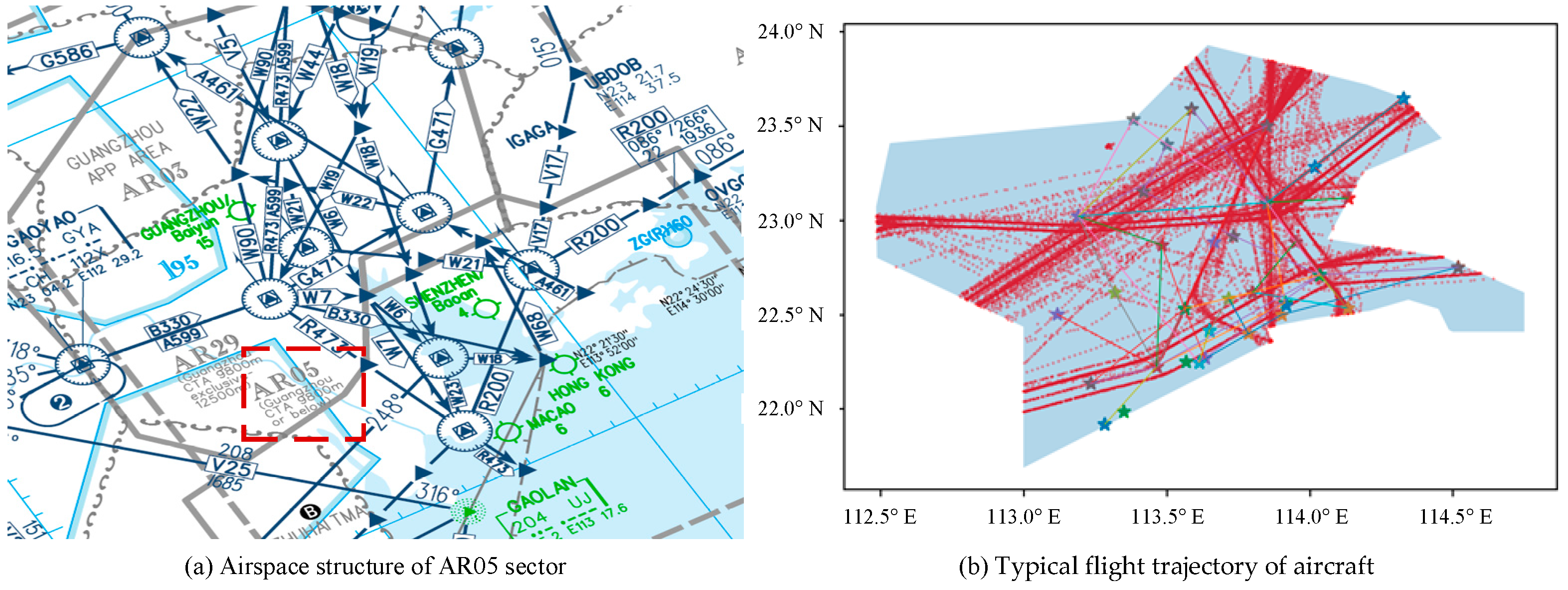
2.1. Study Area and Data Introduction

We took the cruise flight area of flights above 6000 m in AR05 sector under Guangzhou ACC as the research airspace. The airspace belongs to the Civil Aviation Administration of China (CAAC) Central and Southern Regional Administration. This sector has a complex route network and serves nearly 1000 flights every day, including dozens of busy routes such as A461 and R473, carrying flights between Beijing and Guangzhou, and A599, connecting flights between Shanghai and Guangzhou. The Automatic Dependent Surveillance-Broadcast (ADS-B) flight trajectory data from 1 May to 23 May 2019 (UTC time) were selected as the original data for analysis. The trajectory data were from Variflight and covered 86,400 time segments in each working day, processing more than 1.2 million ADS-B in total. The airspace structure of AR05 sector and the typical flight trajectory of aircraft are shown in Figure 1, and the ADS-B trajectory data format is shown in

Table 1. Sample format of ADS-B data.

Callsign	Height	Speed	Longitude	Latitude	…	Time
JT2743	11,308.08	772.97	113.67	23.53	…	14:07:59
JT2743	11,308.08	771.38	113.66	23.55	…	14:08:00
JT2743	11,308.08	770.04	113.65	23.57	…	14:08:01
…	…	…	…	…	…	…
JT2743	11,308.08	767.26	113.64	23.61	…	14:08:23
JT2743	11,308.08	764.61	113.64	23.61	…	14:08:24
JT2743	11,308.08	762.59	113.63	23.64	…	14:08:25

. Based on the grib format meteorological data of the research airspace, the wind speed information and temperature information at the flight position and altitude of the aircraft were extracted. The analyzed wind speed and temperature samples are shown in Figure 2.

2.2. Calculation Method of Flight Emissions in Airspace

Typical aircraft emissions mainly include CO₂, NO_X, CO, HC and SO_X [7]. In this paper, we used the Boeing Fuel Flow Method 2 (BFFM2) method to calculate the emissions of flights, which is more suitable for calculating aircraft emissions during cruise flights. First, the fuel consumption rate of the aircraft operating in the airspace was calculated according to the BADA model [20]; then, the actual emission index was calculated based on the actual operating conditions of the aircraft in order to calculate the emissions of the flight operating in the airspace.

2.2.1. Aircraft Fuel Consumption Calculation Model

This method mainly included the following steps:

(1)

Noise reduction of original trajectory data

Considering that the data quality of ADS-B data is not high, it was necessary to denoise the data before calculating aircraft fuel consumption. Trajectory points with duplicate values in the trajectory data or abnormalities in attributes such as speed, altitude, and monitoring time were deleted.

(2)

Flight key information matching

First, the flight plan data and ADS-B trajectory data were associated through a unique flight identification code to obtain key information such as flight type, airport of departure and landing, actual departure time, etc.

(3)

Judging aircraft flight phase

According to the vertical speed $v_{vertical,i}$ of the ADS-B flight trajectory monitoring point, the trajectory flight phase was divided into three flight phases: climb, cruise, and descent.

Note that the ADS-B flight trajectory monitoring point of the flight is $\left\{P_0,P_1,P_2,P_3,\dots ,P_n\right\}$. $P_i$ is classified into climb, cruise, and descent according to the vertical speed of the trajectory point

$$\{\begin{array}{l}{v}_{vertical,i}<-R{D}_{\min }\\ -R{D}_{\min }\le v_{vertical,i}\le R{C}_{\min }\\ v_{vertical,i}>R{C}_{\min }\end{array}\begin{array}{c},\mathrm{descent}\\ ,\mathrm{cruise}\\ ,\mathrm{climb}\end{array}$$

(1)

where $R{D}_{\min }$ represents the set value of the minimum descent rate and $R{C}_{\min }$ represents the set value of the minimum climb rate. For specific values, refer to [21].

(4)

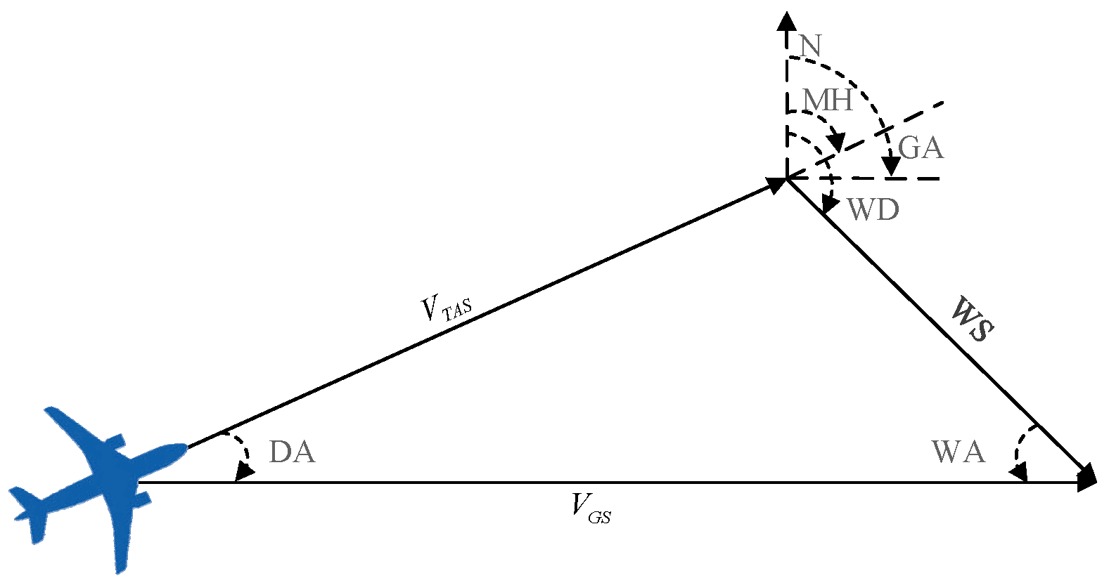
Flight airspeed conversion

Flight airspeed conversion was performed as follows. Convert the flight ground speed, $V_{GS,i}$ in the ADS-B trajectory monitoring data into true airspeed, $V_{TAS,i}$. Extract the wind speed information, ${\mathrm{WS}}_i$ at the location of the flight trajectory point, as shown in Figure 3, and convert the vector of the flight ground speed, $V_{GS,i}$ into true airspeed, $V_{TAS,i}$ according to the Forward Velocity Triangle (FVT).

According to the airspace meteorological data, determine the wind speed, ${\mathrm{WS}}_i$ and wind direction, ${\mathrm{WD}}_i$ at the location of aircraft flight trajectory point, $p_i$ in the corresponding period, considering only the influence of horizontal wind and ignoring the vertical wind. Combined with the ground speed, $V_{GS,i}$, magnetic heading, ${\mathrm{MH}}_i$ and magnetic trajectory angle, ${\mathrm{GA}}_i$ of the trajectory point provided by ADS-B trajectory data, convert the ground speed, $V_{GS,i}$ of the aircraft flight trajectory point into true airspeed, $V_{TAS,i}$. The specific process is as follows:

$$\{\begin{array}{c}{\mathrm{TA}}_i=\left|W{D}_i-{\mathrm{MH}}_i\right|\\ {\mathrm{DA}}_i=\left|{\mathrm{GA}}_i-{\mathrm{MH}}_i\right|\\ {\mathrm{WA}}_i=\mathrm{T}{\mathrm{A}}_i-{\mathrm{DA}}_i\end{array}$$

(2)

$$V_{TAS,i}=\sqrt{V_{GS,i}^2+\mathrm{W}{\mathrm{S}}_i^2-2V_{GS,i}\mathrm{W}{\mathrm{S}}_i\cdot \cos \mathrm{W}{\mathrm{A}}_i}$$

(3)

If ${\mathrm{TA}}_i\ge 180$, then ${\mathrm{TA}}_i=\left|{\mathrm{WD}}_i-{\mathrm{MH}}_i\right|-180$.

(5)

Calculation of actual flight fuel flow rate

We used the BADA model to calculate the flight performance parameters of the aircraft according to the flight phases of the flight trajectory points of the flight. With these main parameters, including lift coefficient, $C_{L,i}$, drag coefficient, $C_{D,i}$, drag, $D_i$ and thrust, $T_i$, the fuel flow rate, $F_{actual,i}$ of the flight under actual operating conditions can be calculated:

$$\{\begin{array}{l} C_{L,i}=\frac{2m_{i}g}{{\rho }_i{V}_{TAS,i}^{2}S}\\ C_{D,i}=C_{D0,cr}+C_{D2,cr}\times {(C_{L,i})}^2\\ D_i=\frac{1}{2}{C}_{D,i}\cdot {\rho }_i\cdot V_{TAS,i}^2\cdot S\end{array}$$

(4)

$${\rho }_i={\rho }_0{(\frac{T_0+\Delta T-\beta h_i}{T_0})}^{-\frac{g}{\beta R}-1}$$

(5)

$$T_i=\{\begin{array}{c}{D}_i+m_{i}g\sin \theta \\ D_i-m_{i}g\sin \theta \\ D_i\end{array}\begin{array}{c},\mathrm{climb}\\ ,\mathrm{descent}\\ ,\mathrm{cruise}\end{array}$$

(6)

$${\eta }_i=C_{f1}\times (1+\frac{V_{TAS,i}}{C_{f2}})$$

(7)

$$F_{actual,i}=\{\begin{array}{l}{f}_{nom,i}={\eta }_i\times T_i\\ f_{min,i}=C_{f3}\times (1-H_{P,i}/C_{f4})\\ f_{CR,i}={\eta }_i\times T_i\times C_{fcr}\end{array}$$

(8)

where $C_{D0,cr}$ and $C_{D2,cr}$ are the aircraft resistance parameters, $m_i$ is the aircraft weight of trajectory point $P_i$ (obtained according to the initial weight difference), $g$ is the gravitational acceleration, ${\rho }_i$ is the atmospheric density of the flight altitude of trajectory point $P_i$, ${\rho }_0$ is the standard atmospheric density at Mean Sea Level (MSL), $T_0$ is the standard atmospheric temperature at MSL, $\Delta T$ is the temperature differential at MSL, $\beta$ is the International Standard Atmosphere (ISA) temperature gradient with altitude below the tropopause, equal to −0.0065 k/m, $h_i$ is the flight altitude, $R$ is the real gas constant for air, equal to 287.053 ${\mathrm{m}}^2/(\mathrm{K}\cdot {\mathrm{s}}^2)$, $S$ is the wing surface area, ${\eta }_i$ is the thrust specific fuel consumption, $H_{P,i}$ is the geopotential pressure altitude at trajectory point P_i, f_nom,i is the climb fuel flow rate, f_min,i is the descent fuel flow rate f_CR,i is the cruise fuel flow rate, and C_f1, C_f2, C_f3, C_f4 and C_fcr are the fuel flow coefficients corresponding to the aircraft.

2.2.2. Aircraft Emissions Calculation Model

The model mainly included the following steps:

• Convert actual fuel flow rate to reference fuel flow rate

Convert the fuel flow rate $F_{actual,i}$ of the aircraft under actual operating conditions to the fuel flow rate $F_{ref,i}$ under reference conditions (temperature 288.15 k, atmospheric pressure 14.696 psi), that is:

$$\{\begin{array}{l}{F}_{ref,i}=(F_{actual,i}/{\delta }_{amb,i}){\theta }_{amb,i}^{3.8}{e}^{0.2M_{{}^i}^2}\\ {\delta }_{amb,i}=P_{amb,i}/14.696\\ {\theta }_{amb,i}=(T_{amb,i}+273.15)/288.15\end{array}$$

(9)

where F_ref,i represents the fuel flow rate of the aircraft under reference meteorological conditions, $P_{amb,i}$ represents the atmospheric pressure under the actual flight conditions of the aircraft, $T_{amb,i}$ represents the ambient temperature at the flight conditions in Kelvin, δ_amb,i represents the ratio of the atmospheric pressure under the actual flight conditions of the aircraft to the reference flight conditions, ${\theta }_{amb,i}$, represents the ratio of the temperature under the actual flight conditions of the aircraft to the reference flight conditions, and $M$ indicates the flight Mach number of the aircraft.

2.

Calculation formula of aircraft emissions

Convert the reference fuel flow rate of the corresponding aircraft model in the Engine Emissions Databank (EEDB) into the corrected fuel flow rate in the LTO phase. Considering that the reference fuel flow rate in the LTO phase provided by EEDB database is measured by the engine under reference conditions, the actual fuel consumption of the aircraft needs to eliminate the influence of installation effects [14] and the corrected fuel flow rate $F_{correct}$ of the aircraft in four states: takeoff (100% thrust condition), climb (85% thrust condition), approach (30% thrust condition), and taxiing (7% thrust condition); thus:

$$F_{correct}=\{\begin{array}{c}{F}_{to}\times 1.010\\ F_{cl}\times 1.013\\ F_{dc}\times 1.020\\ F_{tx}\times 1.100\end{array}$$

(10)

where, $F_{to}$, $F_{cl}$, $F_{dc}$, and $F_{tx}$ respectively represent the reference fuel flow rates under the four states of takeoff, climb, approach, and taxiing in the LTO phase provided by the EEDB database.

In this paper, we mainly calculated the five emissions of aircraft mentioned above. Among them, the emission indexes of CO₂ and SO_X were 3155 g/kg and 0.8 g/kg respectively; these emissions do not change with atmospheric conditions and engine types, while the emission indexes of NOx, CO and HC change with engine types and actual flight conditions.

Taking the B737 aircraft as an example, this paper introduces the calculation process of the emission index under the actual flight conditions of this model. In order to facilitate the calculation, the following assumptions were made:

• The cruise starting weight of each type of aircraft is the reference weight of the Operation Performance File (OPF) in the BADA database;
• The air relative humidity in the study airspace is 65.18% [22];
• The installation and deterioration effects of the aircraft engine are negligible.

According to the ICAO emission database, we obtained the fuel flow rate and emission index of the B737 aircraft engine (CFM56-7B26) in the LTO cycle phase under reference atmospheric conditions, as shown in

Table 2. ICAO emission data for the aviation engine CFM56-7B26.

Mode of the LTO Cycle	Fuel Flow Rate (kg/s)	Reference Emissions Indices (g/kg)
		REIHC	REICO	REINOx
Take off	1.221	0.1	0.2	28.8
Climb	0.999	0.1	0.6	22.5
Approach	0.338	0.1	1.6	10.8
Taxi	0.113	1.9	18.8	4.7

.

Then, based on the basic emission data, the double logarithm relationship between emission index and fuel flow rate was established by BFFM2, as shown in Figure 4.

3.

According to the logarithmic relationship between the reference emission index and the fuel flow rate $F_{ref,i}$ of the aircraft under reference meteorological conditions, the reference emission indexes of NOx, CO, and HC were calculated by linear interpolation, that is, the reference emission index under actual operating conditions.

4.

The emission index under reference conditions was revised to the actual atmospheric conditions. Considering the influence of atmospheric effect, the calculated reference emission index was corrected to the actual atmospheric conditions, namely:

$$\{\begin{array}{l}EIN{O}_x{}_{,i}=REIN{O}_x{e}^{H_i}{({\delta }_{amb,i}^{1.02}/{\theta }_{amb,i}^{3.3})}^{1/2}\\ EIC{O}_i=REICO({\theta }_{amb,i}^{3.3}/{\delta }_{amb,i}^{1.02})\\ EIH{C}_i=REIHC({\theta }_{amb,i}^{3.3}/{\delta }_{amb,i}^{1.02})\\ H_i=-19\times (w_i-0.0063)\end{array}$$

(11)

where $EIN{O}_{x,i}$, $EIC{O}_i$, and $EIH{C}_i$, respectively, represent the emission indexes of NO_x, CO, and HC under actual operating conditions, REINO_x, $REICO$, and $REIHC$, respectively, represent the emission indexes of NO_x, CO, and HC under reference conditions, H_i represents the humidity correction factor under actual operating conditions, and $w_i$ represents the specific humidity under actual operating conditions.

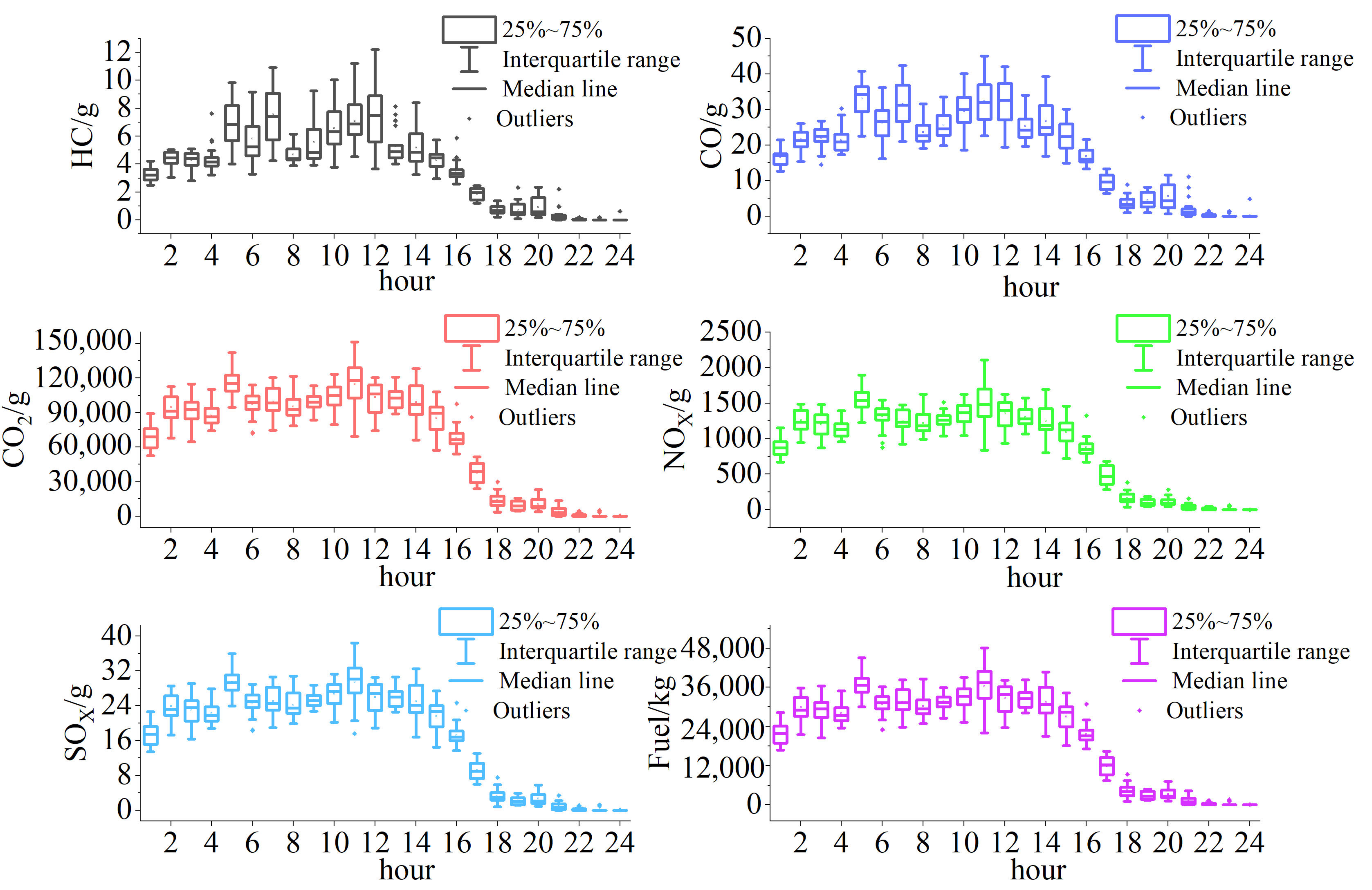
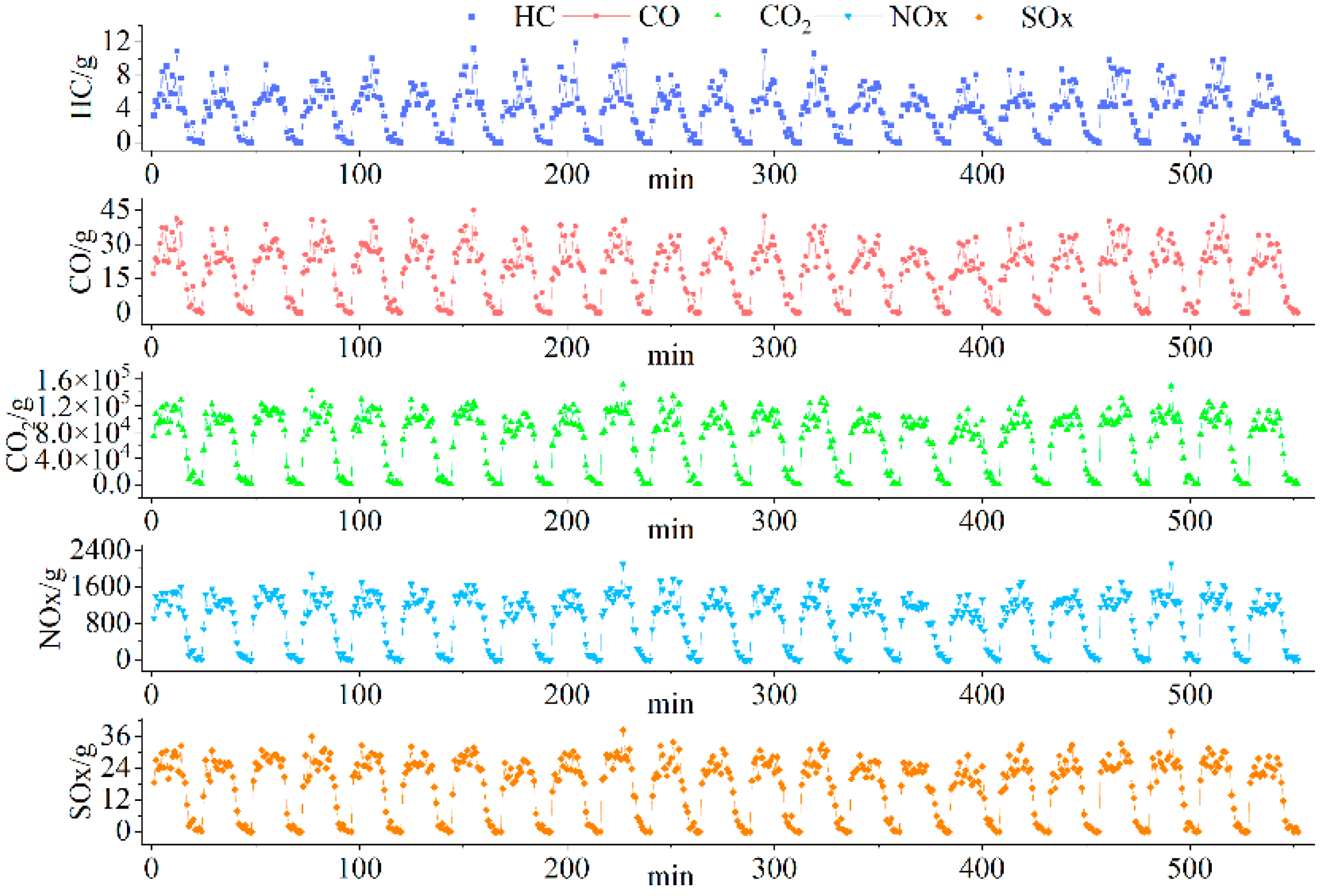
2.3. Analysis of Flight Emission Data in Airspace

We calculated the aircraft fuel flow rate corresponding to each aircraft type in the airspace according to the aircraft fuel consumption calculation model and compared it with the fuel flow rate under the actual operating conditions published in the Flight Crew Operation Manual (FCOM) in order to verify the accuracy of the fuel flow rate of the aircraft type corresponding to the flight. Then, the pollutant emission characteristics of flights operating in the research airspace were analyzed according to the aircraft emission calculation model.

Using the method proposed in this paper, five emissions and fuel consumption in 24 h a day (23 days in total) were calculated and the corresponding distribution of each hour was counted. As shown in Figure 5, the fluctuation trend of the emissions of flights in the sector according to the distribution of the five emissions is similar to that of fuel consumption. The peak emission hours are 6–8 a.m. and 10–12 a.m. every day. After 2 p.m., emissions show a downward trend and the emission trend is essentially consistent with changes in air traffic flow in the sector. This proves that exploring the emission law of pollutants can assist in the formulation of air traffic flow management methods and promote energy conservation and emissions reduction.

As shown in Figure 6, the minute time-series diagram of the five emissions shows that each emission has good periodic characteristics, which provides basic information for short-term pollutant emissions prediction.

In order to further analyze the timing periodicity of the five emissions, the serial correlation function was used for the periodicity test. As shown in Figure 7, the Autocorrelation Values (ACV) corresponding to each of the five emissions have multiple peaks and obvious periodicity.

3. Short Term Prediction Model of Airspace Flight Emissions

Common prediction methods mainly include the time-series analysis method and machine learning algorithms; it has been found that the combined prediction model has better prediction accuracy than the single prediction model [23]. Relevant scholars have used grey prediction, Back Propagation (BP) neural network, Autoregressive Integrated Moving Average (ARIMA), and time-series prediction algorithms such as Support Vector Regression (SVR) as well as machine learning algorithms in combination for prediction [24,25,26]. However, the existing combined forecasting models mostly involve the simple addition of several models and lack interaction between models. In this paper, two single machine learning models are organically combined to make short-term predictions of airspace flight emissions. Considering the weighting problem of the combined forecasting model, an adaptive time-varying weighting method was designed to determine the time-varying weight of a single machine learning forecasting model in order to achieve short-term accurate forecasting of airspace flight emissions.

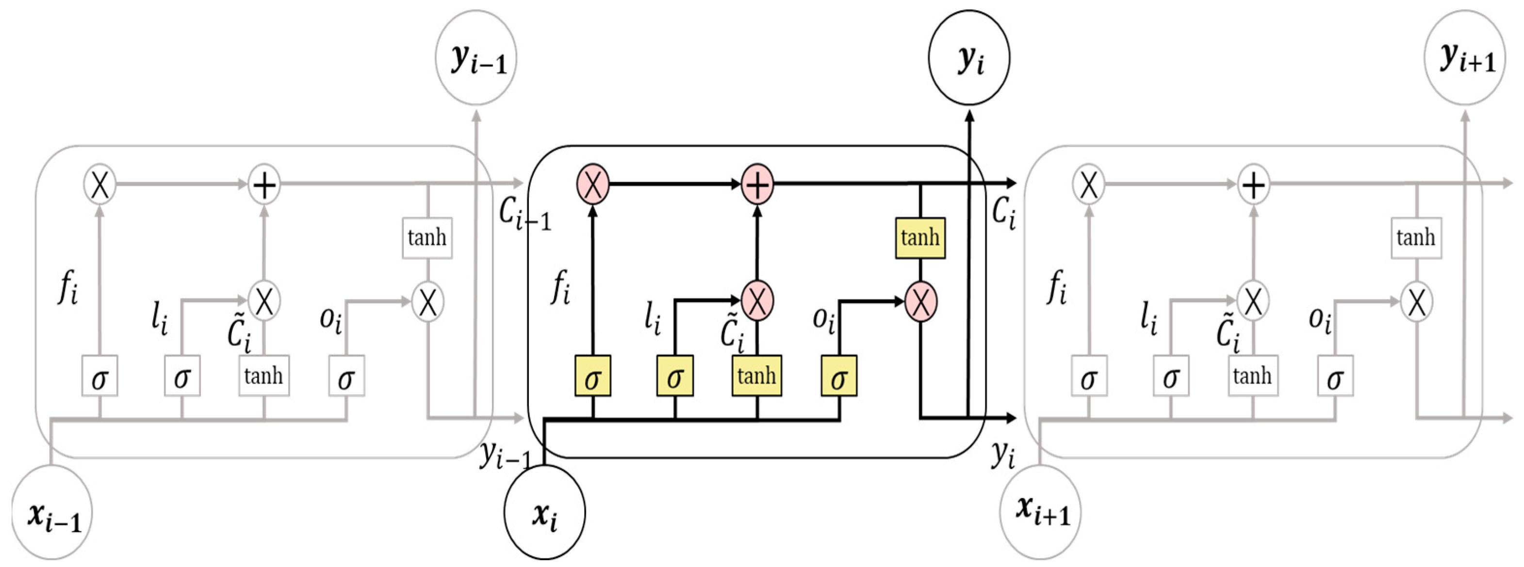
3.1. LSTM Prediction Model

The LSTM is a special kind of cyclic neural network. By introducing a forget gate, input gate, and output gate the model can make up for problems such as insufficient long-term memory and gradient disappearance in Recurrent Neural Networks (RNN), making the network converge better and faster, effectively improving the short-term prediction accuracy of emissions. LSTM applications in traffic [27], electric power [28], environment [29], and other fields are common. The basic network structure is shown in Figure 8, where $C_i$ represents the cell state, $\tanh$ is the hyperbolic tangent activation function, and $\sigma$ is the sigmoid activation function.

The LSTM prediction model was established based on emission training set samples, as follows. First, the forget gate $f_i$ determines the cell state $C_i$ by viewing the emission output value $y_{i-1}$ at time $i-1$ and the emission input value $x_i$ at time $i$, that is:

Forget gate:

$$f_i=\sigma (W_f\cdot \left[y_{i-1},x_i\right]+b_f)$$

(12)

Second, the value and cell status updated inside the cell are determined by the input gate $l_i$, that is:

Input gate:

$$l_i=\sigma (W_l\cdot \left[y_{i-1},x_i\right]+b_l)$$

(13)

Cell state:

$${\tilde{C}}_i=\tanh (W_c\cdot \left[y_{i-1},x_i\right]+b_C)$$

(14)

$$C_i=f_i\otimes C_{i-1}+i_i\otimes {\tilde{C}}_i$$

(15)

Finally, the output gate determines the output of the emission at the current time $i$, that is:

Output gate:

$$o_i=\sigma (W_o\cdot \left[y_{i-1},x_i\right]+b_o)$$

(16)

Final output:

$$y_i=o_i\otimes \tanh (C_i)$$

(17)

where f_i $l_i$, ${\tilde{C}}_i$, $C_i$, $o_i$, $x_i$ and $y_i$, respectively, represent the forget gate, input gate, previous cell state, current cell state, output gate, input, and output at time $i$; $W_f$, $W_l$, $W_c$, and $W_o$ represent the matrix weights of the forget gate, input gate, cell state, and output gate, respectively; $b_f$, $b_l$, $b_C$, and $b_o$ represent the offset items of the forget gate, input gate, cell state, and output gate, respectively.

3.2. XGBoost Prediction Model

XGBoost is an integrated learning algorithm based on decision trees. Based on the gradient lifting tree model, it integrates many cart regression tree models to form a strong classifier, which can improve the ability of the prediction model and has achieved good results in the field of short-term traffic flow prediction [30]. XGBoost adds a regular term to the cost function based on the traditional boosting model and makes a second-order Taylor expansion of the cost function. It automatically learns the splitting direction and supports column sampling to control the complexity of the model. The trained model is simpler and can prevent overfitting. The XGBoost model tool supports parallel processing and can calculate multi-threaded gain of each feature to reduce learning time. With these advantages, the XGBoost algorithm shows strong ability in various regression prediction problems. Its prediction model can be expressed as

$${\widehat{y}}_i={\displaystyle \sum {}_{k=1}^K}{f}_k(x_i),f_k\in F$$

(18)

where ${\widehat{y}}_i$ refers to the ith prediction value of sample emission $x_i$, K refers to the number of decision trees, $f_k$ refers to the kth decision tree, and F refers to the set space of CART regression tree.

In each iteration the original model remains unchanged, a new tree model is added to the original model, and the newly-generated tree model is used to fit the last prediction residual value. The specific iterative process can be expressed as follows:

$$\{\begin{array}{l}{\widehat{y}}_i^{(0)}=0\\ {\widehat{y}}_i^{(1)}={\widehat{y}}_i^{(0)}+f_1(x_i)\\ \hspace{1em}\hspace{1em}\hspace{1em}\hspace{1em}⋮\\ {\widehat{y}}_i^{(k)}={\widehat{y}}_i^{(k-1)}+f_k(x_i)\end{array}$$

(19)

The objective function is expressed as follows:

$$J_{obj}={\displaystyle \sum {}_{i=1}^n}l(y,\widehat{y})+{\displaystyle \sum {}_{i=1}^K}\mathsf{\Omega }(f_k)$$

(20)

where ${\displaystyle \sum {}_{i=1}^n}l(y,\widehat{y})$ is the difference between the predicted value and the true value of the model and ${\displaystyle \sum {}_{i=1}^K}\mathsf{\Omega }(f_k)$ represents the regular term of the objective function.

For the regular term of the objective loss function, the regular term of the k decision tree is:

$$\mathsf{\Omega }(f_k)=\gamma T+\frac{1}{2}\lambda {\displaystyle \sum {}_{j=1}^T}{w}_j^2$$

(21)

where $\gamma$ represents the penalty function coefficient, T represents the number of leaf nodes, $\lambda$ is used to regulate the score value of leaf nodes, and $w_j$ is the score value of the jth sub node.

3.3. Combined Forecasting Model

3.3.1. Weighting Method of Combined Forecasting Model

Combined prediction is the combination of several different prediction models, which can often integrate the advantages of different models and greatly improve prediction accuracy. The combined prediction model focuses on determining the weighting coefficient of each model. Commonly-used methods include the arithmetic average weighting method (AAWM), reciprocal variance weighting method (RVWM), and optimal weighting method (OWM). In this paper, we used the RVWM to determine the prediction weight of the LSTM prediction model and XGBoost prediction model at each time and then makes adaptive improvements, specifically as follows:

(1)

RVWM

$$\{\begin{array}{l}f(x_t)=\frac{1}{n}{\displaystyle \sum {}_{i=1}^n}{w}_i(t-1)f_i(x_t)\\ w_i(t)=\frac{1/e_{it}}{{\displaystyle \sum {}_{i=1}^n(1/e_{it})}}\\ e_{it}=y_t-f_i(x_t)\\ s.t.{\displaystyle \sum {}_{i=1}^n{w}_i(t-1)=1,w_i(t-1)\ge 0}\end{array}$$

(22)

where $w_i(t-1)$ is the weight of the ith model at t − 1 time, $y_t$ represents the true value of the feature at t time, and $e_{it}$ is the prediction error of the ith model at t time.

(2)

Adaptive time-varying weighting model (ATVWM)

First, the prediction weight of the LSTM prediction model and XGBoost prediction model at each time was used, then the combined optimization model was used to determine the optimal number m and weight coefficient with the minimum prediction error, that is:

$$\{\begin{array}{l}\min J_t=\left|e_t\right|=\left|{\displaystyle \sum {}_{i=1}^n{W}_{it}{e}_{it}^{\ast }}\right|\\ s.t.{\displaystyle \sum {}_{i=1}^n{W}_{it}=1,W_{it}\ge 0}\end{array}$$

(23)

$$W_{i,m+1}=\frac{1}{m}{\displaystyle \sum {}_{t=1}^m}{W}_{it},W_{i,m+2}=\frac{1}{m}{\displaystyle \sum {}_{t=1}^{m+1}}{W}_{it},\dots ,W_{i,m+j}=\frac{1}{m}{\displaystyle \sum {}_{t=1}^{m+j-1}}{W}_{it}$$

(24)

where $W_{it}$ represents the weight coefficient of the ith model at time t. Then, for time t, calculate the absolute error values $w_i(t)$ and $W_{it}$ between the predicted value and the true value of the combined prediction model, corresponding to $e_{it}$ and $e_{it}^{\ast }$, compare the size of the two, and adjust the adaptive weight; that is, if $e_{it}$ < $e_{it}^{\ast }$, use weight $W_{it}$ to replace the original weight, $w_i(t)$.

3.3.2. Weighting Method of Combined Forecasting Model

As shown in Figure 9, the research framework for combined prediction of airspace flight emissions was mainly composed of five parts: database, data processing, prediction model, prediction results, and performance analysis. The experiment was run on a 64-bit Microsoft Windows 10 operating system. The processor was an Intel (R) core (TM) i7-10510u CPU @ 1.80 GHz, 2.30 GHz, 16 GB memory and 512 GB SSD. All experiments were performed with Python Anaconda 3.9, and the software architecture was developed based on a deep learning library tool based on Keras. The details are as follows:

(1)

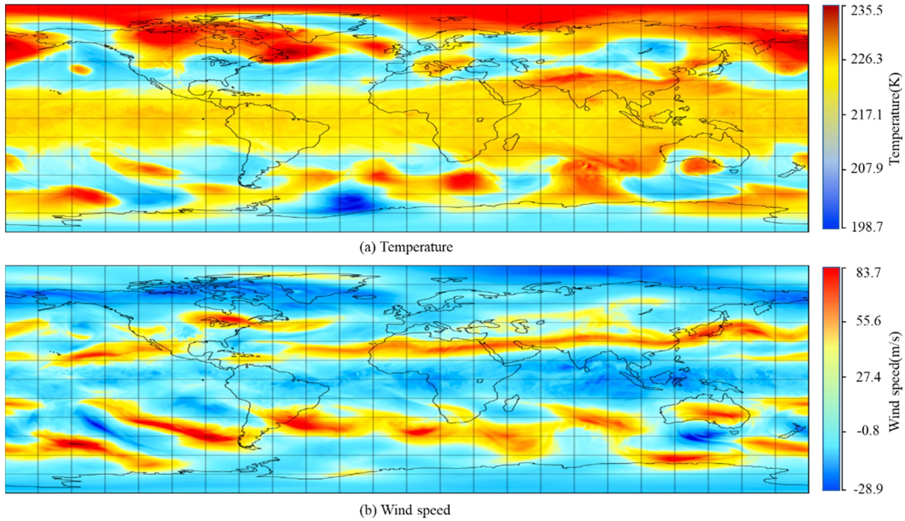
Database: based on the BADA model performance database (weight of aircraft and performance parameters), EEDB emission database, airspace information, meteorological information (atmosphere temperature, wind speed, and direction), flight plan information, and aircraft ADS-B flight trajectory data.

(2)

Data processing: an aircraft fuel consumption calculation model and aircraft emission calculation model were used to calculate the time-series data set of flight emissions in the airspace.

(3)

Prediction model: the data set was divided according to the proportion training set:test set = 9:1, then the LSTM prediction model and XGBoost prediction model were trained and five comparative single machine learning prediction models set up, including a Random Forest model (RF), Artificial Neural Network model (ANN) and Support Vector Machine model (SVM), to confirm the rationality of selecting the LSTM and XGBoost prediction models. The training prediction model determined the super parameters. The super parameters of the LSTM and XGBoost prediction models were determined as follows:

Additional layers in the neural network module of the LSTM prediction model provide stronger learning ability. However, too many layers can easily make it difficult to converge during network training. During the training process, the number of network layers is generally set to two layers [31]. With the two-layer network is set, the activation function was sigmoid, network training used the Adam optimization algorithm, the learning rate was set at 0.001–0.01, the number of iterative training sessions was 200, and the batch size was set at 10–100.

The XGBoost prediction model requires two kinds of general parameters, namely, weak evaluator parameters and task parameters, during training. Among them, weak evaluator parameters have the greatest impact on algorithm performance, mainly affecting learning rate, maximum depth of tree, training sample sampling rate, etc. Task parameters mainly affect the learning target, random number seed, etc. [32]. The learning rate was set at 0.01–0.1, the maximum depth of the tree was 2–5, the maximum number of iterations of the weak learner was 100–10,000, the training sample sampling rate was 0–0.9, the random number seed was 100–1000, and other parameters were set according to initialization.

We used the grid search method [33] provided by scikit-learn to determine the optimal super parameters of the above model and save the training model. Then, a combined prediction model weighting method was designed which integrates the prediction results of two single machine learning models, namely, the LSTM network and the XGBoost model.

(4)

Prediction results: the short-term prediction results of airspace flight emissions over 1 h, 30 min, and 15 min were calculated according to the established variable weight combination prediction model.

(5)

Performance analysis: the prediction performance of each prediction model was evaluated according to the performance evaluation index.

3.4. Model Prediction Performance Index

In the prediction problem, the generally selected performance evaluation indexes were as follows:

(1)

Root mean square error (RMSE)

$$RMSE=\sqrt{\frac{1}{n}{\displaystyle \sum {}_{i=1}^n{(y_i-{\widehat{y}}_i)}^2}}$$

(25)

(2)

Mean Absolute Error (MAE)

$$MAE=\frac{1}{n}{\displaystyle \sum {}_{i=1}^n}\left|y_i-{\widehat{y}}_i\right|$$

(26)

(3)

Coefficient of Determination (R²)

$$R^2=1-\frac{{\displaystyle {\sum }_{i=1}^n{({\widehat{y}}_i-y_i)}^2}}{{\displaystyle {\sum }_{i=1}^n{(y_i-\overline{y})}^2}}$$

(27)

where n represents the quantity of sample data, ${\widehat{y}}_i$ represents the predicted value, $y_i$ represents the true value, and $\overline{y}$ represents the average value of the true value. Among these, a smaller RMSE and MAE mean better prediction results, and when R² is closer to 1 the prediction results are better.

4. Experimental Results and Discussion

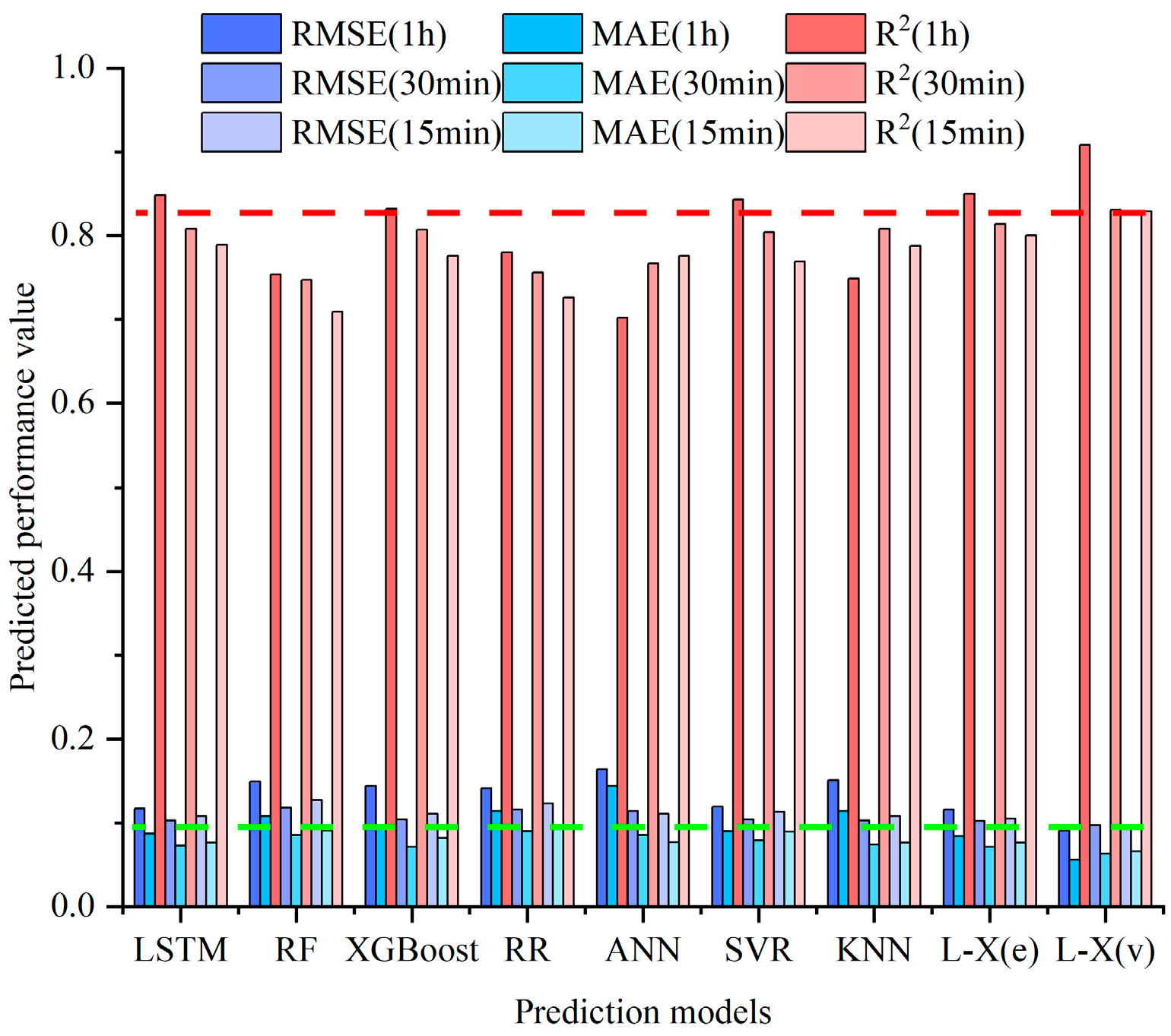
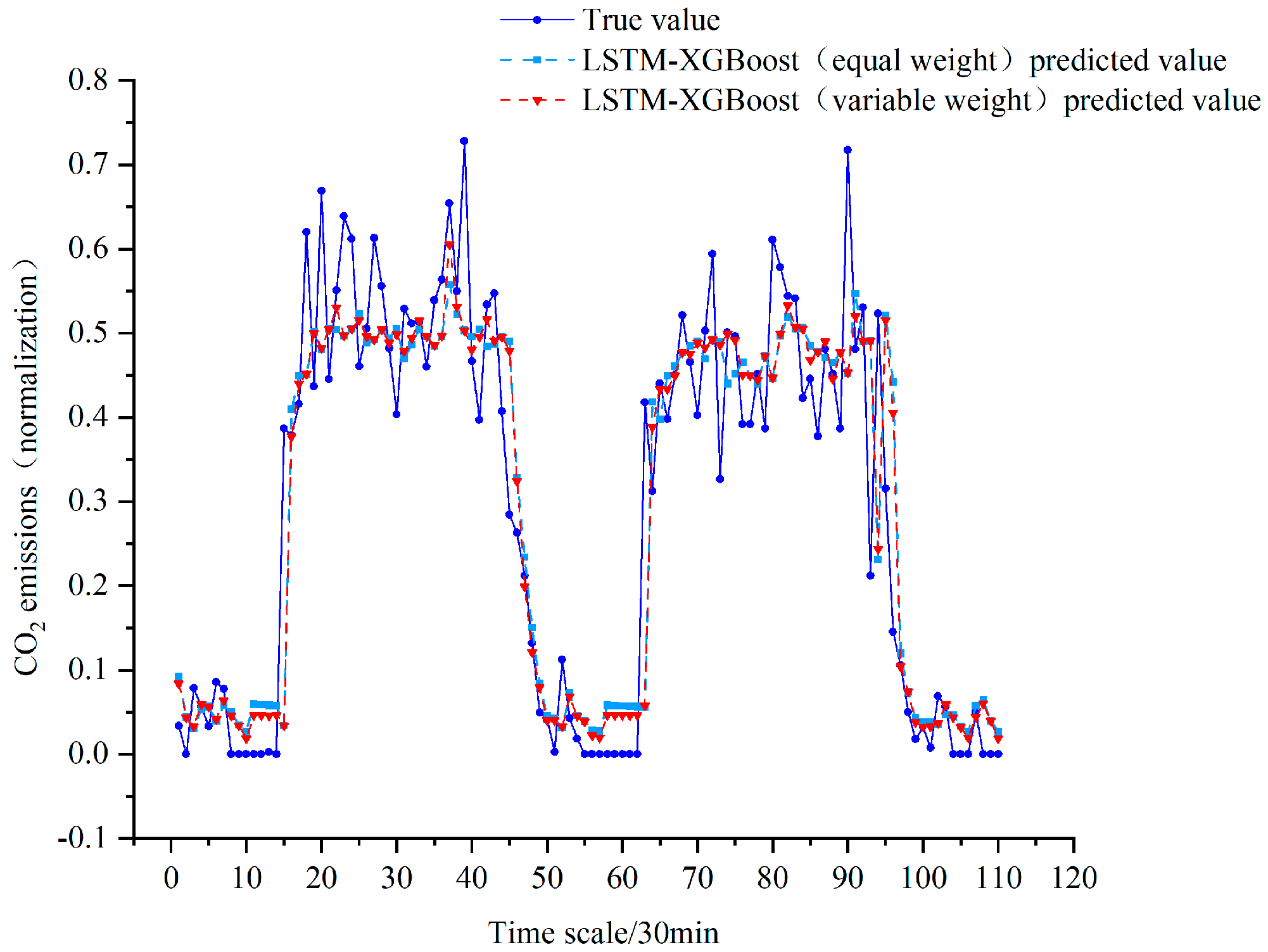
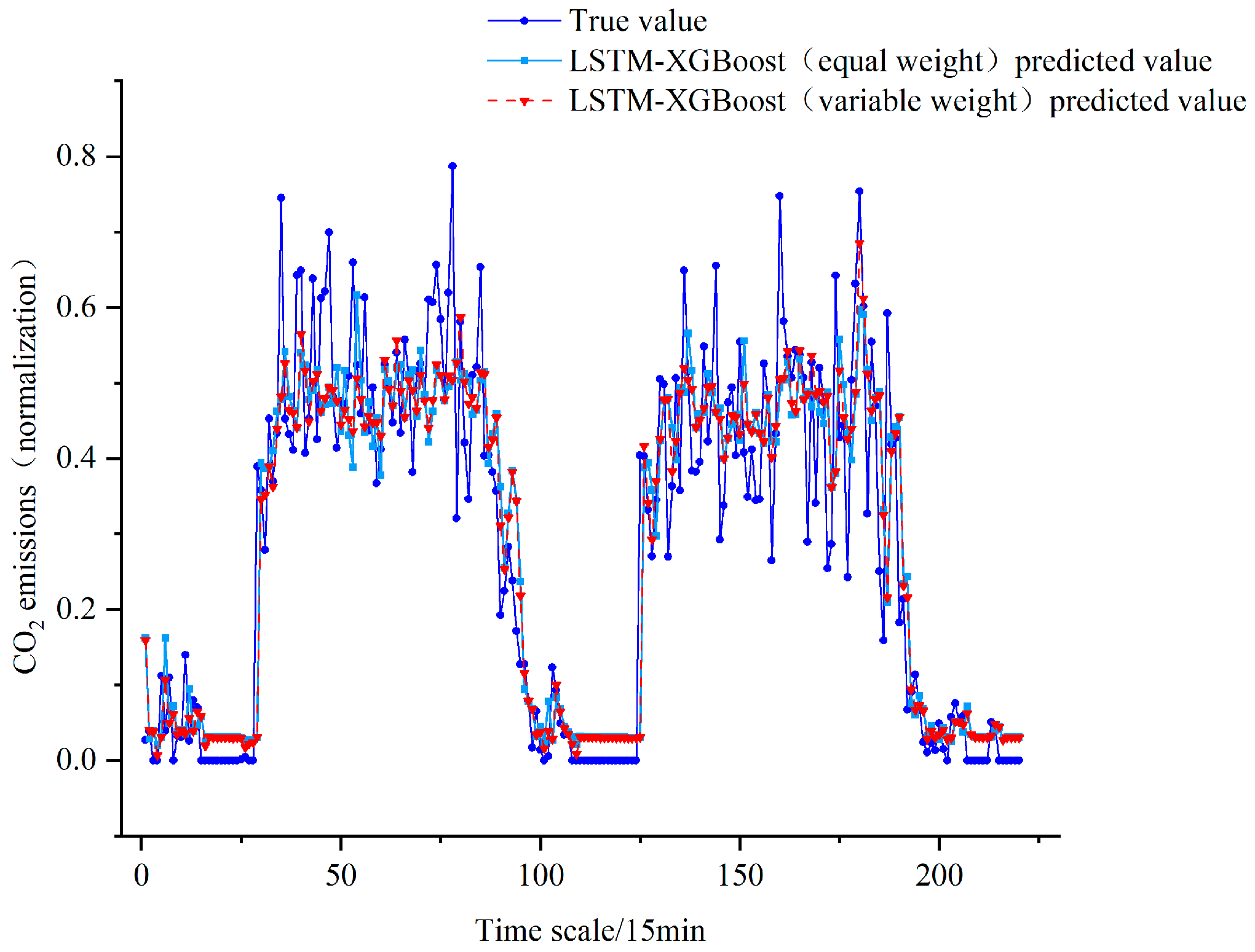
4.1. Model Prediction Results

In the process of air traffic flow management, in addition to the statistics and prediction of hourly flight flow, it is necessary to calculate the 30 min and 15 min flow in the airspace. Therefore, selecting three statistical scales of 1 h, 30 min, and 15 min in the prediction process can further test the generalization ability of the prediction model under different time granularity datasets. Considering the high proportion of CO₂ emissions in the airspace, which is much larger than other pollutants, and that the change trend of the emissions of the five pollutants is essentially the same, CO₂ is used here as an example to illustrate the prediction performance of the prediction model at different time scales. At the same time, considering the large amount of CO₂ emission data, the prediction performance parameters of the model are described with normalized data below.

In order to show the prediction advantages of the combined prediction model established in this paper, another seven single machine learning models were selected for comparison with the equal weight combined prediction model. The single machine learning models include the RF, ridge regression model (RR), ANN, SVR, k-nearest neighbor (KNN), LSTM, and XGBoost models. The results of the comparison and analysis of the prediction performance of each prediction model on three statistical scales are shown in

Table 3. Comparative results of prediction performance of different prediction models.

Prediction Models	1 h			30 min			15 min
	RMSE	MAE	R2	RMSE	MAE	R2	RMSE	MAE	R2
LSTM	0.117	0.087	0.848	0.103	0.073	0.808	0.108	0.076	0.789
XGBoost	0.144	0.092	0.832	0.104	0.074	0.807	0.111	0.082	0.776
RF	0.149	0.108	0.754	0.118	0.085	0.747	0.127	0.091	0.709
RR	0.141	0.114	0.78	0.116	0.09	0.756	0.123	0.094	0.726
ANN	0.164	0.144	0.702	0.114	0.085	0.767	0.111	0.077	0.776
SVR	0.119	0.090	0.843	0.104	0.079	0.804	0.113	0.089	0.769
KNN	0.151	0.114	0.749	0.103	0.074	0.808	0.108	0.076	0.788
LSTM-XGBoost (equal weight)	0.116	0.084	0.850	0.102	0.071	0.814	0.105	0.076	0.800
LSTM-XGBoos (variable weight)	0.091	0.056	0.908	0.097	0.063	0.831	0.097	0.066	0.829

.

Figure 10 shows the comparison chart of prediction performance of different models. The red dotted line represents the reference line of the positive performance index and the green dotted line represents the reference line of the negative performance index.

It can be seen that the LSTM prediction model and XGBoost prediction model had the best prediction performance of the single machine learning models, which confirms the rationality of using the LSTM model and XGBoost models to predict airspace flight emissions in the short term. The prediction performance of the combined prediction model was better than that of any single machine learning model, and the generalization performance of the LSTM–XGBoost (variable weight) combined prediction model (L-X (v) in Figure 10) was better than that of the LSTM–XGBoost (equal weight) combined prediction model (L-X (e) in Figure 10), showing the highest R² and the lowest RMSE and MAE in all three prediction time scales of 1 h, 30 min, and 15 min.

On the 1 h statistical scale, compared with the single machine learning model with the best prediction performance (LSTM), the LSTM–XGBoost (variable weight) combination prediction model increased R² by 7.1%, decreased RMSE by 22.2%, and decreased MAE by 35.7%. On the 30 min statistical scale, R² increased by 2.8%, RMSE decreased by 5.8%, and MAE decreased by 13.7%. On the 15 min statistical scale, R² increased by 5.1%, RMSE decreased by 10.1%, and MAE decreased by 13.2%. It can be seen that the LSTM–XGBoost (variable weight) combination prediction model established in this paper has excellent short-term prediction performance for airspace flight emissions.

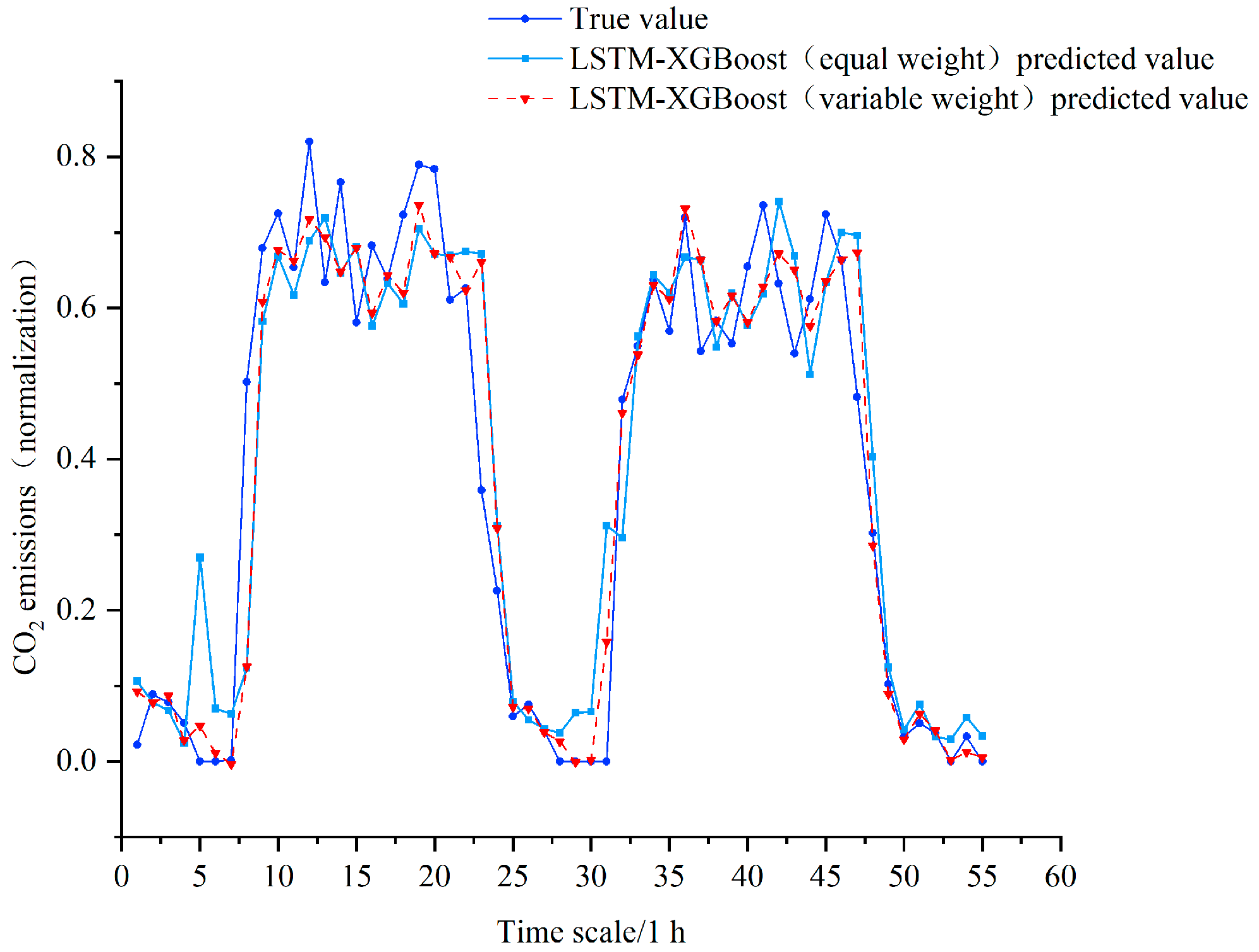
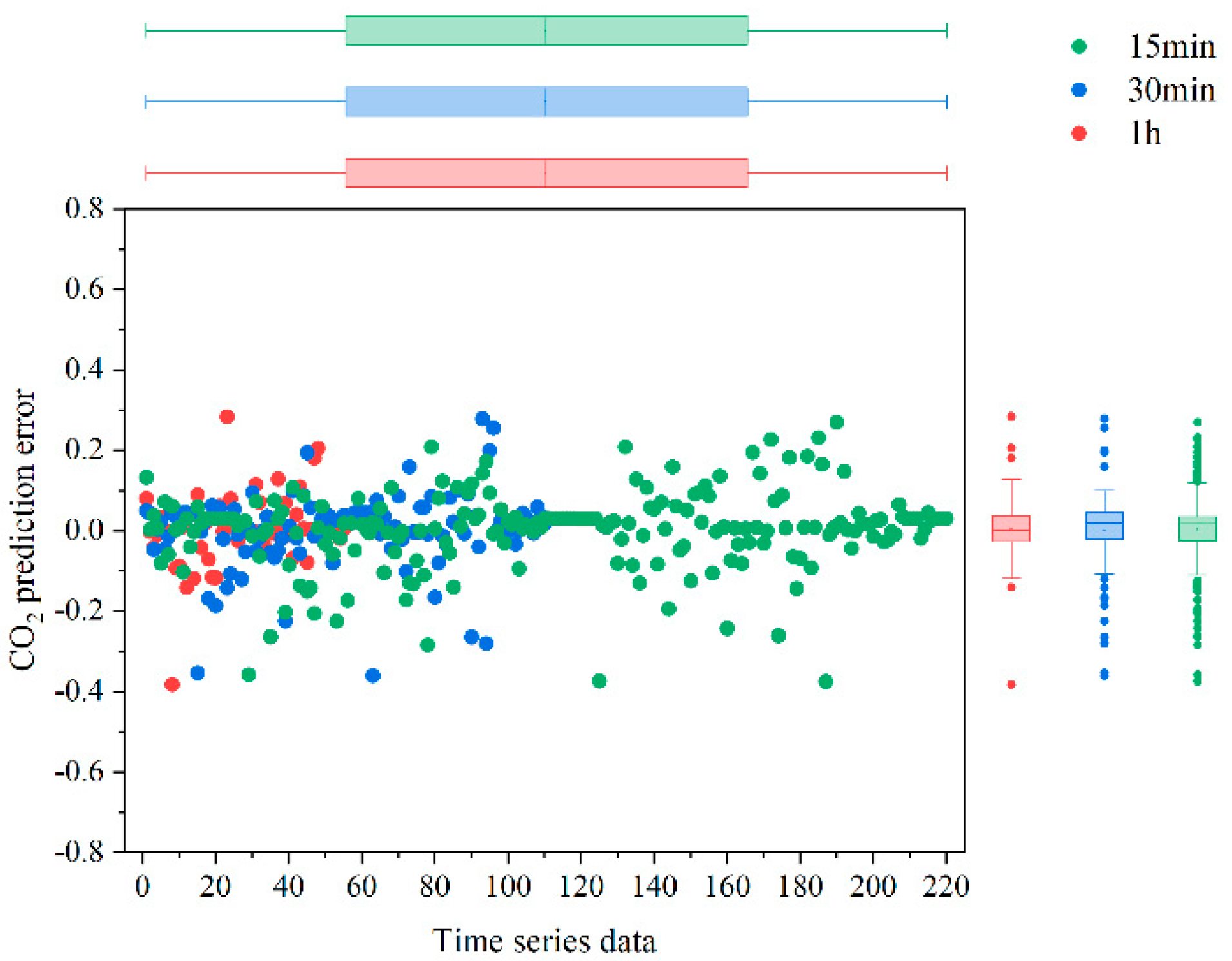
4.2. Comparison of Prediction Results

In order to further compare the predicted values and true values of the LSTM–XGBoost (variable weight) combined prediction model at the three statistical scales of 1 h, 30 min, and 15 min, the LSTM–XGBoost (equal weight) combined prediction model was taken as a reference; a broken line diagram of the predicted value and true value of the two combined prediction models is shown in Figure 11, Figure 12 and Figure 13.

According to Figure 11, Figure 12 and Figure 13, it can be seen that the LSTM–XGBoost (variable weight) combination prediction model has better results than the LSTM–XGBoost (equal weight) prediction model. Among the three statistical time scales, the prediction performance at the 1 h scale was the best. When the statistical scale is refined, the prediction performance of the model decays, which is related to the peak value of the data.

As shown in Figure 14, in order to better reveal the short-term prediction performance of the LSTM–XGBoost (variable weight) combined prediction model in airspace flight emissions, the error statistics between the prediction results and the true value were determined, taking CO₂ as an example. The mean value of the emissions prediction error on the three statistical time scales is near zero, the prediction error is relatively balanced on the larger time statistical scale, and the overall prediction performance of the model is good, which further confirms the accuracy of the model.

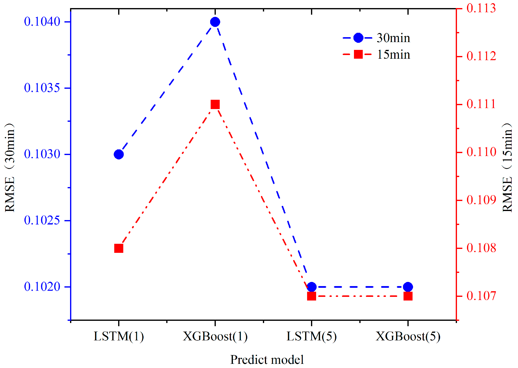
4.3. Prediction Results for Different Emissions

In order to analyze the generalization performance of the LSTM–XGBoost (variable weight) combined prediction model on the five emission data sets, the prediction of the five emissions on the three statistical time scales was predicted using the LSTM–XGBoost (variable weight) combined prediction model and the fitting curve between the predicted value and the true value was drawn.

According to Figure 15, the prediction performance of LSTM–XGBoost (variable weight) combined prediction model shows differences when using different datasets and time scales. The order of the best prediction performance for the five emissions was CO₂ > SO_X > NOx > CO > HC. This order of prediction performance is consistent with the order of emissions, showing that the prediction performance is better with larger amounts of emissions. As CO₂ and SO_X emissions are linear with fuel consumption, the respective R² of their fitting curves on the three statistical scales both exceed 0.8. The prediction fitting line R² of CO and HC on the hourly statistical scale is 0.8298 and 0.8309, respectively. The prediction performance is good, although slightly worse on the 30 min and 15 min statistical scale datasets; fortunately, R² is greater than 0.6, which is related to more zero values in the data set. By time scale, the predicted R² of the five emissions on the 1 h scale is more than 0.8, showing good prediction performance. With decreasing statistical particle size, the prediction performance deteriorates further; the overall order of prediction performance is 1 h > 30 min > 15 min.

4.4. Analysis of Factors Related to Emissions Prediction

According to the time-series diagram of the emissions of the five pollutants, it can be seen that the data show good periodicity and similar fluctuation trends, as shown in Figure 16. Through correlation analysis, it was found that the time-series correlation of the emissions of the five pollutants is good; considering this, the correlation information between emission data may provide a good auxiliary role in the prediction process. The design comparison experiment was as follows: LSTM and XGBoost single machine learning models were used to train the time series data of five kinds of emissions using two statistical scale data sets of 30 min and 15 min with slightly poor prediction performance, then testing the CO₂ emissions prediction results. The results show that the model trained with time-series data composed of all five emissions had better prediction performance on the test set than the model trained with the single time-series data set of CO₂ emissions. The specific results are shown in

Table 4. Comparative experimental results.

Data Sets	Comparative Mode	30 min			15 min
		RMSE	MAE	R2	RMSE	MAE	R2
Excluding other emissions	LSTM (1)	0.103	0.073	0.808	0.108	0.076	0.789
	XGBoost (1)	0.104	0.074	0.807	0.111	0.082	0.776
Including other emissions	LSTM (5)	0.102	0.072	0.812	0.107	0.075	0.792
	XGBoost (5)	0.102	0.070	0.814	0.107	0.075	0.795

.

LSTM (1) and XGBoost (1) in the table indicate that the training set contained only one emission characteristic of CO₂ and no other emissions, while LSTM (5) and XGBoost (5) indicate that the training set contained five emission characteristics. The comparative results of prediction performance are shown in Figure 17, Figure 18 and Figure 19. Compared with the model trained with all five emissions, the RMSE and MAE of the model trained with a single emission are smaller and the R² is larger. At the same time, it can be seen that the prediction model trained with the 30 min statistical scale dataset shows smaller RMSE and MAE and a larger R² compared with the prediction model trained with the 15 min statistical scale dataset.

5. Conclusions

In this paper, we established a short-term prediction model of airspace flight emissions integrating the LSTM network and XGBoost model. According to the experimental results, the following conclusions can be drawn:

(1)

The time-series information of emissions from airspace flights have good periodic characteristics, and it is feasible and effective to forecast short-term emissions.

(2)

In the single machine learning model, the short-term prediction ability of airspace flight emissions using the LSTM network and XGBoost models is better than the other single machine learning models, and the variable weight combination prediction model has better prediction robustness than the equal weight combination prediction model.

(3)

The adaptive time-varying weighting model combining LSTM network and XGBoost model considers both the time series characteristics of data, takes into account the nonlinear characteristics of data, and can correct the prediction error of a single prediction model. The prediction accuracy is generally good, and the prediction performance of the model decreases with the statistical time scale.

(4)

In the process of prediction, similarity information transfer occurs between different emissions, and multi-feature factors can be used to train the prediction model to improve its prediction ability.

(5)

This paper is a theoretical exploration of the short-term prediction of airspace flight emissions. In the future, we can comprehensively consider the traffic information parameters of airspace and parallelize the airspace data in combination with airspace big data monitoring platforms to improve the prediction accuracy and stability of the model. This is an important research direction for taking the next step in combining the time series information of emissions in multi-sector airspace to study the temporal and spatial variation of emissions in different regions and further the intelligent perception of airspace operation quality.

References

- International Air Transport Association (IATA). 20 Year Passenger Forecast 2014–2034; International Air Transport Association: Montreal, QC, Canada, 2014. [Google Scholar]
- International Civil Aviation Organization (ICAO). 2019 Environmental Report: Aviation and Environment; International Civil Aviation Organization: Montreal, QC, Canada, 2019. [Google Scholar]
- Liu, F.Z.; Li, Z.H.; Xie, H.; Yang, L.; Hu, M.H. Predicting fuel consumption reduction potentials based on 4D trajectory optimization with heterogeneous Constraints. Sustainability 2021, 13, 7043. [Google Scholar] [CrossRef]
- Wei, Z.Q.; Zhang, W.X.; Han, B. Optimization method of aircraft cruise performance parameters considering pollution emissions. Acta Aeronaut. Astronaut. Sin. 2016, 37, 3485–3493. [Google Scholar]
- Turgut, E.T.; Cavcar, M.; Usanmaz, O. Investigating actual landing and takeoff operations for time-in-mode, fuel and emissions parameters on domestic routes in Turkey. Transp. Res. Part D Transp. Environ. 2017, 53, 249–262. [Google Scholar] [CrossRef]
- Li, J.; Zhao, Z.Q.; Liu, X.G. Study an analysis of aircraft emission inventory for Beijing capital International airport. Chin. Environ. Sci. 2018, 38, 4469–4475. [Google Scholar]
- Li, N.; Zhang, H.F. Calculating aircraft pollutant emissions during taxiing at the airport. Acta Sci. Circumst. 2017, 37, 1872–1876. [Google Scholar]
- Cao, H.L.; Tang, X.H.; Miao, J.H. Calculation and analysis of nitrogen oxide emission in LTO stage of engine basedon QAR data. Acta Sci. Circumst. 2018, 38, 3900–3904. [Google Scholar]
- Yu, N.; Zhang, M.Y.; Zhang, Y.; Tian, Y.; Zeng, R.M. Aircraft cruising phase airborne pollutant emission and dispersion. Sci. Technol. Eng. 2020, 20, 28281–28285. [Google Scholar]
- Han, B.; Liu, Y.T.; Tan, H.Z.; Wang, Y.; Wei, Z.Q. Emission characterization of civil aviation aircraft during a whole flight. Acta Sci. Circumst. 2017, 37, 4492–4502. [Google Scholar]
- Gao, L. Study on the Assessment Method of Airport Environment Carrying Capacity; Nanjing University of Aeronautics and Astronautics: Nanjing, China, 2019; pp. 54–55. [Google Scholar]
- Yang, R. Analysis and Control Strategy of Airport Ground Taxiing for Energy Saving and Emission Reduction; Civil Aviation University of China: Tianjin, China, 2019; pp. 41–43. [Google Scholar]
- Yang, L.; Li, W.B.; Liu, F.Z.; Chen, Y.T.; Zhao, Z. Multi-objective optimization of continuous descending trajectory in flexible airspace. Acta Aeronaut. Astronaut. Sin. 2021, 42, 206–222. [Google Scholar]
- Chen, D.; Hu, M.H.; Han, K.; Zhang, H.H.; Yin, J.N. Short/medium-term prediction for the aviation emissions in the en-route airspace considering the fluctuation in air traffic demand. Transp. Res. Part D Transp. Environ. 2016, 48, 46–62. [Google Scholar] [CrossRef]
- Chen, D. Research on the Methods of En Route Traffic Flow Management Based on Network Traffic Demand Prediction; Nanjing University of Aeronautics and Astronautics: Nanjing, China, 2018; pp. 65–78. [Google Scholar]
- Li, C. Research on Aviation Emission Analysis and Forecasting Methods; Nanjing University of Aeronautics and Astronautics: Nanjing, China, 2020; pp. 58–67. [Google Scholar]
- Lee, S.D.; Fahey, D.W.; Forster, P.M.; Newton, P.J.; Wit, R.C.N.; Ling, L.L.; Owen, B.; Sausen, R. Aviation and global climate change in the 21st century. Atmos. Environ. 2009, 43, 3520–3537. [Google Scholar] [CrossRef] [PubMed] [Green Version]
- Wuebbles, D.; Forster, P.; Rogers, H.; Herman, R. Issues and uncertainties affecting metrics for aviation impacts on climate. Bull. Am. Meteorol. Soc. 2010, 91, 491–496. [Google Scholar] [CrossRef] [Green Version]
- Pejovic, T.; Noland, R.B.; Williams, V.; Toumi, R. Estimates of UK CO2 emissons from aviation using air traffic data. Clim. Chang. 2008, 88, 367–384. [Google Scholar] [CrossRef]
- EUROCONTROL. User Manual for the Base of Aircraft Data (BADA) Revision 3.11. 2019. Available online: https://www.eurocontrol.int/publication/user-manual-base-aircraft-data-bada-revision-31 (accessed on 20 March 2022).
- Yang, C.K. Arrival Efficiency Evaluation and Abnormal Status Analysis of Flights; Civil Aviation University of China: Tianjin, China, 2019; pp. 38–40. [Google Scholar]
- Guo, Y.J.; Ding, Y.H. Upper-air specific humidity change over China during 1958–2005. Chin. J. Atmos. Sci. 2014, 38, 1–12. [Google Scholar]
- Zhang, Y.; Yang, S.M.; Xin, D.R. Short-term Traffic Flow Forecast Based on Improved Wavelet Packet and Long Short-term Memory Combination Model. J. Transp. Syst. Eng. Inf. Technol. 2020, 20, 204–210. [Google Scholar]
- Fan, Z.Z.; Zhao, Y.; Zhou, N.; Zhao, C.; Zhang, W.Y. Integrated model for forecasting waterway traffic accidents based on the Gray-BP neural network. J. Saf. Environ. 2020, 20, 857–861. [Google Scholar]
- Xie, X.B.; Kong, L.Y. On the ways to the traffic accident prediction based on the ARIMA and XGBoost combined model. J. Saf. Environ. 2021, 21, 277–284. [Google Scholar]
- Wang, S.; Wei, L.F.; Zeng, L. A Combined Model for Photovoltaic Power Forecasting Based on GWO-SVM and Random Forest. J. Kunming Univ. Sci. Technol. 2021, 46, 1–8. [Google Scholar] [CrossRef]
- Li, L.; Zhang, Q.M.; Zhao, J.H.; Nie, Y.W. Short-Term Traffic Flow Prediction Method of Different Periods Based on Improved CNN-LSTM. J. Appl. Sci. 2021, 39, 185–198. [Google Scholar]
- Chen, Z.Y.; Liu, J.B.; Li, C.; Ji, X.H.; Li, D.P.; Huang, Y.H.; Di, F.C.; Gao, X.Y.; Xu, L.Z. Ultra Short-term Power Load Forecasting Based on Combined LSTM-XGBoost Model. Power Syst. Technol. 2020, 44, 614–620. [Google Scholar]
- Bai, S.N.; Shen, X.L. PM2.5 Prediction based on LSTM recurrent neural network. Comput. Appl. Soft. 2019, 36, 67–70, 104. [Google Scholar]
- Zhong, Y.; Shao, Y.M.; Wu, W.W.; Hu, G.X. Short-term traffic flow prediction model based on XGBoost. Sci. Technol. Eng. 2019, 19, 337–342. [Google Scholar]
- Tan, M.M. Short Term Traffic Flow Forecasting Based on Integration of LSTM Model and Grey Model; Nanjing University of Posts and Telecommunications: Nanjing, China, 2017; pp. 18–36. [Google Scholar]
- Pan, B. Application of XGBoost algorithm in hourly PM2.5 concentration prediction. IOP Conf. Ser. Earth Environ. Sci. 2018, 113, 012127. [Google Scholar] [CrossRef] [Green Version]
- Qu, J.; Chen, H.Y.; Liu, W.Z.; Li, Z.B.; Zhang, B.; Ying, Y.H. Application of Support Vector Machine Based on Improved Grid Search in Quantitative Analysis of Gas. Chin. J. Sens. Actuators 2015, 28, 774–778. [Google Scholar]