Article

A Framework-Based Wind Forecasting to Assess Wind Potential with Improved Grey Wolf Optimization and Support Vector Regression

1
Department of Electrical and Electronics Engineering, College of Engineering Guindy, Anna University, Chennai 600025, India
2
Department of Electrical and Electronics Engineering, Sri Venkateswara College of Engineering, Chennai 602117, India
3
Discipline of Engineering and Energy, Murdoch University, Murdoch, WA 6150, Australia
*
Authors to whom correspondence should be addressed.
Sustainability 2022, 14(7), 4235; https://doi.org/10.3390/su14074235
Submission received: 16 February 2022 / Revised: 28 March 2022 / Accepted: 29 March 2022 / Published: 2 April 2022

Abstract

:
Wind energy is one of the most promising alternates of fossil fuels because of its abundant availability, low cost, and pollution-free attributes. Wind potential estimation, wind forecasting, and effective wind-energy management are the critical factors in planning and managing wind farms connected to wind-pooling substations. Hence, this study proposes a hybrid framework-based approach for wind-resource estimation and forecasting, namely IGWO-SVR (improved grey wolf optimization method (IGWO)-support vector regression (SVR)) for a real-time power pooling substation. The wind resource assessment and behavioral wind analysis has been carried out with the proposed IGWO-SVR optimization method for hourly, daily, monthly, and annual cases using 40 years of ERA (European Center for Medium-Range Weather Forecast reanalysis) data along with the impact of the El Niño effect. First, wind reassessment is carried out considering the impact of El Niño, wind speed, power, pressure, and temperature of the selected site Radhapuram substation in Tamilnadu, India and reported extensively. In addition, statistical analysis and wind distribution fitting are performed to demonstrate the seasonal effect. Then the proposed model is adopted for wind speed forecasting based on the dataset. From the results, the proposed model offered the best assessment report and predicted the wind behavior with greater accuracy using evaluation metrics, namely root mean square error (RMSE), mean absolute error (MAE), and mean squared error (MSE). For short-term wind speed, power, and El Niño forecasting, IGWO-SVR optimization effectively outperforms other existing models. This method can be adapted effectively in any potential locations for wind resource assessment and forecasting needs for better renewable energy management by power utilities.

1. Introduction

1.1. Background

Rapid economic growth needs an increase in energy production that should be cost-effective and pollution-free [1,2,3]. Renewable energy, particularly wind and solar, is coming into the limelight because of its advantages, such as being cost-effective and non-pollutant, and the abundant fuel from nature compared with fossil fuels and gas fuels [4,5,6]. A total of 195 members of the UN Framework of Climate Change (UNFCCC) contracted an assurance to attain renewables as of November 2019 [7]. As per Pari’s Commitment to promoting green energy worldwide, India committed to building 175 GW capacity in 2022 [8], wherein 100 GW is wind installed capacity [9]. India has a wind onshore installed capacity of 38.789 GW and is exploring offshore wind in the coastal areas of Tamilnadu. It has abundant renewable energy resources with a wind installed capacity of 9231.77 MW and a solar installed capacity of 4500 MW [10], catering to leading industrialization growth in India. Tamilnadu has about 9500 wind turbines distributed in 125 wind pooling substations [11].
Wind energy is stochastic because of climatic changes like the El Niño effect, and hence wind energy patterns need to be continuously assessed. However, detecting the pattern and forecasting wind behavior plays a significant part in determining wind energy potential [12,13]. Proper wind speed and power forecasting are also assessed for better renewable energy management in the load dispatch center (LDC). In addition, wind energy management in the LDC depends on wind data information from wind pooling substations. To handle renewable energy management across the state, attempts at micro wind energy management at wind pooling substations by conducting wind behavioral studies and wind forecasting methods are carried out. Many authors reported many probabilistic frequency distributions to model the wind speed. Nevertheless, these works have a few drawbacks, i.e., they failed to adjust in the wind distribution fitting histogram. At present, the use of intelligence practices is adapted to optimize the parameters that minimize the inaccuracies in energy production. Researchers rarely use hybrid optimizations to obtain the most optimal solutions. Therefore, it is essential to implement the most optimized intelligence techniques to assess and forecast wind potential for any site.

1.2. Literature Survey

Considering the above needs, this section provides a robust literature survey relating to the potential assessment and forecasting. There are significant works available from different sources with possible outcomes, and a few of them are described in Table 1.
Considering all the above inferences, a research gap was found in improving wind forecasting accuracy using a hybrid optimization model. Most of the existing research demonstrated the assessment of wind farms without significant illustration of wind forecasting. Also, El Niño effects are not considered for wind parameter assessment and forecasting. Moreover, most of the wind energy farms were commissioned a few years ago and their existing potential assessment reports are outdated, as the recent sophisticated assessment approaches offer more precise values. In addition, the considered Radhapuram pooling station is ready for re-powering with advanced wind turbines. Therefore, this study focuses on reassessing and forecasting wind energy potential with the improved grey wolf optimization-support vector regressions (IGWO-SVR) method using 40 years of ERA (European Center for Medium-Range Weather Forecast reanalysis) data. ERA provides current forecasts, climate re-analyses, and specific datasets that are available via the web, point-to-point dissemination, data servers, and broadcasting data. The short-term wind forecasting is carried out for wind speed, wind power, and El Niño scheduling and trading with the SVR method optimized by the IGWO technique. Therefore, this study developed an advanced optimization technique for wind energy management in the Radhapuram 110/33-11 kV wind pooling substation in Tamilnadu. The substation connected with 136 MW installed wind turbines spanned in 15 incoming feeders and five different makes of wind turbines with various capacities. It is essential to reassess the wind potential of the selected site to identify the effects of El Niño. This study will be a useful tool for the power utilities, government agencies, and researchers for future decision-making over installing similar wind power plants.

2. Wind Energy Management in Pooling Substation

Wind Energy is stochastic in nature and any location with wind speed and direction, depending on climatic and seasonal changes. The wind characteristics change by the day, season, and year, and are subject to the recent focus on El Niño’s impact on climatic conditions. The wind energy management in the Radhapuram substation is categorized in this paper, with wind potential reassessment over 40 years of ERA data with wind distribution methods through parameter estimation.

2.1. Wind Pattern Analysis

Lidar and sodar, metrological instruments, are mounted in tall towers to estimate the wind parameters at the ground level. Both instruments play a crucial role in the primary data collection of wind resource valuations. The key parameters of all wind-observing suites are wind pressure, wind speed, wind direction, and temperature. Commonly, the following parameters are measured for specific applications:
-
To ensure wind suitability evaluation and wind turbine selection, maximum, minimum, and average wind speed, and standard deviation are assessed;
-
To comprehend the wind distribution and optimized micro siting of wind turbines, the highest gust direction and standard deviation are computed;
-
Turbulence intensity and wind density are evaluated using the observed temperature and wind speed (vertical);
-
For atmospheric assessment and icing effect in the site, the average, minimum and maximum value of solar irradiation and relative humidity (%) are estimated.
For long-term wind resource assessment studies, nearby station data or airport data can be used. Satellite data from MERRA and ERA can also be used for in-depth wind resource studies. Recent studies like El Niño’s impact on climatic changes, which indirectly impact wind flow variations, can also be taken in this research analysis.

2.2. Wind Speed Distribution Models

Wind distribution configuration is crucial for wind information, which is assessed by the mean wind speed and percentage of occurrences at hub height of 100 m. This information helps to evaluate the output power of the turbine system unswervingly. The incidence of wind distribution signifies the figure of interims in the course of the data collection during the falling of wind speed inside an actual bin; this typically happens around 0.5 or 1.0 m/s and manages the lowest speed ranges labeled for the power curve of the chosen turbine notably from 0 to 25 m/s. Furthermore, wind forecasting is a mathematical design to visualize the pattern of the wind speed, wind power, and the El Niño effect, but they are not stable because of atmospheric changes that happen relentlessly. It is known that wind power generation is the task of wind speed and its density, and therefore it is essential to perform wind speed prediction. Table 2 illustrates several real-time data patterns with their required ranges.

2.3. Performance Metrics Analysis

The performance metrics signify the best fit for a forecasting study and match actual measured values with greater accuracy. In this work, four metrics are considered to study the precision of the forecasted wind data assessment: mean absolute error (MAE), root mean square error (RMSE), and mean squared error (MSE). The best-scored RMSE, MAE, and MSE [26,27,28] provide the best-fitted wind distribution process for the definite sites.

2.3.1. Mean Absolute Error (MAE)

M A E = 1 N i = 1 N | A i P i |
where Ai and Pi are measured and predicted values, respectively, and N is the number of observations.

2.3.2. Root Mean Squared Error (RMSE)

This estimates the residuals of the probability density function occurrence and the measured data.
R M S E = [ 1 n i = 1 n ( y i x i ) 2 ] 0 , 5  
where yi denotes the perceived statistics schemed in a histogram, n terms the number of bins, and xi signifies the projected PDF function of wind distribution pattern taken for assessment. Its range should be close to zero to ensure the goodness of fit.

2.3.3. Mean Squared Error (MSE)

M S E = 1 N i = 1 N ( Y i Y ^ l ) 2

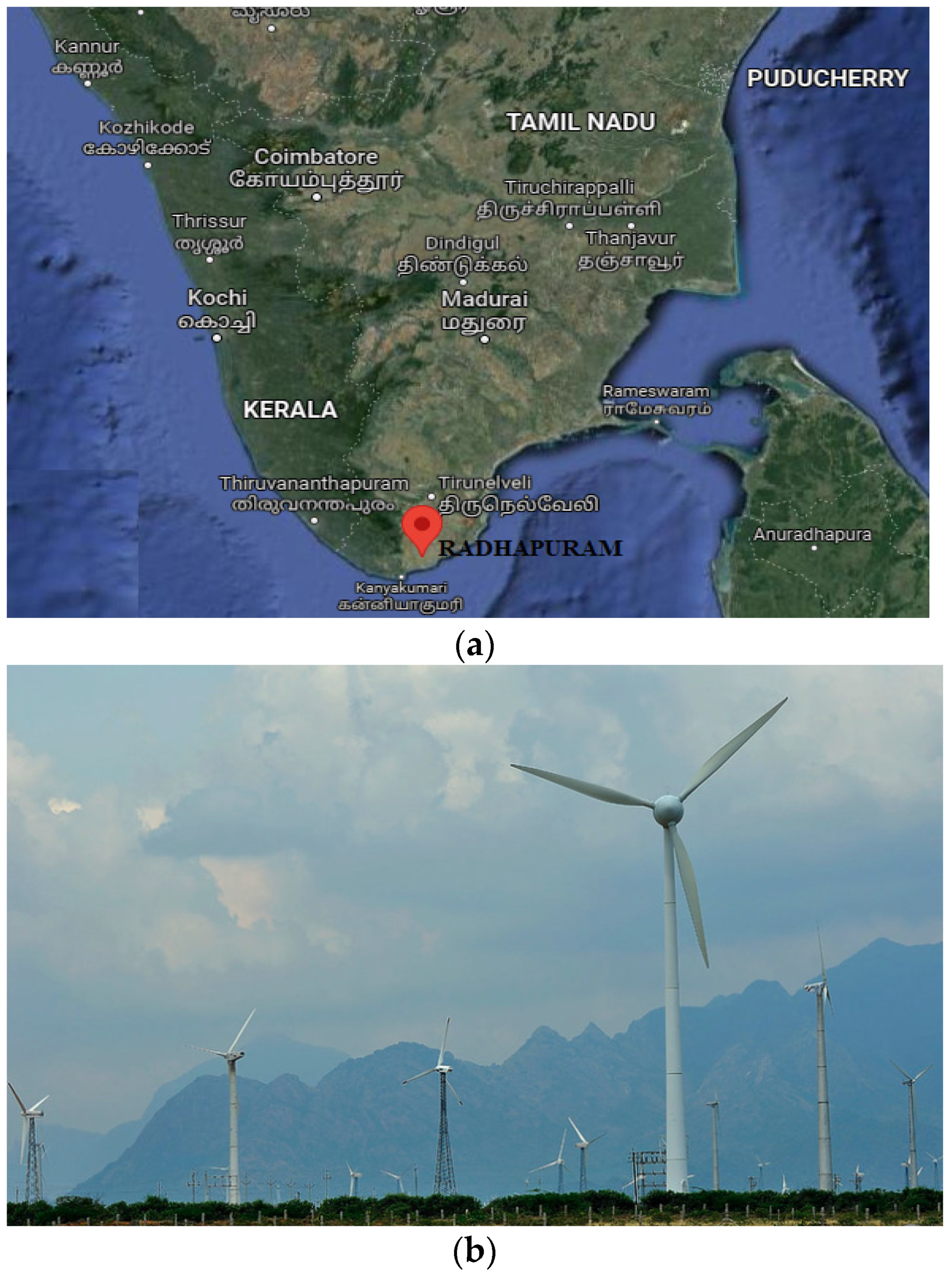
3. Case Study and Its Descriptions

The wind data are analyzed from the ERA web portal for Radhapuram wind pooling station, 110/33-11 kV substation, Tamilnadu. The wind pooling station evacuates wind energy to the upstream Sanganeri 230 kV grid substation. The Radhapuram wind pooling station handles 15 wind pooling feeders, 101 wind turbines spanned to 15 wind feeders with a maximum aggregated wind installed capacity of 136 MW. The statistics of the substation location are presented in Table 3, and the mapping and site of the selected area are illustrated in Figure 1.

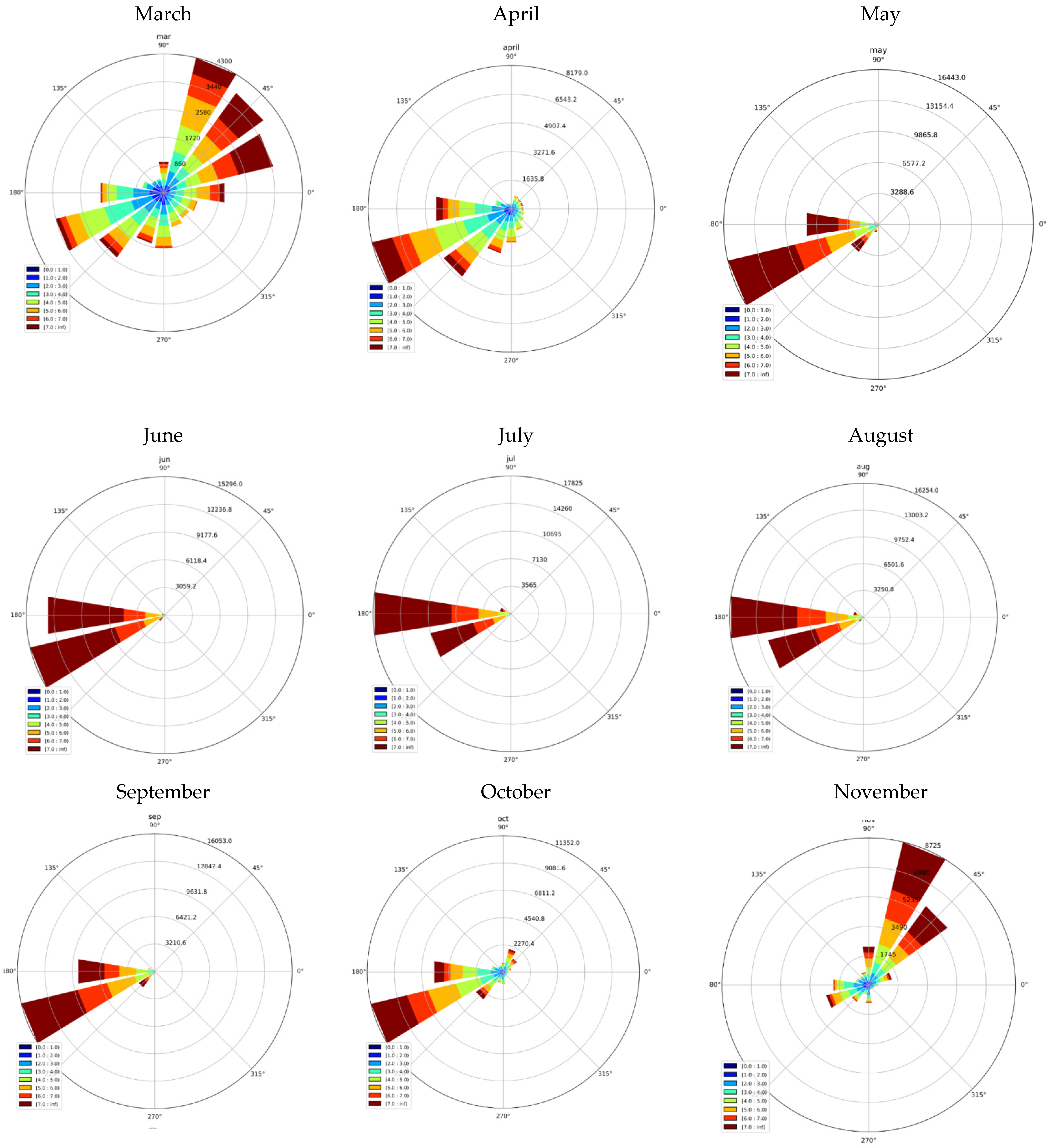
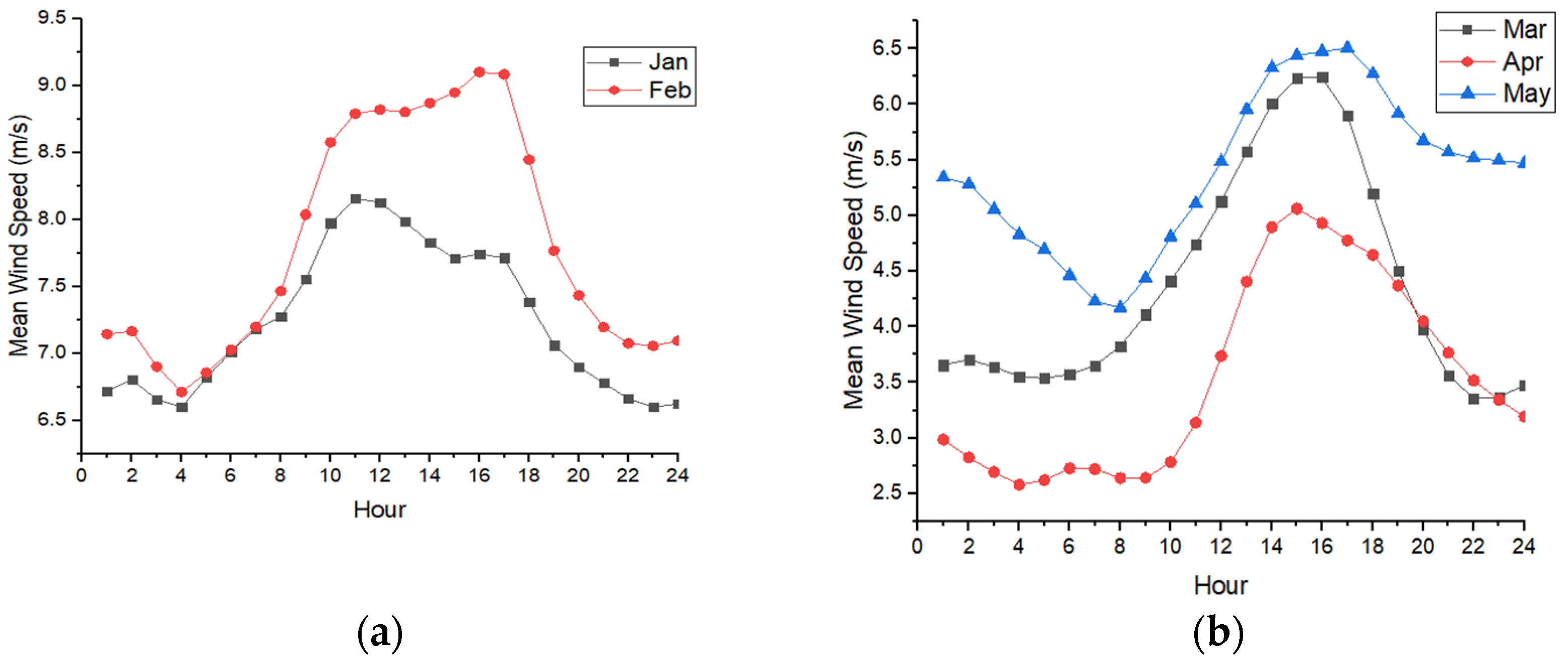
3.1. Wind Seasonal Pattern

Among the Indian states, two central states, Tamilnadu [29] and Gujarat [30], have maximum wind power potential. For both states, monsoon seasons are classified into four periods, such as northeast monsoon (NEM), southwest monsoon (SWM), summer, and winter, and considered for this study [31]. These monsoon periods are clustered based on wind speed and months, as given in Table 4.

3.2. Wind Power Density (WPD)
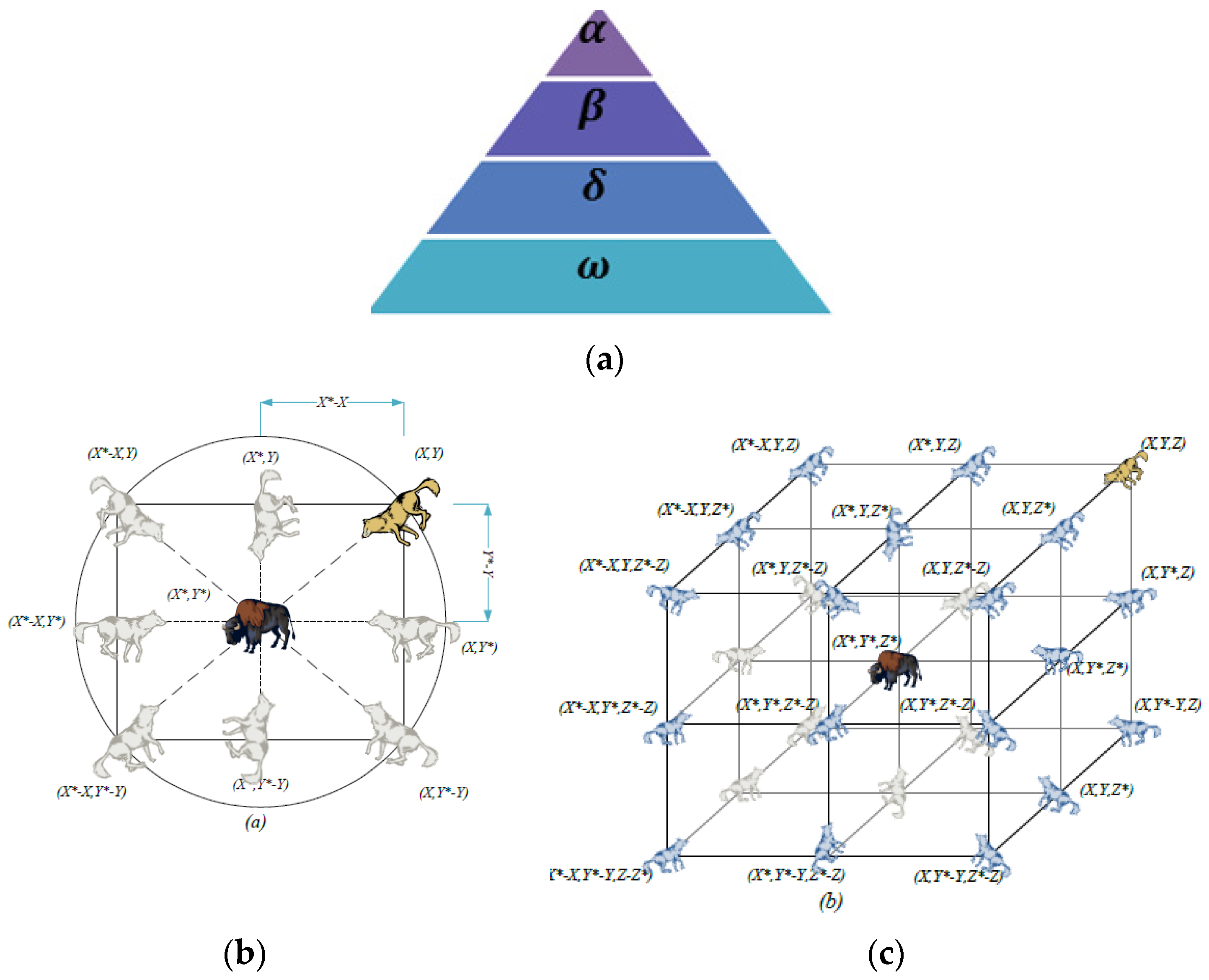
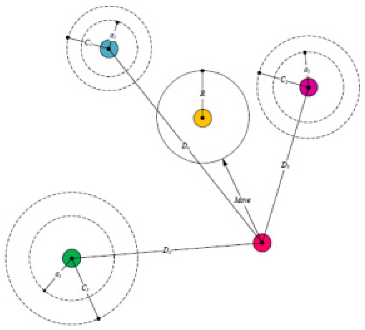
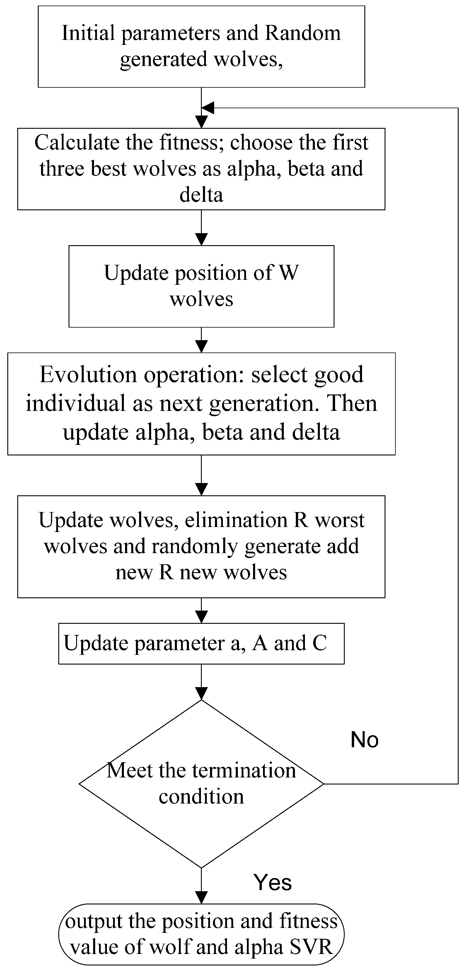
WPD modeling provides detailed information of wind energy distributions for various wind speed magnitudes; notably, it varies with the cube of wind speed. The range of WPD is the chief influence for potential wind valuation in a selected site. It aids in estimating economic viability before implementing the wind farm. It can be computed using the following equations:
P w d = P A = 1 2 ρ v 3
where P and A represent the wind power (watts) and swept area (m2), respectively. ρ and v signify the air density (kg/m3) and wind speed (m/s), respectively. Taking account of the wind speed distribution, WPD can be stated as follows [25]:
      p A = 1 2 ρ 0 v 3 f ( v ) d v
To evaluate the WPD of a specific distribution, the WPD distribution function f(v) is considered and derived as follows:
Wind   power   P = 1 2 ρ A v 3 f ( v )
P A = 1 2 ρ v 3 f ( v )
Finally, the goodness of fit for WPD can be computed using below equation:
      e W P D = ( ( W P D o W P D e c ) W P D o ) 100 %
where   W P D o , the detected WPD, and WPDec are the computed scales from distribution fitting, and   W P D o signifies the error between detected and computed values.

4. Methodology

To increase the performance of the GWO, the conventional technique is classified into two perceptions: dynamic subjective approach and nonlinear convergence for influence. The convergence aspect directly affects the IGWO parameter’s value, which declines linearly [0, 2]. While optimization takes a convergence nonlinearly, the linear convergence factor doesn’t affect the tangible searching procedure. Consequently, an innovative nonlinear convergence scheme is presented in Figure 2.
GWO is a recently proposed metaheuristic technique developed based on the grey wolves’ nature-motivated leadership grading and cluster hunting process [32,33]. This approach is an operative metaheuristic adapted for many engineering optimization processes [34]. For every iteration, a total of three best wolves are engaged from the search practice, thus providing a robust convergence headed for these wolves. However, it has drawbacks, notably because of the lack of population diversity that cause the inequity between exploration, exploitation, and premature convergence [35,36,37].
To alleviate the faintness of these GWO, an improved version is carried out and defined as an improved grey wolf optimizer (IGWO). It increases the hunting exploration approach of wolves using the dimension learning-based hunting (DLH) scheme. This DLH search scheme is stirred based on nature’s different hunting comportment of wolves. It also raises the global search adopting multi-neighbor learning. As an outcome, this advanced scheme triggers the wolves from their current position to the best position for each iteration. Additionally, this proposed modification helps select and update its current position while heading for the next iteration.
Generally, the wolves have been segregated into alpha, beta, delta, and omega groups to mimic wolves’ inner leadership grading. With these groups, first-best, second-best, and third-best individuals are logged as alpha, beta, and delta, respectively, and the remaining individuals are taken as omega. Additionally, alpha, beta, and delta guide the hunting process, and other wolves are likely in the finest region in the searching location. In the iterative searching course, the three most acceptable spaces are considered for the probable location of the prey, and the position of the prey is assessed by the alpha, beta, and delta. For optimal solution, the positions of wolves are updated with the following equation:
D > = | C > X p > ( t ) X > ( t ) |
X ( t + 1 ) > = X p > ( t ) A > D >
where the term ‘t’ denotes the tth iteration, A and C represent the vector coefficient, x signifies the prey’s location, and X symbolizes the wolf’s position. The vector coefficients are computed using the following equations:
A = 2 a , r i a
C = 2 r 2
These coefficients decline from 2 to 0 linearly with the iteration counts r1 and r2 and random vectors positioned in the scope [0, 1]. In IGWO, the α, β, and δ lead ω wolves are in the direction of the extents of the search space that are hopeful for computing the optimal solution. This characteristic can head to set up local optima solutions as shown in Figure 3. Additional problems are with the lessening of the population diversity that allows IGWO to acquire local optima. Here, IGWO is suggested to alleviate such concerns. The enhancements comprise a novel search approach related to two steps (select and update), and the same is designated below using dashed lines.
Mathematically, the position updating can be described as follows:
D i s c a l p h a = | C 1 × X a l p h a ( l ) X ( l ) | D i s c b e t a = | C 1 × X b e t a ( l ) X ( l ) | D i s c d e l t a = | C 1 × X d e l t a ( l ) X ( l ) | X 1 = X a l p h a ( l ) A 1 × D i s c a l p h a X 2 = X b e t a ( l ) A 2 × D i s c b e t a X 3 = X d e l t a ( l ) A 3 × D i s c d e l t a
X ( l + 1 ) = X 1 + X 2 + X 3 3
The following scientific formulations are employed to re-tune the locations of the omega wolves. The position of the wolves is updated based on the above-mentioned rules as equations. The figure shows that the wolf at the position (X, Y) repositions its place around the prey, rendering to the above-derived updating formulations. It is also noted that the wolf can possibly move only seven positions, but regulation of the arbitrary factors (A and C) makes the wolf reposition the situation to an incessant location near prey at any position.
V 1 = | f ( x a l p h a ) | | f ( x a l p h a ) + | f ( x b e t a ) | + | f ( x d e l t a ) | | V 2 = | f ( x b e t a ) | | f ( x a l p h a ) + | f ( x b e t a ) | + | f ( x d e l t a ) | | V 3 = | f ( x d e l t a ) | | f ( x a l p h a ) + | f ( x b e t a ) | + | f ( x d e l t a ) | |
The suggested social grading supports IGWO in saving the most significant resolutions acquired for the complete iterations. A circle-based neighborhood is formed around the solutions by the anticipated IGWO; it can also be adapted for higher spaces, namely the hypersphere. Notably, the arbitrary factors (A and C) aid the candidature results to attain hyperspheres considering diverse random radius. Additionally, it provides a space for the solutions to locate estimated location and prey using the anticipated hunting model. Meanwhile, the proposed scheme ensures exploitation and exploration using the adaptive standards (a and A). These parameters help IGWO to make a transition smoothly between exploitation and exploration. Specifically, the halves of the iterations are dedicated for exploration (|A| ≥ 1) with a diminishing of A; the remaining halves are devoted for exploitation (|A| < 1). The complete process of the method is illustrated in Figure 4.
SVR forecasts the data and endeavors to diminish the structure jeopardy [38,39,40,41,42]. For high-dimensional needs, it is possible to solve the linear regression solution employing the nonlinear transformation, which aids in mapping input parameters and more significant sizes. It diminishes the operational menace and becomes good learning and generalization capacity that can reduce the algorithm’s complexity. As well, it offers more tremendous advantages such as quick convergence and global optima [43,44,45]. Additionally, it could subjectively estimate the nonlinear functions and provide superior advantages for predicting problems.
The regression function of the SVR is:
f(x) =λT ψ(x) + γ
where λT is the transpose of the weight coefficient matrix, γ is the value of offsets, and ψ(x) is a charting function. By employing the in-sensitive loss function, the above equation can be written as follows:
min ( 1 2 | | λ 2 | | + l i = 1 p ( ξ i + ξ j ) )                 s , t ( y i λ x i γ ζ i + h λ x i + γ y i ζ j + h ζ i , ζ j 0 , i = 1 , 2 , ρ , j = 1 , 2 ρ
where λ and h are penalty items and insensitive loss function, respectively. The terms ζi, ζj denote the slack relations. Considering the Lagrange and dual theory function, it is possible to derive the regression function using the following function:
f ( x ) = i = 1 p ( α i α j ) C ( x , x i ) + γ
where alpha i and alpha j are lagrangian multipliers, and C(x, xi) signifies a kernel function and is derived using the following equation:
C ( x , x i ) = exp ( v | | x x i | | 2 ) , v > 0
In this work, forecasting based on IGWO and SVR, i.e., the IGWO-SVR method, is performed and the hybrid approaches are employed for wind speed forecast at Radhapuram. The prediction horizon is hourly (step-one), daily (step-two), monthly (step-three), and yearly (step-four). A machine containing 16 GB, 18 MHz DDR4 RAM with a 2.4 GHz Intel Core i5 processor in an anaconda version 2.1.1, and Jupiter notebook (Python 3.8.5 version) development environment are used to test and train. There are various hyper-parameters employed, notably regularization depth of tress and learning rate specified with the numerous regression prototypes. They are nominated using the stepwise searching method to discover the optimum hyper-parameters. The wind speed data considered for this work are gathered from Radhapuram, and the time range covers January 1980 to December 2020. The employed data are experimented with in hourly intervals and, therefore, 3444 data points/day. Among all samples, 2592 samples are employed for the model’s construction, and the remaining samples can be adapted to authenticate the forecasting outcomes.

Selection of IGWO-SVR Parameters

The effectiveness of the SVR process hinges on its selected parameters. These parameters are tuned critically through minimum training and validation errors by employing optimization algorithms, notably IGWO; in this work, the radial basis function (RBF) is considered as the kernel task. The crucial optimized parameters are:
-
Penalties factor (C) computes the wind speed between diminishing the training error and SVM model difficulty;
-
Gamma of the kernel function RBF (g) describes the input space of nonlinear mapping to the feature space of the high dimensional.
The procedure to hunt the SVR limits is defined using the following steps:
Step 1: Gamma (g) (RBF’s kernel function penalties) and penalty factor (c) are set, i.e., c extends from 0.1 to 100, and g extends from 0.1 to 10.
Step 2: Set the limits for the optimization algorithm individually, and the dimension of IGWO set to 2.
Step 3: Execute the optimization procedures rendering to fitness curves. To speedily attain the predicting outcomes in the very short-term wind power and speed, and El Niño, the structures of optimization algorithms are constrained. We are reminded that the minimal fitness’s stationary progress is needed to be discovered; IGWO-SVM displays comparatively high oscillations of the fitness curvature.
Furthermore, wind power can be described with the cubic of wind speed, so the power extracted from wind hinges on the cubic value of wind speed and direction. Hence, the wind parameter study characteristics are significant to extract energy from wind. Wind power depends purely on the following:
  • Wind speed availability in a particular area;
  • Eight possible wind directions, such as N, NE, E, SE, S, SW, W, and NW;
  • Height and rating of the wind turbine;
  • Location of the wind speed such as on seashore, off seashore, etc.;
  • Types of wind generators (IG, SGIM, or PMSG);
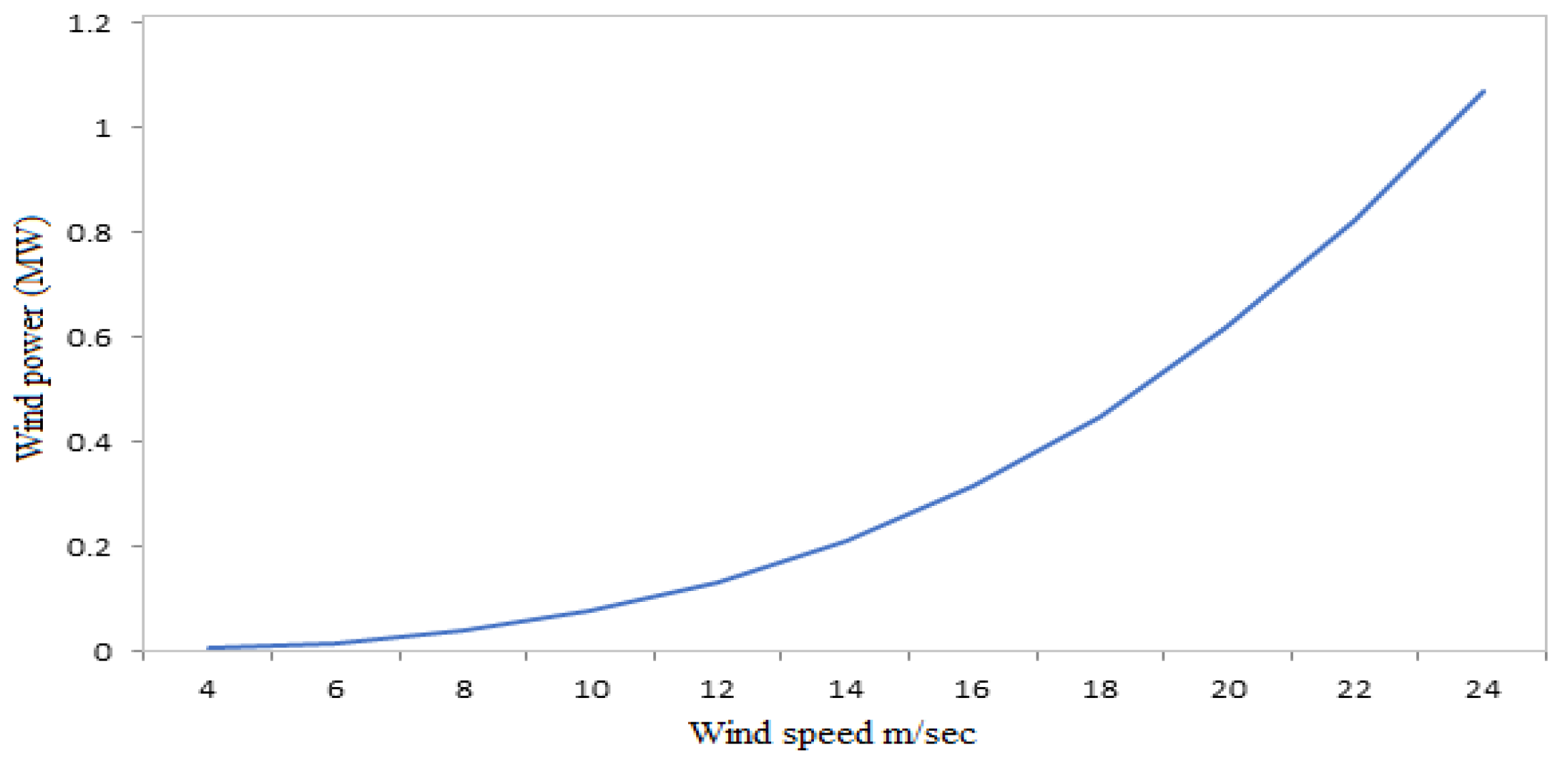
  • Power can be generated only between the cut-in speed (4 m/s) to cut-out speed (24 m/s).
A wind rose diagram depends on the wind direction where the wind turbine has to face the wind speed to extract maximum wind power. Therefore, the wind speed direction for every hour, day, week, month, and year are essential to analyze the wind characteristics. Winds directions are classified as 0 degrees to 360 degrees and are divided into either part (N, NE, E, SE, S, SW, W, and NW).
Additionally, statistics examination of the computed wind data in the Radhapuram wind pooling substation is carried out. Wind parameter functions are implemented to assess the accuracy of the statistic best wind speeds, wind power, and El Niño of the selected site. Furthermore, the distribution technique is employed for parameter approximation related to other wind parameters like temperature, pressure, etc. The open-source python platform with an in-house established program code is employed for approximating the parameters of wind investigation. It was specified previously that the best fit to estimate the finest wind power scheme was with a lesser proportion of RMSE rate closer to zero. As well, the greater level of R2 must be closer to 1, which condenses the error fitting for assessing the WPD. Moreover, the consequences are congregated for the finest wind power and speed with the nominated distribution. Far along, the yearly mean wind speed (MWS) and mean turbulence intensity are taken to sort the class of turbulence, and this helps select the wind turbine to develop a standalone wind farm. For this study, a total of 40 years (1980 to 2020) of wind parameter data has been taken. The statistical analysis is carried out using several functions such as mean, median, mode, range, variance, standard deviation, skewness, and Kurtosis.

5. Results and Discussions

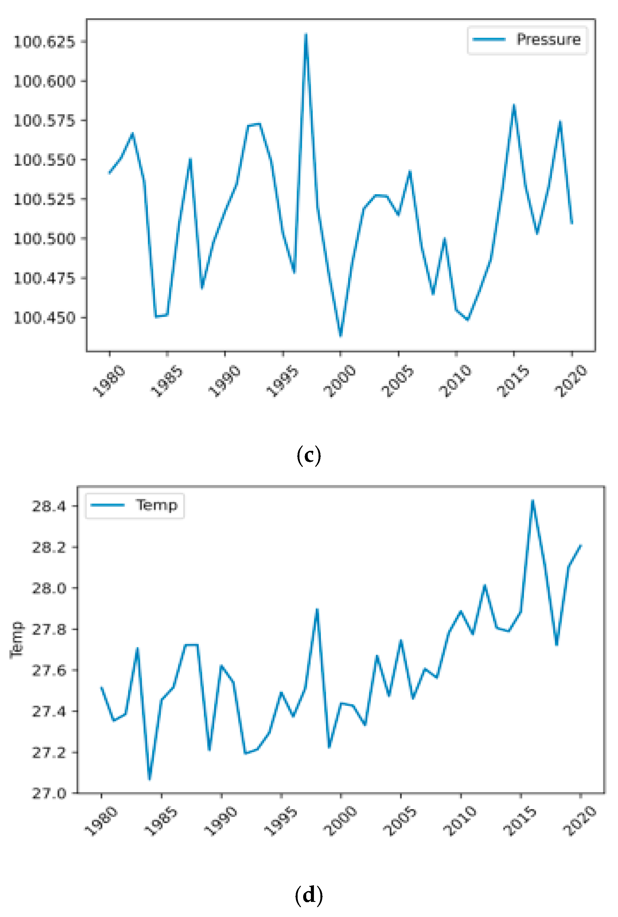
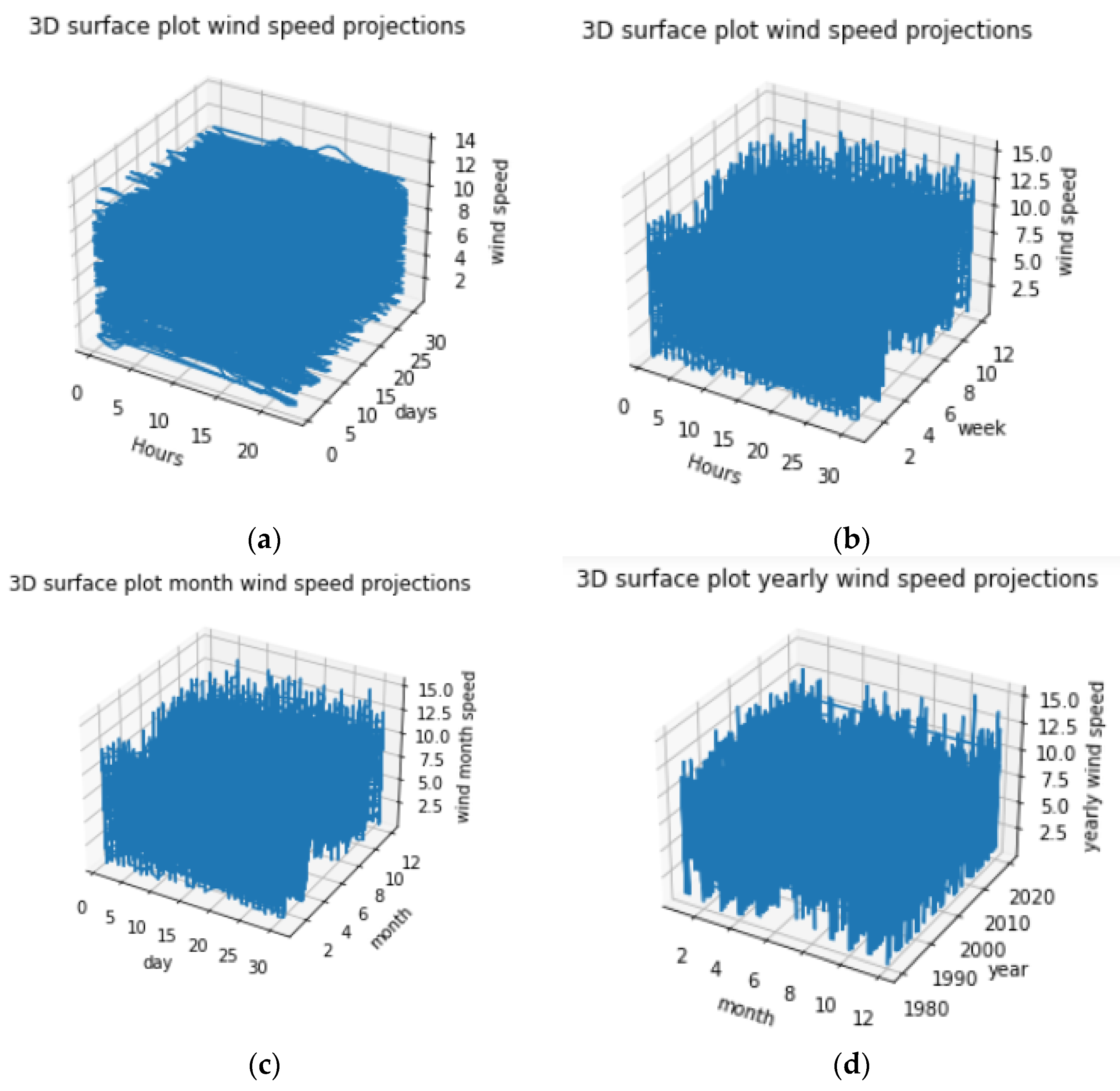
5.1. Wind Characteristics Investigation

In this study, the Radhapuram (Tamilnadu State, India) wind farms are considered as a case study. The maximum power extract from the direction is mainly from N, NE, S, SW, and W and other directions have less wind power (less wind speed). So, a wind speed’s direction displays an important role in extracting wind power season-wise by winter, summer, southwest monsoon, and northeast monsoon. The other parameters, such as pressure and temperature, also play an important role in wind characteristics.
The yearly mean wind speed, maximum wind speed, and standard deviation in the Radhapuram area for the period 1980 to 2020 are considered for this study. The highest minimum wind speed of 6.07 m/s was logged on 26 April 1981 and 28 October 1987, and a higher wind speed of about 15.49 m/s on 30 November 2017 and an MWS of 6.072 m/s for an average of 40 years and the wind speed at several elevations is measured. This was perceived for diverse ranges, notably 4 m/s wind speed to 24 m/s, and the power extract from the wind speed is in Table 5. Furthermore, the relationships between wind speed, wind power, and hub height are illustrated in Figure 5 and Figure 6.
The peak seasonal wind speed on the SWM is about 13.71 m/s, and the higher seasonal speed is detected as 15.52 m/s. Compared with monsoon periods (Table 6), northeast monsoon (NEM) realizes a stumpy mean speed of about 5.46 m/s. The monthly MWS is seen as higher, particularly in June, and its value is about 7.79 m/s, but the maximum speed in July is recorded as 15.49 m/s. Furthermore, the standard deviation for the month case is observed and found to be stable from January to March (2.2 m/s). Due to seasonal wind speeds in the monsoon period, May, July, and October were observed as 6.42 m/s, 7.79 m/s, and 7.25 m/s, respectively. Furthermore, the selected location, the Radhapuram wind location, comes under ‘B’ turbulence category as per IEC standard with 0.132 MTI at 15 m/s, i.e., 13.2%.
For the yearly wind measurements at 100 m hub height, turbulence intensity and wind speed are recorded for different altitudes; wind speed upturns in greater latitudes. Initially, the wind speed reaches 2 m/s at 10 m hub height, and it further increases to 4 m/s for 100 m of hub height. To extract higher power, it is essential to erect the wind turbines at possible higher altitudes since wind power generation is a cubic of speed. For 2015, observed wind speed is insignificant and inferior compared to 2014 and 2015 because of climatic variations. To ensure these inferences, the wind rose plots for different seasons are illustrated in Figure 7.
In the wind rose chart, the light color signifies a stumpy wind power generation during low wind speed, and the wind turbine’s cut-in speed would be 3 m/s. When the cut-in-speed increases beyond a certain level, power generation from a wind turbine rises, which is illustrated as a dark color and is densely spaced. It is vibrant from the wind rose figure; the power production of wind turbine, wind direction, and its speed are correlated. The wind turbine produces higher power when the wind blows from a direction between 0–90 and 180–225 degrees. From the wind rose figure, it is also perceived that power generation occurs when the speed exceeds the cut-out speed (22 m/s). Similarly, light wind speed and low power generation emerge from directions (90 to 180 and 270 to 360). The radius of the wind incidence denotes the wind direction parameter rose diagram.
Furthermore, the seasonal wind parameter distribution is observed for winter, summer, southwest monsoon (SWM), and northeast monsoon (NEM), and the graphical illustrations are depicted in Figure 8. In addition, other parameters, namely wind directions, wind speed, El Niño, temperature, pressure, and wind power, are observed, and their maximum and minimum values, standard deviation, and mean values are computed in Table 7. Eventually, the wind characteristics of the selected site against hour, day, month, and year are demonstrated in Figure 8 with reference to a 100 m hub height. Also, wind speed, El Niño, pressure, and temperature of the Radhapuram site are simulated for hourly, daily, monthly, and yearly. The graphical representations of the annual plots are given in Figure 9. It is observed that there is evidence of continual changes of parameters throughout the considered duration.

5.2. Statistical Analysis

A practical graphical approach is adopted to evaluate the kurtosis and wind speed skewness of the data set, i.e., histogram. The magnitude of variance is more prominent for a broader wind speed and smaller for a narrow kind. Standard deviation can be determined considering the root square variance using the variation between the individual speed data point and the mean value. It is possible for a more significant wind speed deviation within the date when it attains points farther from the mean value; however, a closer point to the mean value represents a lower deviation. The complete descriptions of the parameters for wind speed are illustrated in Table 8. The mean, standard deviation, maximum, and minimum wind speed parameters are 6.07 m/s, 2.12 m/s, 13.46 m/s, and 0.29 m/s, respectively. Similarly, wind power and El Niño effects are assessed.

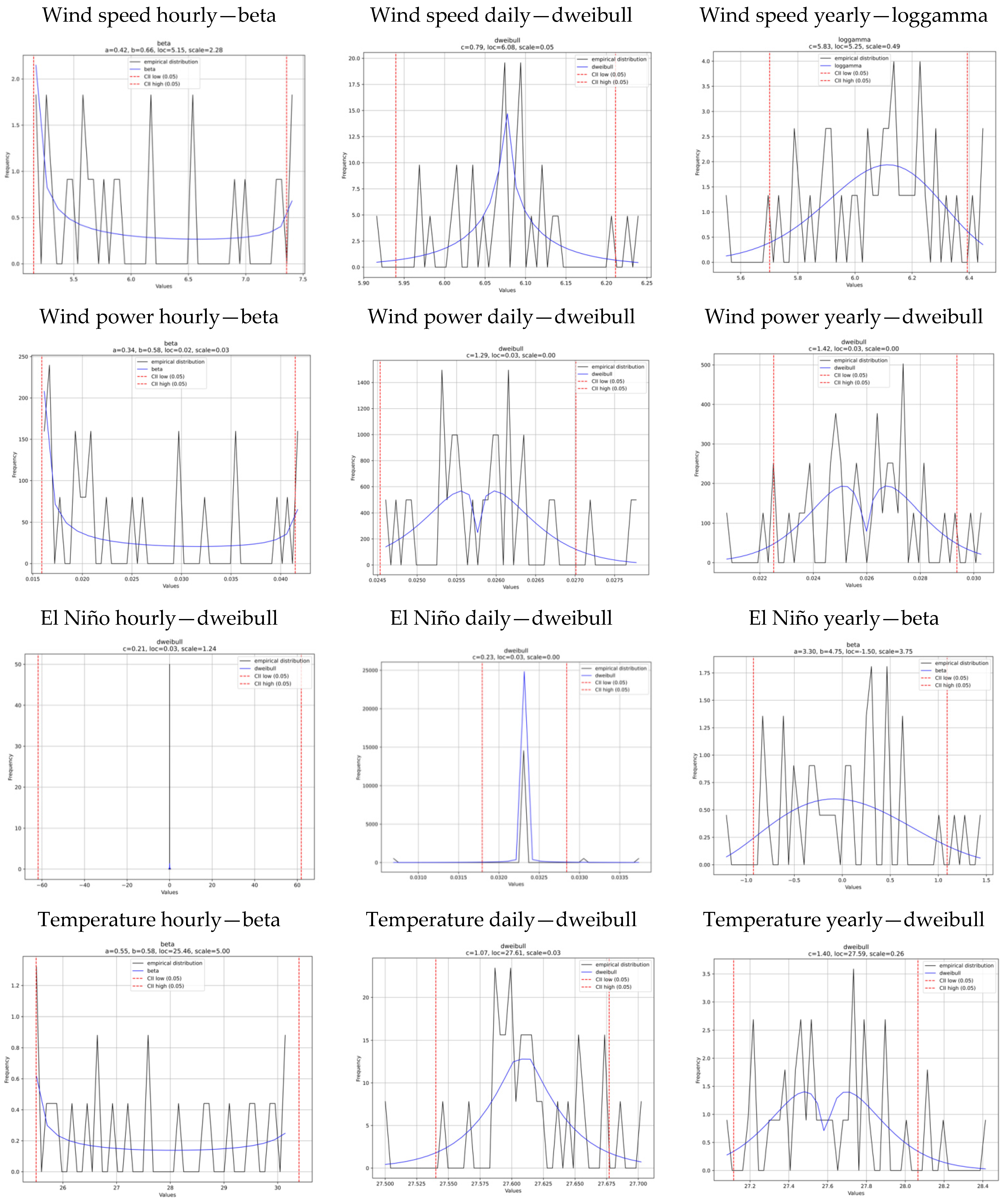
5.3. Wind Distribution Fitting

The wind distribution fitting for the Radhapuram polling station is assessed using different distribution functions for four different seasons, such as winter, summer, SWM and NEM, and the observed values are depicted in Table 9. From the observed results, it is perceived that the mean value of SWM offers better values compared with other seasons.
Furthermore, the estimated parameters of the Radhapuram station for Bimodal are assessed and shown in Table 10, and symbolic representation is demonstrated in Figure 10 (distribution pattern).

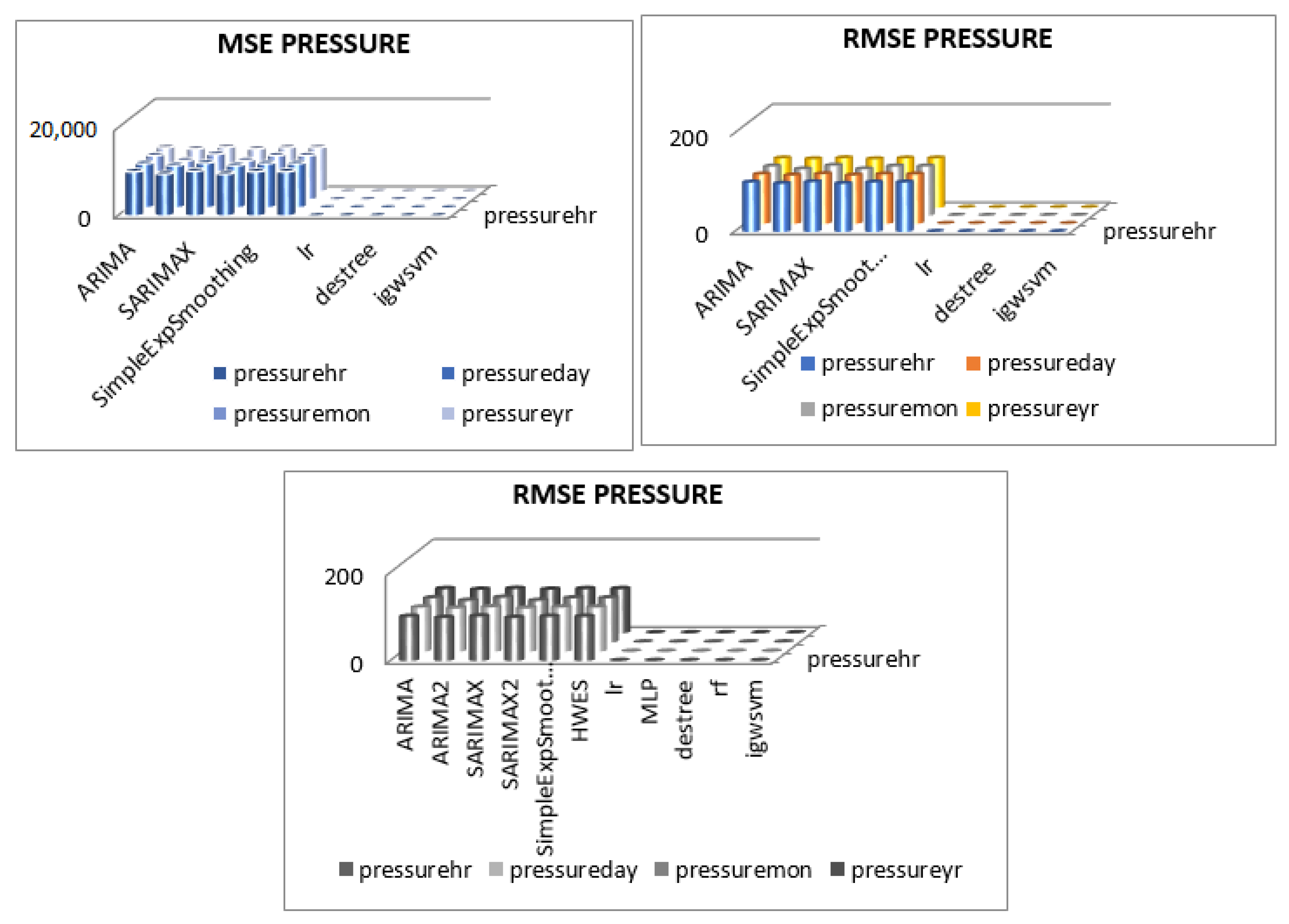
5.4. Wind Forecasting Analysis

Precise wind-haste predicting is vital for sustainable power development scheduling and the functioning of a power system. Figure 11 displays the deviation fashion of wind power for an hour, month, week, and year, assuming the probable substantial wind power near the spaces and those wind plants situated in the demand center [46], with the Radhapuram wind farms receiving higher attention in Tamilnadu. Similarly, wind speed for the same case is illustrated in Figure 12 using the 3D model.
The optimized parameters of the SVR model are considered to predict the wind speed data, notably by selecting random parameters C of 2 and g of 1. It symbolizes the SVR method with optimization based on four criteria including MAE, MSE, and RMSE. The hybrid IGWO-SVR approaches have agreeable performance in wind speed, and wind power forecasts since the predicting curves are close to the actual wind speed curve. The plotted figures show that the predicting curve of IGWO-SVR is closer to the actual zero error of wind speed data, particularly for the hourly and day-ahead prediction.
To ensure the accuracy of the proposed model, wind power, wind speed, El Niño, temperature, and pressure of the Radhapuram polling station are forecasted and illustrated in Figure 13, Figure 14, Figure 15, Figure 16 and Figure 17. The forecasting approaches effectively predict the non-stationary wind speed, and all predicting models show acceptable presentation. Taking the steps-forward forecast as an instance, the MAE errors of the common ARIMA, linear regression, decision tree, random forest, and IGWO-SVR are 1.2602, 1.2616, 1.2761, 1.2605, and 1.2386, respectively. All the evaluation metrics for all parameters show better ranges for different forecasting periods than other considered conventional methods. The enactment of the optimized SVR approaches are grander than the SVR model with C and g scales of 2 and 1, respectively. The IGWO-SVR model shows better outcomes among other considered optimization models.

6. Conclusions

This study proposes a novel hybrid technique, namely IGWO-SVR, to forecast wind parameter characteristics and distribution functions at different timescales, likely hourly, daily, monthly, seasonally, and annually. With this model, wind characteristic investigation is performed to study the relationships between wind speed, wind power, and hub height. Statistical analysis is carried out to evaluate the seasonal behavior of the location using notable parameters. Moreover, wind distribution fitting is demonstrated using beta, dweibull, exponential, gamma, genextreme, logamma, lognorm, parento, and uniform, and simulated for individual months and seasons such as winter, summer, NEM, and SWM. Finally, a wind forecasting event is simulated and the reliability of the observed results is verified using different evaluation metrics such as MAE, MSE, and RMSE. Additionally, the attained accuracy of the metrics are compared with other existing models such as ARIMA, ARIMA 2, SARIMAX, SARIMAX 2, simple exponential, linear regression, decision tree, and random forest. The proposed IGWO-SVR offers better results. Based on the results, the following conclusions are drawn:
  • The prevailing wind direction for Radhapuram was observed as S (15.8%) and SW (13.05%) from the southwest monsoon. The northeast monsoon fetches low wind and prevailing wind direction with a wind speed of about 11.07% (NE) and a north direction of 10.17%. The WPD density was measured at 100 m height at Radhapuram, the highest value of about 431.53 watts/m2.
  • The annual mean wind speed was better at about 7.51 m/s, and the wind rose diagram showed the maximum wind speed prediction in the southwest monsoon and northeast monsoon seasons.
  • Compared with various other time series forecasting analysis models, the proposed hybrid IGWO-SVR method offers the best minimum error values of MAE, MSE, and RMSE.
This research outcome greatly helps investment in potential wind farms by forecasting the wind parameters obtained through the proposed IGWO-SVR method.

Author Contributions

Conceptualization, S.S.H. and R.R.; methodology, S.S.H. and R.R.; software, S.S.H. and R.R.; validation, S.S.H., R.R. and K.R.; formal analysis, R.R. and K.R.; investigation, S.S.H., R.R. and G.S.; supervision, R.R. and G.S.; writing—original draft, S.S.H. and R.R.; writing—review and editing, S.S.H., R.R., K.R. and G.S. All authors have read and agreed to the published version of the manuscript.

Funding

This research received no external funding.

Institutional Review Board Statement

Not applicable.

Informed Consent Statement

Not applicable.

Data Availability Statement

Not applicable.

Conflicts of Interest

The authors declare no conflict of interest.

References

  1. Venkatesan, C.; Kannadasan, R.; Alsharif, M.H.; Kim, M.-K.; Nebhen, J. Assessment and Integration of Renewable Energy Resources Installations with Reactive Power Compensator in Indian Utility Power System Network. Electronics 2021, 10, 912. [Google Scholar] [CrossRef]
  2. Rajalakshmi, M.; Chandramohan, S.; Kannadasan, R.; Alsharif, M.H.; Kim, M.-K.; Nebhen, J. Design and Validation of BAT Algorithm Based Photovoltaic System Using Simplified High Gain Quasi Boost Inverter. Energies 2021, 14, 1086. [Google Scholar] [CrossRef]
  3. Balaguru, V.S.S.; Swaroopan, N.J.; Raju, K.; Alsharif, M.H.; Kim, M.-K. Techno-Economic Investigation of Wind Energy Potential in Selected Sites with Uncertainty Factors. Sustainability 2021, 13, 2182. [Google Scholar] [CrossRef]
  4. Shafiullah, G.M.; Oo, A.; Ali, S.; Wolfs, P. Potential challenges of integrating large-scale wind energy into the power grid—A review. Renew. Sustain. Energy Rev. 2013, 20, 306–321. [Google Scholar] [CrossRef]
  5. Shafiullah, G.M.; Oo, A.; Ali, S.; Jarvis, D.; Wolfs, P. Economic analysis of Hybrid Renewable Model for Subtropical Climate. Int. J. Therm. Environ. Eng. IJTEE 2010, 1, 57–65. [Google Scholar] [CrossRef] [Green Version]
  6. Cheand, J.; Wang, J. Short-term load forecasting using a kernel-based support vector regression combination model. Appl. Energy 2014, 132, 602–609. [Google Scholar]
  7. Elavarasan, R.M.; Selvamanohar, L.; Raju, K.; Vijayaraghavan, R.R.; Subburaj, R.; Nurunnabi, M.; Khan, I.A.; Afridhis, S.; Hariharan, A.; Pugazhendhi, R.; et al. A Holistic Review of the Present and Future Drivers of the Renewable Energy Mix in Maharashtra, State of India. Sustainability 2020, 12, 6596. [Google Scholar] [CrossRef]
  8. Anthony, M.; Prasad, V.; Kannadasan, R.; Mekhilef, S.; Alsharif, M.H.; Kim, M.-K.; Jahid, A.; Aly, A.A. Autonomous Fuzzy Controller Design for the Utilization of Hybrid PV-Wind Energy Resources in Demand Side Management Environment. Electronics 2021, 10, 1618. [Google Scholar] [CrossRef]
  9. Chen, Y.; Yang, Y.; Liu, C.; Li, C.; Li, L. A hybrid application algorithm based on the support vector machine and artificial intelligence: An example of electric load forecasting. Appl. Math. Model. 2015, 39, 2617–2632. [Google Scholar] [CrossRef]
  10. Kong, P.; Chen, L.; Jing, M.A. Short-Term power load forecasting based on the fuzzy information granulation and SVM. Electr. Power Inf. Commun. Technol. 2016, 11–14. [Google Scholar] [CrossRef]
  11. Xia, C.; Zhang, M.; Cao, J. A hybrid application of soft computing methods with wavelet SVM and neural network to electric power load forecasting. J. Electr. Syst. Inf. Technol. 2018, 5, 681–696. [Google Scholar] [CrossRef]
  12. Shafiullah, G.M.; Arif, M.T.; Oo, A.M.T. Mitigation strategies to minimize potential technical challenges of renewable energy integration. Sustain. Energy Technol. Assess. 2018, 25, 24–42. [Google Scholar] [CrossRef]
  13. Jamal, T.; Urmee, T.; Shafiullah, G.M. Planning of off-grid power supply systems in remote areas using multi-criteria decision analysis. Energy 2020, 201, 117580. [Google Scholar] [CrossRef]
  14. Raju, K.; Elavarasan, R.M.; Mihet-Popa, L. An Assessment of Onshore and Offshore Wind Energy Potential in India Using Moth Flame Optimization. Energies 2020, 13, 3063. [Google Scholar] [CrossRef]
  15. Yu, J.; Fu, Y.; Yu, Y.; Wu, S.; Wu, Y.; You, M.; Guo, S.; Li, M. Assessment of Offshore Wind Characteristics and Wind Energy Potential in Bohai Bay, China. Energies 2019, 12, 2879. [Google Scholar] [CrossRef] [Green Version]
  16. Rezaeiha, A.; Montazeri, H.; Blocken, B. A framework for preliminary large-scale urban wind energy potential assessment: Roof-mounted wind turbines. Energy Convers. Manag. 2020, 214, 112770. [Google Scholar] [CrossRef]
  17. Kumar, M.B.H.; Balasubramaniyan, S.; Padmanaban, S.; Holm-Nielsen, J.B. Wind Energy Potential Assessment by Weibull Parameter Estimation Using Multiverse Optimization Method: A Case Study of Tirumala Region in India. Energies 2019, 12, 2158. [Google Scholar] [CrossRef] [Green Version]
  18. Hulio, Z.H.; Jiang, W. Wind energy potential assessment for KPT with a comparison of different methods of determining Weibull parameters. Int. J. Energy Sect. Manag. 2020, 14, 59–84. [Google Scholar] [CrossRef]
  19. Mohammadi, K.; Alavi, O.; McGowan, J.G. Use of Birnbaum-Saunders distribution for estimating wind speed and wind power probability distributions: A review. Energy Convers. Manag. 2017, 143, 109–122. [Google Scholar] [CrossRef]
  20. De Andrade, C.F.; Dos Santos, L.F.; Macedo, M.V.S.; Rocha, P.A.C.; Gomes, F.F. Four heuristic optimization algorithms applied to wind energy: Determination of Weibull curve parameters for three Brazilian sites. Int. J. Energy Environ. Eng. 2018, 10, 1–12. [Google Scholar] [CrossRef] [Green Version]
  21. Idriss, A.I.; Ahmed, R.A.; Omar, A.I.; Said, R.K.; Akinci, T.C. Wind energy potential and micro-turbine performance analysis in Djibouti-city, Djibouti. Eng. Sci. Technol. Int. J. 2020, 23, 65–70. [Google Scholar] [CrossRef]
  22. Bataineh, K.M.; Dalalah, D. Assessment of wind energy potential for selected areas in Jordan. Renew. Energy 2013, 59, 75–81. [Google Scholar] [CrossRef]
  23. Abas, H.; Vahid, R.; Simin, R. Wind energy potential assessment in order to produce electrical energy for case study in Divandareh, Iran. In Proceedings of the International Conference on Renewable Energy Research and Applications, Milwaukee, WI, USA, 19–22 October 2014. [Google Scholar]
  24. Teimourian, A.; Bahrami, A.; Teimourian, H.; Vala, M.; Huseyniklioglu, A.O. Assessment of wind energy potential in the southeastern province of Iran. Energy Sources Part A Recover. Util. Environ. Eff. 2019, 42, 329–343. [Google Scholar] [CrossRef]
  25. Gul, M.; Tai, N.; Huang, W.; Nadeem, M.H.; Yu, M. Assessment of Wind Power Potential and Economic Analysis at Hyderabad in Pakistan: Powering to Local Communities Using Wind Power. Sustainability 2019, 11, 1391. [Google Scholar] [CrossRef] [Green Version]
  26. Nasrabadi, M.S.; Sharafi, Y.; Tayari, M. A parallel grey wolf optimizer combined with opposition-based learning. In Proceedings of the 2016 1st Conference on Swarm Intelligence and Evolutionary Computation (CSIEC), Bam, Iran, 9–11 March 2016. [Google Scholar]
  27. Shafiullah, G.M. Hybrid Renewable Energy Integration (HREI) System for Subtropical Climate in Central Queensland. Renew. Energy 2016, 96, 1034–1053. [Google Scholar] [CrossRef]
  28. Joshua, V.; Priyadharson, S.M.; Kannadasan, R. Exploration of Machine Learning Approaches for Paddy Yield Prediction in Eastern Part of Tamilnadu. Agronomy 2021, 11, 2068. [Google Scholar] [CrossRef]
  29. Wind Power Profile of Tamilnadu State. Indianwindpower.com Web Portal. Available online: http://indianwindpower.com/pdf/Wind-Power-Profile-of-Tamilnadu-State.pdf (accessed on 2 March 2020).
  30. Feng, J.L.; Hong, K.; Shyi, K.; Ying, H.; Tian, C. Study on Wind Characteristics Using Bimodal Mixture Weibull Distribution for Three Wind Sites in Taiwan. J. Appl. Sci. Eng. 2014, 17, 283–292. [Google Scholar]
  31. Seshaiah, V.; Indhumathy, D. Analysis of Wind Speed at Sulur -A Bimodal Weibull and Weibull Distribution. Int. J. Latest Eng. Manag. Res. 2017, 2, 29–37. [Google Scholar]
  32. Venkatesan, C.; Kannadasan, R.; Alsharif, M.H.; Kim, M.-K.; Nebhen, J. A Novel Multiobjective Hybrid Technique for Siting and Sizing of Distributed Generation and Capacitor Banks in Radial Distribution Systems. Sustainability 2021, 13, 3308. [Google Scholar] [CrossRef]
  33. Venkatesan, C.; Kannadasan, R.; Ravikumar, D.; Loganathan, V.; Alsharif, M.H.; Choi, D.; Hong, J.; Geem, Z.W. Re-Allocation of Distributed Generations Using Available Renewable Potential Based Multi-Criterion-Multi-Objective Hybrid Technique. Sustainability 2021, 13, 13709. [Google Scholar] [CrossRef]
  34. Mirjalili, S.; Mirjalili, S.M.; Lewis, A. Grey wolf optimizer. Adv. Eng. Softw. 2014, 69, 46–61. [Google Scholar] [CrossRef] [Green Version]
  35. Gaidhane, P.J.; Nigam, M.J. A hybrid grey wolf optimizer and artificial bee colony algorithm for enhancing the performance of complex systems. J. Comput. Sci. 2018, 27, 284–302. [Google Scholar] [CrossRef]
  36. Long, W.; Jiao, J.; Liang, X.; Cai, S.; Xu, M. A random opposition-based learning grey wolf optimizer. IEEE Access 2019, 7, 113810–113825. [Google Scholar] [CrossRef]
  37. Bigdeli, N.; Afshar, K.; Gazafroudi, A.S.; Ramandi, M.Y. A comparative study of optimal hybrid methods for wind power prediction in wind farm of Alberta, Canada. Renew. Sustain. Energy Rev. 2013, 27, 20–29. [Google Scholar] [CrossRef]
  38. Ren, G.; Wen, S.; Yan, Z.; Hu, R.; Zeng, Z. Power load forecasting based on support vector machine and particle swarm optimization. In Proceedings of the 2016 12th World Congress on Intelligent Control and Automation (WCICA), Guilin, China, 12–15 June 2016; pp. 2003–2008. [Google Scholar]
  39. Gao, L.; Zhao, S.; Gao, J. Application of artificial fish-swarm algorithm in SVM parameter optimization selection. Comput. Eng. Appl. 2013, 49, 86–90. [Google Scholar]
  40. Samadzadegan, F.; Hasani, H.; Schenk, T. Simultaneous feature selection and SVM parameter determination in classification of hyperspectral imagery using Ant Colony Optimization. Can. J. Remote Sens. 2012, 38, 139–156. [Google Scholar] [CrossRef]
  41. Ranaee, V.; Ebrahimzadeh, A.; Ghaderi, R. Application of the PSOSVM model for recognition of control chart patterns. ISA Trans. 2011, 49, 577. [Google Scholar] [CrossRef] [PubMed]
  42. Afroz, Z.; Shafiullah, G.M.; Urmee, T.; Higgins, G. Prediction of indoor temperature in an institutional building. Energy Procedia 2017, 142, 1860–1866. [Google Scholar] [CrossRef]
  43. Salcedo-Sanz, S.; Ortiz-García, E.G.; Perez-Bellido, A.M.; Portilla-Figueras, A.; Prieto, L. Short termwind speed prediction based on evolutionary support vector regression algorithms. Expert Syst. Appl. 2011, 38, 4052–4057. [Google Scholar] [CrossRef]
  44. Sanz, S.S.; Ortiz-Garci, E.G.; Pérez-Bellido, Á.M.; Portilla-Figueras, A.; Prieto, L.; Paredes, D.; Correoso, F. Performance comparison of multilayer perceptrons and support vectormachines in a short-termwind speed prediction problem. Neural Netw. World 2009, 19, 37–51. [Google Scholar]
  45. Wang, Y.; Wu, D.L.; Guo, C.X.; Wu, Q.H.; Qian, W.Z.; Yang, J. Short-term wind speed prediction using support vector regression. In Proceedings of the IEEE Power and Energy Society General Meeting, Minneapolis, MN, USA, 25–29 July 2010. [Google Scholar]
  46. Kisi, J.; Shiri, S.; Karimi, S.; Shamshirband, S.; Motamedi, D.; Petković, D.; Hashimd, R. A survey of water level fluctuation predicting in Urmia Lake using support vector machine with firefly algorithm. Appl. Math. Comput. 2015, 270, 731–743. [Google Scholar] [CrossRef]
Figure 1. Radhapuram wind pooling station location: (a) map view, (b) site view.
Sustainability 14 04235 g001
Figure 2. (a) Parameters of GWO (b) 2D and (c) 3D DLH and possible next locations.
Sustainability 14 04235 g002
Figure 3. Position updating of IGWO.
Sustainability 14 04235 g003
Figure 4. Flowchart of IGWO-SVR algorithms.
Sustainability 14 04235 g004
Figure 5. Relationship between wind speed and wind power.
Sustainability 14 04235 g005
Figure 6. Relationship between wind speed and hub height.
Sustainability 14 04235 g006
Figure 7. Wind rose plot of the Radhapuram station for various time durations.
Sustainability 14 04235 g007aSustainability 14 04235 g007bSustainability 14 04235 g007c
Figure 8. Seasonal wind parameter distribution: (a) winter, (b) summer, (c) SEM, and (d) NEM.
Sustainability 14 04235 g008aSustainability 14 04235 g008b
Figure 9. (a) Wind speed, (b) El Niño, (c) pressure, and (d) temperature of the Radhapuram site at 100 m hub height.
Sustainability 14 04235 g009aSustainability 14 04235 g009b
Figure 10. Wind distribution pattern for wind speed, power, El Niño, temperature, and power.
Sustainability 14 04235 g010aSustainability 14 04235 g010b
Figure 11. Variation trend of wind speed (a) days, (b) weeks, (c) months, and (d) years.
Sustainability 14 04235 g011
Figure 12. 3D variation trends of the wind speed in (a) days, (b) weeks, (c) months, and (d) years.
Sustainability 14 04235 g012
Figure 13. Wind speed comparison of various models for the different forecasting period (wshr—hourly wind speed, wsday—daily wind speed, wsmonth—monthly wind speed, and wsyear—yearly wind speed).
Sustainability 14 04235 g013
Figure 14. Wind power comparisons of various models for the different forecasting period (wphr—hourly wind power, wpday—daily wind power, wpmonth—monthly wind power, and wpyear—yearly wind power).
Sustainability 14 04235 g014
Figure 15. Wind El Niño comparisons of various models for the different forecasting period (elnino hr—hourly El Niño, elninoday—daily El Niño, elnino mon—monthly El Niño, and elninoyr—yearly El Niño).
Sustainability 14 04235 g015
Figure 16. Temperature comparisons of various models for the different forecasting period (Temp hr—hourly temperature, Tempday—daily temperature, Tempmon—monthly temperature, and Tempyr—yearly temperature).
Sustainability 14 04235 g016
Figure 17. Pressure comparisons of various models for the different forecasting period (pressurehr—hourly pressure, pressureday—daily pressure, pressuremon—monthly pressure, and pressureyr—yearly pressure).
Sustainability 14 04235 g017
Table 1. Existing literature reports.
Ref. NoAlgorithmsDescriptions
[14]Moth flame optimization (MFO)
-
Steady wind speed was recorded in the Gulf of Khambhat (a part of Indian potential sites), stretching from 7 to 10 m/s.
-
This site provided the least turbulence intensity with a maximum wind power density (WPD) of about 431 watts/m2.
[15]Nakagami and Rician distributions (NCD)
-
The proposed method identified the key wind direction likely east, which recorded the wind speed stretching from 4 to 8 m/s.
-
The author concluded that Nakagami distribution displayed improved wind potential assessment.
[16]Distinctive wind-groups (DWG)
-
The author suggested a design to deal with a large scale and preliminary assessment at urban locations or small scales for roof-mounted turbine models.
-
Additionally, turbine characteristics and their numbers, annual energy production, metropolitan building data, and annual mean wind speed.
[17]Multiverse optimization
method (MO)
-
The authors reported the wind speed observed at the selected site was between 2 m/s and 10 m/s (direction 260–280°), and 0–4 m/s (sector 170–180°).
[18]Weibull parameters
-
This work assessed the wind shear coefficient and estimated it to be the least value of 0.18.
-
Additionally, mean wind speed and power density, standard deviation, and total energy output were figured for 30 and 10 m heights.
[19]Birnbaum–Saunders (BS) distribution
-
Presented the precision, generalization fitness, and efficiency of the BS distribution for demonstrating wind power and speed distribution.
[20]Harmony search (HS), cuckoo search optimization (CSO), particle swarm optimization (PSO), and ant colony optimization (ACO).
-
The author stated that the ACO method showed efficient performance for evaluating the functions of the Weibull distribution, notably for Triunfo and São Martinho da Serra.
-
In addition, CSO displayed better results for the Petrolina model.
[21]Weibull parameters
-
Recommended the likelihood to tool and progress the metropolitan wind energy sector for domestic applications.
-
Wind characteristics such as wind rose and power density were also investigated.
[22]Rayleigh
distribution
-
Addition to wind resource assessment, AEP, cost of energy, and capacity factors, were computed.
-
Total potential was estimated using several wind turbines ranging between 165 MW and 3 MW.
[23]Weibull probability density distribution
-
The authors considered four different turbine models and assessed for various constraints.
-
Additionally, this work reported the output energy of the turbine system, average power, capacity factor, and availability factor.
[24]Weibull distribution function
-
The author investigated the wind characteristics for monthly, seasonal, and annual wind speed variations.
-
Turbines were selected based on the site characteristic and computed different turbine parameters.
-
Additionally, the levelized energy cost was adapted to evaluate the monetary viability of electricity production.
[25]Weibull and
Rayleigh distribution functions
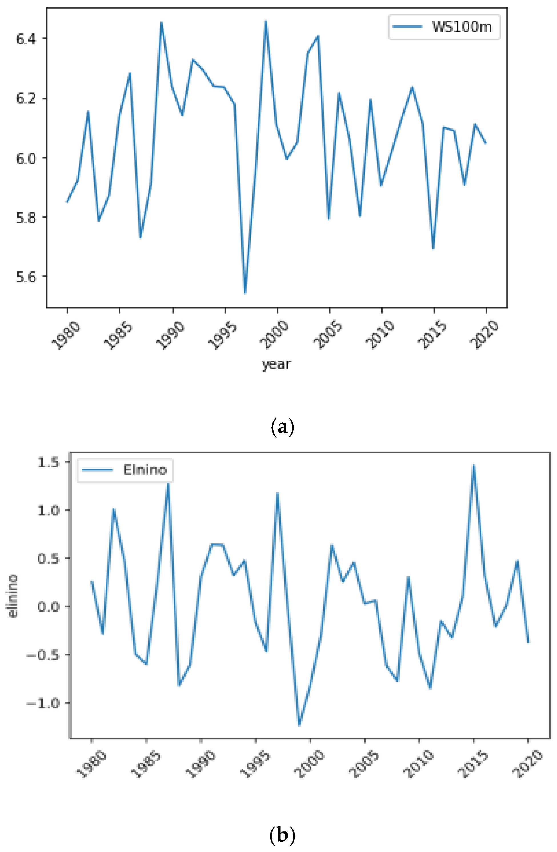
-
This work reported the mean speed of wind in the selected site was about 6 m/s for the whole year using the proposed methodology.
-
In addition, energy density and average wind power were assessed.
-
Turbines were modelled, and the output of the turbine, capacity factor, and cost of energy was estimated.
Table 2. Real-time data patterns range.
Input VariablesUnitsRange of Input Variables
Wind Speedm/s1–19
Wind DirectionDegree0.1–360
Air Pressurembar99–101
TemperatureDegree. Celsius17–45
El NiñoPercentage0.5–2
Wind PowerWm28–16
Table 3. Sensor’s measurement data from the Radhapuram wind pooling station.
Site NameLandmass
Meas. Sensor
Latitude and LongitudeDataset PeriodIntervalRecovery Rate
Radhapuram,
Tamilnadu
Satellite
ERA Data
N 8°16.140620′.
77°41′11.5368″
1980 to 2020
(41 years)
60 min100%
Table 4. Monsoon-based wind behavior.
SeasonMonthsDuration
WinterJanuary and FebruaryTwo months
SummerMarch to JuneFour months
SWMJuly to SeptemberThree months
NEMOctober to DecemberThree months
Table 5. Wind power of the Radhapuram station for various wind speeds.
S. NoWind Speed (m/s)Wind Power (MW)
140.004946
260.016693
380.039568
4100.07728
5120.1335
6140.2121
7160.31655
8180.4507
9200.61826
10220.8229
11241.0684
Table 6. Radhapuram wind directions—annual occurrence.
Direction SectorDirection NameMean
(m/s)
Max
(m/s)
Std. Dev.
(m/s)
Wind Occurrence
(%)
67.5° −90° −112.5°N3.1413.461.251.73
22.5° −45° −67.5°NE4.7620.631.826.51
337.5° −0° −22.5°E4.6213.382.242.84
292.5° −315° −337.5°SE4.2011.821.983.51
247.5° −270° −292.5°S3.4811.771.852.37
202.5° −225° −247.5°SW2.9710.111.531.86
157.5° −180° −202.5°W10.2622.863.3038.66
112.5° −135° −157.5°NW3.1113.481.351.88
Table 7. Wind parameters in the Radhapuram station.
Annual Parameter
(@100 m)
Wind SpeedWind DirectionEl NiñoTempPressureWind Power
Mean value6.072125178.533380.03235227.615456100.51492.586624 × 10−2
Standard deviation 2.475411104.28300.8548452.2027840.2502022.566458 × 10−2
Max. value 15.490000359.85002.60000036.100000101.4002.872362 × 10−1
Min value0.0700000.150000−0.80000020.20000099.50002.650813 × 10−8
25% of occurrence4.29000050.850000−0.50000026.000000100.3506.101784 × 10−3
50% of occurrence6.13500042.2000000.00000027.400000100.5001.784550 × 10−2
75% of occurrence7.900000259.550000.50000029.150000100.7003.810362 × 10−2
Table 8. Statistical Performance of the wind speed.
Wind SpeedCountMeanStdMaxMinVarSkewKurt
NEM90,5285.462.6015.490.076.760.200.71
SWM90,5286.881.9713.710.203.87−0.070.18
Summer120,0485.642.5314.000.076.380.180.63
Winter58,3206.652.4114.030.175.81−0.340.42
January30,5047.362.1814.030.214.75−0.590.23
February27,8165.872.4112.670.175.82−0.040.56
March30,5044.302.0011.780.134.020.310.39
April29,5204.061.8612.130.073.470.570.29
May30,5046.422.2813.710.305.18−0.020.44
June29,5207.791.8414.001.003.370.110.38
July30,5047.251.8813.620.573.54−0.030.25
August30,5047.011.8913.710.533.59−0.030.17
September29,5206.372.0213.510.204.07−0.040.23
October30,5044.662.1912.840.074.790.430.21
November29,5204.752.3315.490.105.440.330.49
December30,5046.962.5813.990.146.66−0.430.38
Annual 6.072.1213.460.29
Table 9. Seasonal wind distribution.
DistributionWinterSummerSWMNEM
beta0.00420.00130.01130.0037
dweibull0.01990.01400.01800.0205
expon0.25710.18310.37940.1445
gamma0.01590.00540.00960.0105
genextreme0.01130.00430.01160.0091
loggamma0.00350.00640.00970.0109
lognorm0.01310.00550.01030.0107
norm0.01240.00660.37030.0113
pareto0.26450.46930.01030.1421
t0.01240.00660.25920.0113
uniform0.16250.12910.12910.1291
Mean value0.00350.00130.00960.0037
Table 10. Radhapuram Bimodal Estimated Parameters.
distrbetadweibullexpongammagenextremeloggammalognormnormparetotuniform
Januaryscore0.00310.010.350.020.020.000.020.022.99 × 10−10.010.23
loc−703.87.500.21−26.336.594.94−416.67.36−2.50 × 1087.420.21
scale718.761.827.150.152.293.20423.962.182.50 × 1082.0513.82
Februaryscore0.010.010.240.010.010.010.010.012.28 × 10−10.010.13
loc−0.525.860.17−125.35.03−234.6−72.155.87−4.10 × 1085.870.17
scale13.4232.15.70.04452.442.07277.9882.44.10 × 1082.412.5
Marchscore0.000.040.260.010.010.010.010.012.84 × 10−10.010.22
loc0.004.200.13−3.133.50−484.1−8.234.30−1.49 × 1094.300.13
scale11.9791.84.20.55311.969.21812.36621.49 × 109211.7
Aprilscore0.000.010.320.000.000.010.000.016.77× 10−10.010.30
loc−0.303.960.07−1.463.27−599.7−4.244.06−1.534.020.07
scale18.4091.640.63751.680.518.09451.91.601.812.1
Mayscore0.000.010.270.010.000.010.010.012.78 × 10−10.010.18
loc−1.306.420.30−287.75.61−394.2−159.16.42−2.80 × 1086.420.30
scale15.35826.10.01762.360.96165.62.32.80 × 1082.313.4
Junescore0.010.020.430.010.010.020.010.026.96 × 10−10.020.29
loc−0.087.821.00−19.717.11−326.6−32.617.79−9.49 × 10−17.791.00
scale17.2611.76.80.12251.850.52340.361.81.941.813
Julyscore0.010.020.410.010.010.010.010.017.05 × 10−10.010.28
loc−2.617.330.57−125.26.57−277.0−84.467.25−1.027.250.57
scale18.2641.76.70.02681.944.82791.6961.91.591.913.1
Augustscore0.010.020.410.010.010.010.010.013.96 × 10−10.010.28
loc−4.267.060.53−117.46.31−279.7−134.47.01−1.26 × 1087.010.53
scale20.8331.76.50.02881.945.195141.361.91.26 × 1081.913.2
Septemberscore0.010.020.360.010.010.010.010.014.10 × 10−10.010.25
loc−3.266.430.20−100.95.62−245.9−195.36.37−4.86 × 1086.370.20
scale17.9681.76.20.038241.671201.6724.86 × 108213.3
Octoberscore0.000.020.230.000.000.010.000.012.39 × 10−10.010.20
loc−0.044.590.07−2.093.76−645.7−6.034.66−1.84 × 1084.660.07
scale14.3631.94.60.7278288.14510.4682.21.84 × 1082.212.8
Novemberscore0.010.020.160.010.010.020.010.021.56 × 10−10.020.17
loc0.004.670.10−1.853.79−636.6−6.984.75−1.87 × 1044.750.10
scale15.8292.14.70.86622.188.50111.4972.31.87 × 1042.315.4
Decemberscore0.010.020.250.030.020.010.020.022.30 × 10−10.020.15
loc−11.987.070.14−37.496.103.30−165.36.96−5.95 × 1086.960.14
scale26.3462.26.80.15852.74.0843172.292.65.95 × 1082.613.9
Winterscore0.000.020.260.020.010.000.010.012.64 × 10−10.010.16
loc−7.546.720.17−38.685.80−1.01−198.16.65−4.21 × 1066.650.17
scale21.6472.16.50.13252.55.1212204.792.44.21× 1062.413.9
Summerscore0.000.010.180.010.000.010.010.014.69 × 10−10.010.13
loc−0.075.640.07−8.214.69−581.9−18.425.64−1.50 × 1015.640.07
scale14.1012.35.60.4662.484.06923.9292.51.572.513.9
SWMscore0.010.020.380.010.010.010.010.013.70 × 10−10.010.26
loc−4.346.970.20−63.346.16−117.2−126.56.88−1.64 × 1086.880.20
scale20.011.76.70.0553224.563133.3321.64 × 108213.5
NEMscore0.000.020.140.010.010.010.010.011.42 × 10−10.010.13
loc−0.055.430.07−5.144.46646.23−14.345.461.85 × 1085.460.07
scale15.5622.45.40.65322.591.67919.6372.61.85 × 1082.615.4
Publisher’s Note: MDPI stays neutral with regard to jurisdictional claims in published maps and institutional affiliations.

