Article

Land-Use Impact on Water Quality of the Opak Sub-Watershed, Yogyakarta, Indonesia

by
Widodo Brontowiyono
1,2,
Adelia Anju Asmara
1,2,*,
Raudatun Jana
3,
Andik Yulianto
1,4 and
Suphia Rahmawati
1,4
1
Environmental Engineering Department, Universitas Islam Indonesia, Yogyakarta 55584, Indonesia
2
Center for Environmental Studies, Universitas Islam Indonesia, Yogyakarta 55584, Indonesia
3
Water Quality Laboratory, Universitas Islam Indonesia, Yogyakarta 55584, Indonesia
4
Risk Assessment Analysis Laboratory, Universitas Islam Indonesia, Yogyakarta 55584, Indonesia
*
Author to whom correspondence should be addressed.
Sustainability 2022, 14(7), 4346; https://doi.org/10.3390/su14074346
Submission received: 22 March 2022 / Revised: 31 March 2022 / Accepted: 1 April 2022 / Published: 6 April 2022

Abstract

:
The integrated monitoring system of water quality is eminently reliant on water quality trend data. This study aims to obtain water quality patterns related to land-use change over a periodic observation in the Opak sub-watershed, Indonesia, both from a seasonal and spatial point of view. Landsat image data from 2013 to 2020 and water quality data comprising 25 parameters were compiled and analyzed. This study observed that land use remarkably correlated to water quality, especially the building area representing the dense population and various anthropogenic activities, to pollute the water sources. Three types of pollutant sources were identified using principal component analysis (PCA), including domestic, industrial, and agricultural activities, which all influenced the variance in river water quality. The use of spatiotemporal-based and multivariate analysis was to interpret water quality trend data, which can help the stakeholders to monitor pollution and take control in the Opak sub-watershed. The results investigated 17 out of 25 water quality parameters, which showed an increasing trend from upstream to downstream during the observation time. The concentration of biological oxygen demand over five days (BOD5), chemical oxygen demand (COD), nitrite, sulfide, phenol, phosphate, oil and grease, lead, Escherichia coli (E. coli), and total coli, surpassed the water quality standard through spatial analysis.

1. Introduction

Rapid and vast land-use change generated environmental carrying capacity deterioration, thereby significantly decreasing water quality along with the watershed. According to some studies, green space and agricultural areas have changed extensively to become settlement and industrial areas in many big cities of Indonesia. For the last three decades in the primary watershed, which covered Jakarta, Bogor, Depok, Tangerang, and Bekasi (Jabodetabek), the building area grew more than 12 times and up to 30% of natural vegetation was lost [1]. Agricultural land in Kartamantul (Sleman, Yogyakarta and Bantul), Yogyakarta was converted into settlement area for 1.19%/year from 1994–2000 [2]. According to Statistics of D.I. Yogyakarta, from 2012 to 2014, 1149 Ha of agricultural land was converted to serve non-agricultural purposes in 3 regions of the Winongo River [3]. The upstream of the Brantas sub-watershed reported a drastic increase in the resident area from 2520.74 Ha to 4830.62 Ha in 7 years (2006–2013) [4]. As the change of land cover and land use related to quality and quantity of river water occurred, the Ministry of Environment and Forestry of Indonesia identified that more than 68% of water quality in all regions of Indonesia have been heavily polluted [5]. On the other hand, the Brantas Watershed has 421 fountains, which fell to 57 fountains in less than 5 years [6] and about 119 wellsprings in Kulonprogo. Yogyakarta has been identified as being critical and in an endangered status [7], and there are around 160 natural water sources in Bandung City, only 67 of which produce water [8]. Declining water quality encourages other serious problems associated with decreased water quality and public health risks.
Land cover and land use are critical components of water quality. Both point and non-point pollution sources from land use are pivotal issues to monitor watershed management and planning. Different contaminant sources run into nearby water bodies. For instance, ground and surface water aggravate water quality itself. Much research has been conducted to investigate the correlation between the effect of land use and water quality. Camara et al. found that 87% of urban land use was a significant source of water pollution [9].
In comparison, 82% identified agricultural land use, 77% forest land use and 44% other land uses. The correlation revealed that the related activity of agriculture and forest had a more significant impact on water quality due to their physical and chemical water quality indicators. At the same time, urban development activities are more affected due to changes in hydrological processes, such as runoff and erosion. Using satellite images from 2007 until 2017, Tahiru et al. found the impact of land use and land cover changes on water quality parameters, such as turbidity, ammonia, and total coliform counts [8]. Remote sensing and statistical analysis were employed to divide three ‘effluents’ of built-up areas, agriculture areas, and open space [10]. These groups significantly correlated to declining water quality, including Total Suspended Solids (TSS), Biochemical Oxygen Demand (BOD5), Chemical Oxygen Demand (COD), E. coli, and several metals. Another interesting finding was that of E. coli and sediment parameters in changing land use land cover using water quality index and modelling water discharge [11]. Over eight years, E. coli data was collected, and Landsat data between 2001 and 2018 was used and showed a negative correlation between E. coli loading and expanded land use land cover. In addition, the higher the water discharge, the more sediment loading is possible in the sub-basin.
Several approaches are utilized to investigate other relations between land use and various water contaminants, such as the pairing of spatial and multivariate statistical analysis. By understanding and observing numerous water quality parameters simultaneously and their related factors, principal component analysis (PCA) is applicable to support an interpretation of the results. Tripathi and Singal [12] applied PCA to represent 9 out of 28 water quality parameters that possessed significant results and less bias to determine Water Quality Index (WQI) in the Ganga River. Furthermore, Lee et al. [13] examined the correlation with a significant level (p < 0.05) and PCA on water quality parameters regarding land use covered. Each source positively associates with specific parameters; examples for the residential area are BOD5, COD, NH3, and PO4 while for agricultural land, examples are TSS, NO3, and PO4; as well as BOD5, COD, NH3, and NO3 for livestock. The integrated method by PCA/FA (principal component analysis/factor analysis), analysis of variance (ANOVA), and cluster analysis (CA) were employed to identify source pollution due to land-use changes in northern Iran [14]. Another particular result shows that most inorganic ions and land-use characteristics are examined for small river basins in central Japan [15]. The urban development and residential area showed a significant positive correlation to farmland-exposed, noticeable ions of pollutants.
Previous research has analyzed the relationship between land use and water quality measures in Indonesia. A study using the pollution index method in Semarang City indicated that the water pollution index was above government regulation standard [16]. Another study conducted by Nugraha [17] simulated the influence of land use on water quality via the QUAL2E model and pollution index in Central Java. Unfortunately, detailed spatial land-use data did not support that research. Moreover, research conducted by Indriyani et al. [18] exposed where BOD5 and COD loading from the residential area resulted in the worst water quality on the Ciracab River. Inversely, the forest area had opposite conditions. However, the land-use data were supported by GIS-based analysis data, only after being investigated for a few water parameters and lack of statistical analysis. In Yogyakarta, some investigations were done by combining spatial and multivariate analysis. Suharyo [19] and Hamid [20] studied the water quality of the Opak watershed. They found a positive correlation between chemical and microbial parameters and land use, although the multivariate analysis was not significant (r ≤ 0.5) due to limited temporal data. Munawar [21] and Pratama [22] did comprehensive and multi-analysis research on the Code River. The initial study explained not only the spatial data and water quality analysis but also economic analysis. Then, the later study coupled LULC (land use land change) and multivariate analysis.
Although many researchers have analyzed the relationship between land use and water quality, only a few of them utilized principal component analysis (PCA) in Indonesia. In addition, PCA analysis is an appropriate data representation technique to imagine and recognize the kind of pollutants in the Opak sub-watershed [23,24]. In the current study, a spatiotemporal analysis is applied on the water quality of the Opak sub-watershed focused on the Winongo River and its land use for the period of 2013–2020. PCA further analyzed the critical and selected data out of 25 water quality parameters at 8 sampling points to identify the possible pollution sources. Subsequently, the seven-year water quality trend data were analyzed by multivariate statistical correlation with land use.

2. Materials and Methods

2.1. Study Area

Opak watershed, located in Yogyakarta Province, Indonesia, has a length of 65 km and a catchment area of ±1398.18 km2. The watershed consists of the Tambakbayan, Code, Winongo, Gajahwong, and Oyo sub-watersheds. One of the biggest sub-watersheds that crosses three regions in Yogyakarta is the Winongo sub-watershed [25]. The Winongo River has a total coverage area of 47.83 km2. It has a length of 23.49 km, flowing from the upstream located on Sleman Regency and through the middle stream on Yogyakarta City, finishing downstream in Bantul Regency. The width of the surface rivers is averaged to about 10.2 m, while the width of the bottom is ranged around 8.5 m [26]. The Winongo River is a pivotal river for three regions of Yogyakarta, i.e., Sleman Regency, Yogyakarta City, and Bantul Regency, used for water drinking resources, irrigation, household cleaning, fish-farming, dams, sand quarries, and as a tourist destination.
The catchment area of the Winongo River of the Opak sub-watershed tends to decline, starting from 112 km2 (2002) [27], then decreasing to 88.12 km2 (2012) [28], and finally 47.83 km2 (2021). The average annual rainfall is 1466.55 mm/year and shows a drought index from 24.56% to 36.87% (mid to heavy drought), with a basin coefficient of 0.875 [29]. Statistics of D.I. Yogyakarta reported the average annual temperature to be about 26 °C; the maximum temperature in August is 34.8 °C and the minimum temperature in July is 18.40 °C. Furthermore, annual relative humidity is measured at ±86% [30]. Besides, urbanization and rapid population growth without proper control and management triggered many citizens to build their residence along the riverbank. In addition to coming from inside Yogyakarta, such as Wonosari and Kulon Progo, nonnative people came to Yogyakarta from Wonigiri, Solo, and Madura. This resulted in many issues that other cities in Indonesia also faced, such as heavily polluted rivers, high sedimentation, fast erosion level, and flooding [31,32,33]. Furthermore, the middle stream flows through the tight urban population and home industries caused various water contaminants to enter the sub-watershed [34,35,36]. Also, numerous fishery activities generate algae blooming phenomenoa in several river flow components [37,38].
In this study, the water quality of the sub-watershed was monitored in eight sampling points (S1–S8), spreading into three segments. Those segments were divided based on boundary administration and slope regions. The first segment upstream (UP1), whose 100–150 m of river slope was in the Sleman region, was then observed by the S1 station. Secondly, the middle stream (MD2) that sloped ranged from 50 to 100 m, which crossed the Yogyakarta City monitored by the S2 to S4 stations. The water quality of the sub-watersheds downstream (DW3) was sampled from the S5 to S8 stations laid on the Bantul region with a slope of fewer than 50 m. Table 1 shows the geocoordinates of sampling points. Furthermore, all the sampling locations and those segments were visualized in Figure 1.

2.2. Water Quality and Geographic Information

The water quality data of the sub-watershed was taken from the Environmental Agency of Yogyakarta Province from 2013 to 2020. The data was collected three times a year from the eight sampling stations explained before (S1–S8). Every monitoring data point consists of 25 parameters, which were physical parameters: temperature, pH, Total Dissolved Solids (TDS), Total Suspended Solids (TSS), and color; chemical parameters: Dissolved Oxygen (DO), Biochemical Oxygen Demand (BOD5), Chemical Oxygen Demand (COD), Chlorine (Cl2), nitrate (NO2), nitrite (NO3), ammonium (NH4), detergent, phenol, phosphate (PO4), oil and fat, iron (Fe), manganese (Mn), cadmium (Cd), lead (Pb), zinc (Zn), and copper (Cu); and biological parameters: Total coliform and E. coli.
For spatial processing data, two types of satellite images were used. First, land use classification data was extracted from Landsat data collected by the United States Geological Survey (USGS) from 2013 to 2020. Second, to determine the sub-watershed boundary, the satellite data was delineated and extracted by a mask manually using ArcGIS 10.8. Exact steps were defined for deciding river segments (upstream, middle stream, and downstream). The shapefile images were gathered from the Environmental Agency of Yogyakarta Province.

2.3. Land-Use Classification

ArcGIS 10.8 extracted and processed each satellite image of USGS from 2013 to 2020 and broken into layers. The land-use classification was based on the most similar images of training sample drawing tools, conducted by interactive supervised classification. After the final conversion, land uses were categorized and divided into the National Standard Indonesia (SNI 7645-1:2014) three main cover types, namely building (BU), agriculture (AG), and VA (Vegetation). Those categories were considered according to the dominant coverage area in three representative regions.

2.4. Statistical Analysis

Pearson correlation analysis was used to assess the close link between the data variables of water quality parameter in each sub-watershed and the quantity of land use utilized. To determine correlation coefficients, a correlation matrix was created by calculating the coefficients of different pairings of parameters, and the correlation was then checked for significance using the p valve. The significance was assessed at the 0.05 level (2-tailed analysis). If p < 0.05, the differences were substantial, and if p > 0.05, they were not. The Pearson correlation coefficient was appropriate for normally distributed data, whereas Spearman-rho (ρ) and Kendall-tau (σ) were not regularly distributed [39,40,41]. Besides the Pearson correlation, this study also applied principal component analysis (PCA) so that multivariate normal data could be obtained. The first stage in the PCA approach was to determine factor analysis and identify the original variables among sub-watershed water qualities. PCA analysis has initial eigenvalues greater than 1 supported by the rotation matrix method, containing the number of factors to be selected from the variable [42,43,44]. By following and interpreting, the rotation outcome factor was going to reveal factors and variables regarding the water quality in the Opak sub-watershed. Moreover, to validate, the PCA analysis was assessed by preliminary tests, such as the Kaiser–Meyer–Oklin (KMO) Test, Bartlett Test, anti-image, and scree plot. The KMO test was considered appropriate to use after reaching a value of one. The Bartlett and anti-image significant tests might be less than 0.5 [45,46]. Finally, the scree plot was evaluated to identify the number of elements or categories retrieved in a matrix [47].

3. Results and Discussion

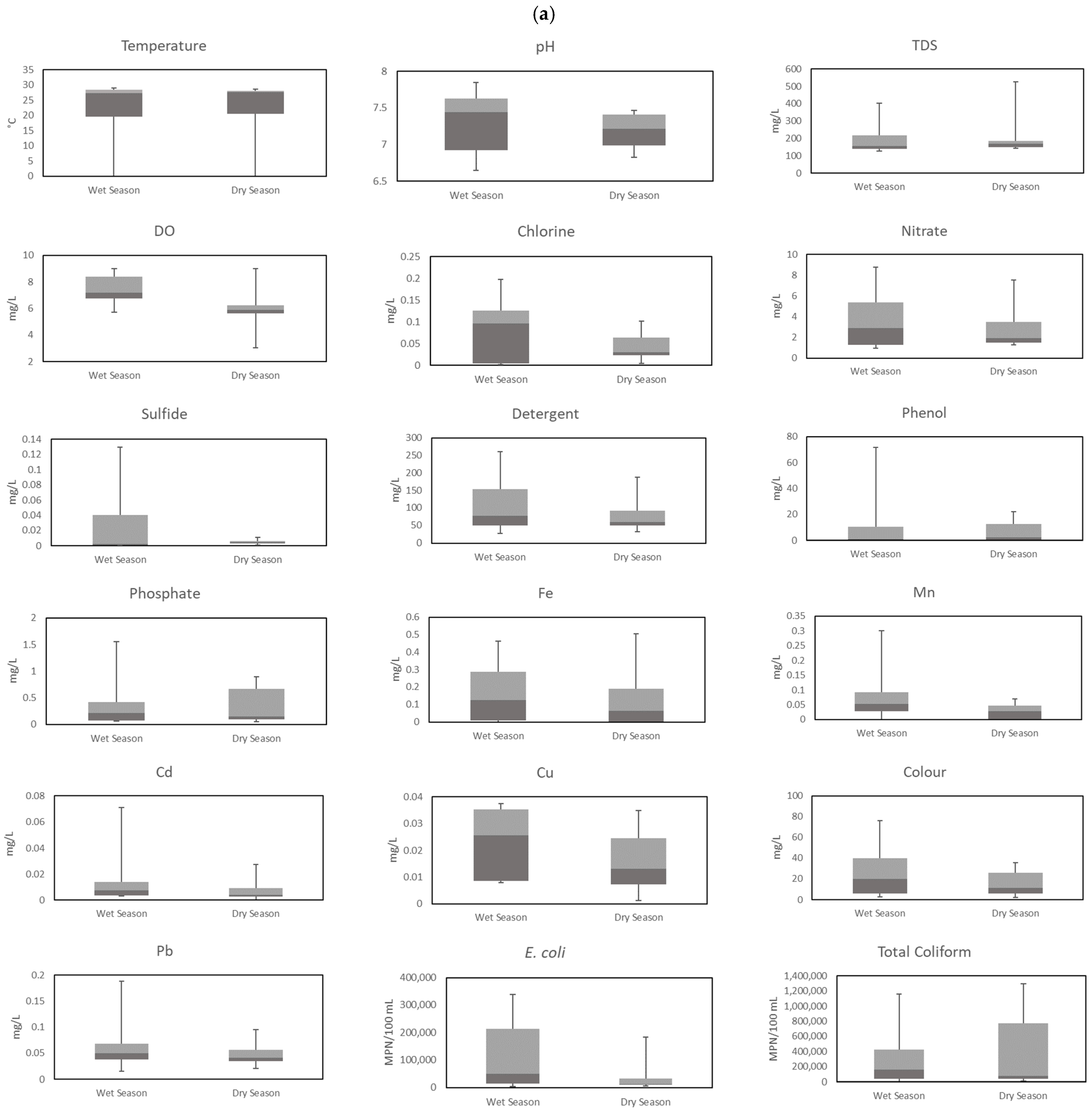
3.1. Temporal Analysis of the Opak Sub-Watershed’s Water Quality

The temporal trend of the Opak sub-watershed was classified based on the season from 2013 to 2020. As explained by the Meteorological, Climatological, and Geophysical Agency (BMKG) of Yogyakarta Province [30,48], in Table 2, the wet season (or rainy season) peaked in February/March and the peak of the dry season was in September/October. Furthermore, water quality parameters were clustered into a gradual decline and rising in median parameters from the wet to dry season. The trend of decreasing median parameters from wet season to dry season includes temperature, pH, TDS, DO, chlorine, nitrate, sulfide, detergent, phenol, phosphate, Fe, Mn, Cd, Cu, Pb, colour, E. coli, and Total Coliform. On the other hand, there is the increasing concentration of water quality parameters, such as TSS, BOD5, COD, nitrite, ammonia, oil and grease, and zinc (Zn).
It can be seen in Figure 2 that the temperature of water in the Opak sub-watershed was not dissimilar between wet and dry seasons. The median of both seasons ranged from 27.36–27.66 °C. The minimum temperature was reported in the wet season of 26.0 °C and the maximum temperature in the dry season was 28.6 °C. Furthermore, dissolved oxygen (DO) levels were at their highest during the rainy season, while during the dry season, concentration was the lowest.
In tropical countries, surface water quality has been shown to shift seasonally in response to changes in temperature and rainfall [49,50,51]. In Indonesia, the difference between low and high precipitation during the dry and wet seasons impacted the water quality of the watershed significantly [52,53]. Subsequently, TDS and TSS parameters for solids in river water exhibited the same pattern in both seasons. The TSS value was higher than the TDS during the dry season. It was thought that suspended particles make up most solids in the Opak sub-watershed, making it difficult for particles to settle even in the dry season. The sources of suspended solids came from erosion and runoff, human pollution, algae, and sediment disruption. The sediment and the Opak sub-watershed were also contributed to via volcanic activity from Mount Merapi [54].
Based on DO measurement results, previous research shows that rainfall had a positive connection with DO [55,56,57,58]. Rainwater entering the riverbanks allowed aeration of the water body that increased the river current and speed flow. The levels of BOD5 and COD in river water of the Opak sub-watershed were inversely related to this. BOD5 and COD levels in the wet season were lower than in the dry season due to the dilution process. The high percentage of vegetation land (32.2%) in the overall watershed produced a lot of organic matter from decaying leaves and wood transported by water run-off into the water body so that BOD5 level was high [59,60,61]. Furthermore, wastewater incredibly contributed to the rise of BOD5 and COD values, typically in organic matter from settlement point sources.
Several parameters primarily found in industrial wastewater, such as chlorine, sulfide, and phenols, were reported to have a decreasing trend from wet to dry season. Similarly, the elements N (nitrate) and P (phosphate) in the waters followed a similar pattern, with those concentrations being higher in the wet season than in the dry season. According to Ling et al., pollutant matters dissolved and accumulated at the bottom of the sediment river were released quickly and well mixed within the water column during the wet season [62,63]. Furthermore, a significant volume of inflow following heavy rainfall encourages mixing and disrupts reservoir stratification. In the nitrogen cycle, the level of nitrate was opposite to nitrite and ammonia parameters. Nitrite was the only form of partially oxidized nitrogen that formed during ammonia oxidation to nitrate and lasted only a short period [64,65,66,67]. Then, denitrification occurred at low levels of dissolved oxygen-producing ammonia. These facts are associated with the data collected in the Opak sub-watershed that the depletion of dissolved oxygen levels during the dry season generated lifted ammonia levels.
Almost all metals, both essential (Fe, Mn, and Cu) and non-essential (Cd and Fb), decreased from wet to dry season. Anthropogenic and industrial activities and natural phenomena contributed to the metal sources inside the water body. Metals could be in water structures as colloids, particles, or dissolved or adsorbed to sediment [68]. Dissolution and precipitation processes during the rainy season played a role in metal transport in aquatic environments [69,70]. Thus, metals stored in the mountain rock or soil layers that originated in a volcano might be easily washed off during rainfall and enter river bodies. The metal that has been deposited in the sediment originated from domestic, industrial, and agricultural activities.
Water contained fecal contamination indicators that were critical for determining the quality of the water. Total coliforms and E. coli were the most extensively used bacteriological assays to detect harmful bacteria in animal and human feces [71]. In this study, the highest total coliforms and E. coli in the dry season were 1,296,125 MPN/100 mL and 183,500 MPN/100 mL, respectively. Their quantities at all monitoring stations were negatively under the most minimum water quality criteria. The presence of these bacteria in the Winongo River was highly concerning to residents around the Opak Sub-watershed. The health risks had increased due to the chance of their exposure to these microorganisms. The wet season was expected to be polluted by fecal coliforms due to overflows of its banks. The water run-off that had been contaminated by animal and human excrement flew into the water body.
Nevertheless, the findings revealed contrary results. It was clear that the microenvironment influenced their appearance or reappearance and the number of coliforms present [72,73,74]. Changes in the number and diversity of bacteria were observed as the season altered. When water temperatures rose above 15 °C, the existence of total coliforms increased considerably. This was assumed since the temperature was a significant controlling element in bacterial growth.

3.2. Spatial Analysis of the Opak Sub-Watershed’s Water Quality

In the spatial analysis data, water quality parameters are divided into two groups, i.e., the trend of increasing and random median parameters from upstream, middle stream, and downstream, respectively. Random trends sometimes mean the highest concentration accumulated on the middle stream, and occasionally they fluctuated among three sampling points. Overall, water parameters in the Opak sub-watershed climbed up from upstream to downstream, such as temperature, TDS, TSS, COD, nitrate, nitrite, sulfide, ammonia, detergent, phosphate, Fe, Mn, Cd, Zn, Cu, colour, E. coli, and total coliform. That aside, pH, BOD5, phenol, oil and grease reached the largest concentration in the middle stream. Chlorine and Pb levels shifted for every observation point. Then, dissolved oxygen (DO) concentration steadily decreased from upstream to downstream.
As shown in Figure 3, the temperature between the middle stream (MD2) and downstream (DW3) is invariable, around 28 °C. Moreover, TDS gradually climbed up to the third monitoring station, whereas the TSS value remained stable. Furthermore, several parameters showed a random trend, such as chlorine, phenol, Pb, oil, and grease. The chlorine and Pb levels peaked in the last stream while phenol, oil, and grease surged in the second stream of the Opak sub-watershed.
The upstream (UP1) is 3 °C cooler than the others, which is different from the two sites before. The temperature of the surrounding air had a significant impact on the temperature of the river water. Warmer urban surfaces caused temperature surges in streams. According to the landscape of the study area, MD2 and DW3 is located in the tight, densely population area. Land-use changes linked to urbanization lead to changes in the temperature regime of the air in cities, resulting in urban heat islands [75,76,77]. Furthermore, domestic residential wastewater was a pivotal contributor to rising river water temperatures [78,79,80].
The sources of solids inside the water column were dominated by outside factors, such as erosion, run-off, flooding, etc. In UP1, the riverbanks’ vegetation could hold the soil, so it was not be carried away by the water flow. The combined impacts of leaves, stems, roots, and litter allowed plants to intercept rainfall and control surface run-off, thus fulfilling the function of soil and water conservation [10,81,82,83,84]. Furthermore, TSS concentration was influenced by the material derived from land carried by river flows [85,86,87].
By comparing BOD5 and COD, the median of BOD5 rose from UP1 to MD2, then fell as it entered DW3. Generally, the DO level is constantly depleted in the three monitoring points. On the contrary, BOD5 and COD increased. A similar phenomenon happened for other parameters, such as NO2, NO3, NH3, PO4 and detergent. A lot of dissolved oxygen is used inside the water body. The oxidation process of those matters rapidly occurs and generates a high concentration of not only BOD5 and COD but also N and P elements. Commonly, organic matters originated from settlements and industrial activities. In addition, the MD2 and DW3 were circled by several kinds of home industries, such as tofu industries. Previous research shows that approximately five tofu home industries did not treat their wastewater and discharged it directly into the river [88]. Through observing around the study area, the numerous sewer pipes flew directly to the water body of the Winongo river.
The presence of phenolics in water could be attributed to the deterioration or decomposition of natural organic materials in the water and the discharge of industrial and residential wastewater and runoff from agricultural lands [89]. On the other hand, chlorine was also used in wastewater treatment plants and swimming pools as a disinfectant, as a bleaching agent in textile manufacturers and paper mills, and as an element in many laundry bleaches [90,91]. Both phenol and chlorine were poisonous to aquatic organisms even at deficient levels.
Furthermore, as one of the heavy metals, Pb possessed a bizarre phenomenon in this study. All the metals concentration, substantial and non-substantial, steadily increasing from UP1 to DW3, except Pb. The level of Pb was high in two monitoring locations, upstream and downstream, 0.03 and 0.05 ppm, respectively. In the middle stream, Pb concentration jumped down to 0.02 ppm. It was assumed that Pb metal was easier to settle and bond to other elements due to the affinity sequence; therefore, the concentration of Pb did not accumulate in the following sampling point. The source of Pb in the upstream river was river rocks, and volcanic activity carried downstream by water currents. Consequently, the concentrations of Pb in each stream was different. Despite this, the majority of the Pb in the downstream came from human activities.
Based on spatial analysis, the microbial parameters exceed the water quality standard for all monitoring locations of the Opak sub-watershed. The presence of high levels of coliform can be caused by various reasons, particularly sanitation issues such as the usage of septic tanks and the distance between water sources and pollutants. Furthermore, coliform bacteria from the digestive systems of human and animal bodies could be released by organism generated waterborne illness through surface water [92,93,94]. Before flowing into the MD2, the Opak sub-watershed flows through the agricultural land. It assumed that the high E. coli and total coliform number were caused by mammal feces-based fertilizer. Subsequently, E. coli and total coli bacteria parameters originated from the black water of domestic activity [95,96,97]. Water quality characteristics of Winongo river as Opak sub-watershed, in 2012–2014 was classified as heavily polluted [98,99,100]. It was indicated by BOD5, COD, Pb, and total coliform exceeding the second class of water quality standard named Pergub DIY No. 20/2008.

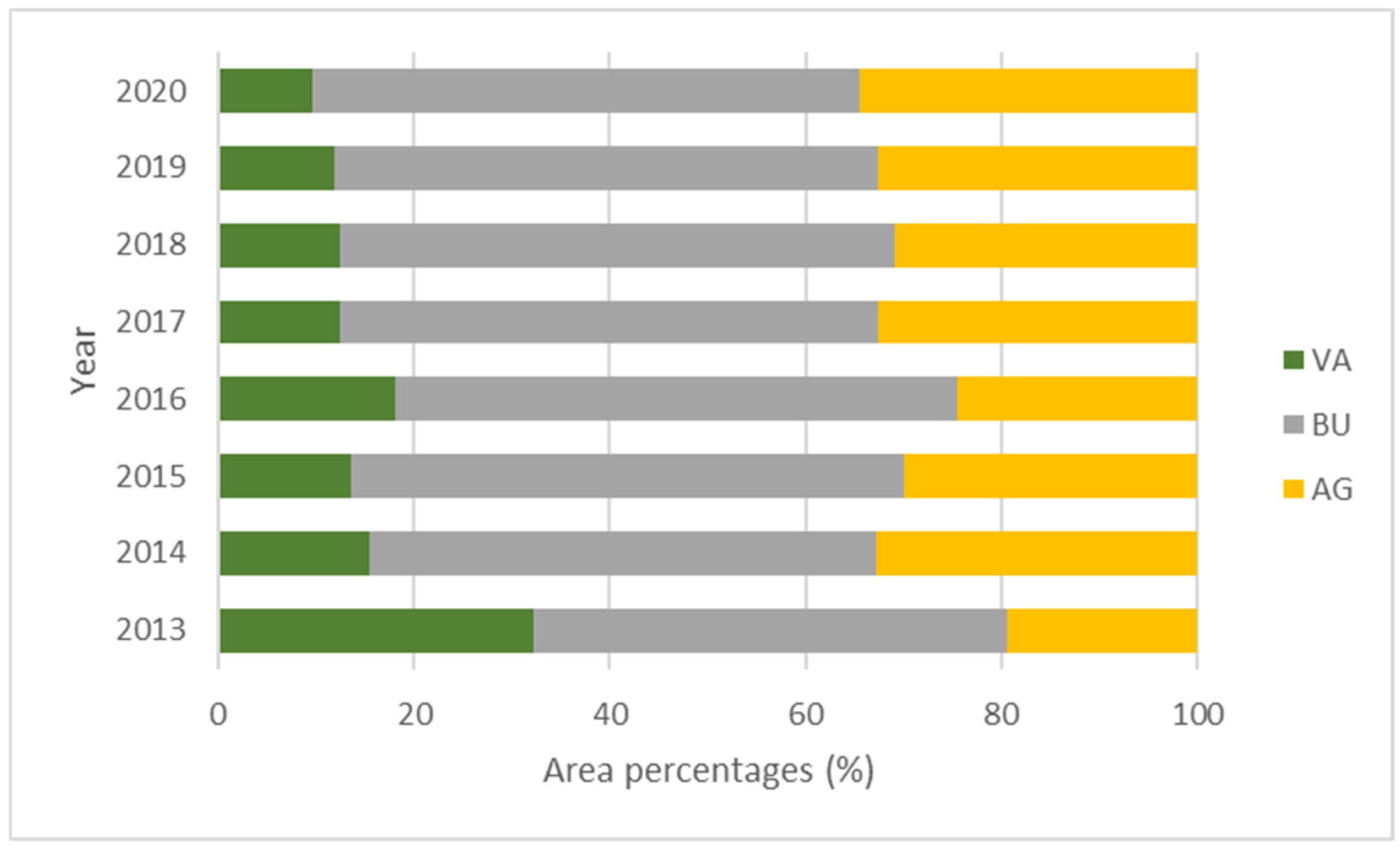
3.3. Land Use Impact to Water Quality

The Landsat satellite captured the land use images and the Opak sub-watershed for 2013–2020. Figure 4 shows the proportion of land use in three categories and three river zones. Significantly, vegetation land decreased from 2013 to 2014 in all stream areas, and then it was the relatively stable condition under 30% of coverage area up to 2020. Complementary to this, building area was dominated more than 60% in the middle and downstream. Moreover, the agriculture area was the most fluctuated trend in the upstream zone. The sizeable vacant space and cooler altitude temperature upstream were utilized for seasonal cultivated vegetation, such as paddy, corn, potatoes, etc. So that the percentages of agriculture area were up and down ranging from 20–45% for seven years, it can be seen in river zone, and upper area exhibited different pattern compared to middle and down zones. In upstream, natural vegetation and building had contrary trend, while crop area varies changed. On the other hand, settlement and non-settlement areas reached more than 80% and about 60% in the middle and downstream.
To elaborate on the quantity of land use in the Opak sub-watershed and image data, Figure 5 shows the visual land cover from 2013 to 2020. The greenest area in the upstream (UP1) was significantly changed in 2013–2014. In the middle (MD2), it constantly exposed red areas dominated by buildings. The combination between building and agriculture are located in the last stream (DW3). The impact of land use on the water quality in the Opak sub-watershed was calculated by Pearson correlation coefficient (r). Table 3 exhibits the most significant relation (r > 0.6) between two variables, land use and water quality parameters, in the upper, middle, and downstream.
The results of land cover mapping supported by another research that the land cover of Winongo river, part of Opak sub-watershed, was geographically variable. The woodland and plantation regions were dominated the upstream basin [101]. Besides, in the city of Yogyakarta, settlements spots were the most common land cover. Furthermore, Paddy fields mostly covered Bantul and Sleman regencies. In UP1, sulfide, ammonia, and some metals (Mn, Zn, Pb) strongly correlated. The green area (VA) upstream owned the positive correlation (0.876) with sulfide. In the natural condition, sulfide was formed by the decomposing process of organic matter, such as plant material [102,103]. Additionally, semi and non-permanent buildings in the upstream associated positively to Zn and Pb parameters, 0.738 and 0.765, respectively. Complementary to this, ammonia (−0.821) and Mn (−0.748) had a strong negative correlation between structured area (AB) and organic and metal contaminants. The significance of r values in the middle stream was not different from the previous watershed part that was still sulfide, ammonia, and metals parameters. The run-off accumulation of sulfide sources from upstream areas, vegetation, and agriculture generated a high correlation coefficient, 0.865 and −0.718, respectively. Not only from plant decaying but also dissolved evaporite mineral from fertilizer and soil sulfates become the other sources of sulfide [104,105,106].
The dense population and various home industries (AB) contributed to metal contamination in the middle stream. In the last part of the Opak sub-watershed, numerous water quality parameters exhibited high correlation, such as BOD5, detergent, phenol, Cd, Pb, and Cu. BOD5 possessed a remarkable correlation up to 0.886 of VA and −0.936 of AB. It was expected from the organic compound degradation process that originated domestic wastewater [107,108,109]. Phenol was found strong relation with VA (0.713) and AB (−0.816) that indicated pollution from industrial, agricultural, and home sources. Cd and Pb showed a significant correlation with VA and AB. Besides industrial sources, Cd and Pb in the water body came from the atmosphere [110,111,112]. The fuels used from the engine of transportation emitted to the atmosphere, and during the rainy season was dropped into surface water and was expected through run-off from open space.
More importantly, an unexpected correlation was found, for example, between Cd and Pb and vegetation (0.837 and 0.752, respectively). Such strong correlation was not found in previous research [22] so that further investigations are required to explain the association between heavy metal and vegetation. Another essential point, the determination of VA (vegetation area), is needed to be clarified. It was supported by previous finding that cadmium became an issue combining phosphorus fertilizers [113]. Replanting or revegetation in such blank areas using fertilizer could contribute heavy metal sources through run-off into riverbanks.

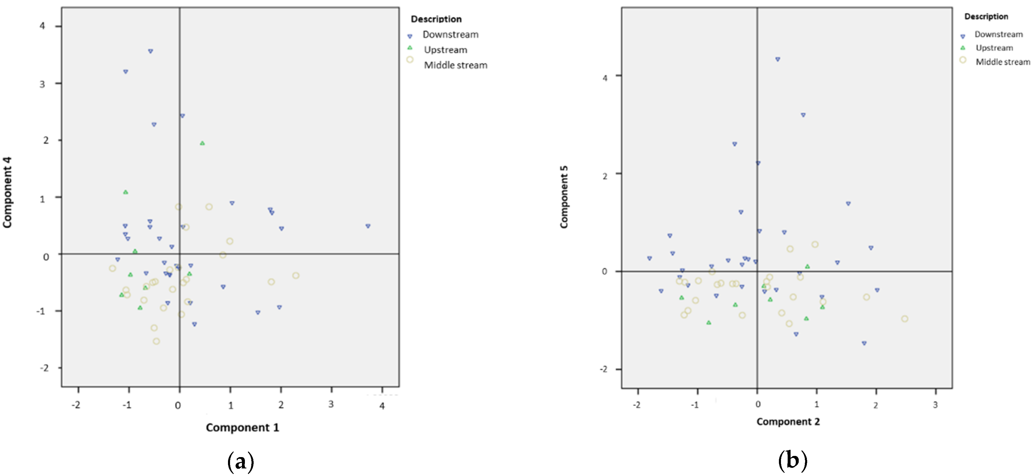
3.4. Principal Component Analysis (PCA) of Pollution Source

Principal component analysis (PCA) was used to determine the pollution sources in the Opak sub-watershed. To validate the statistical requirement of PCA analysis, preliminary tests, such as KMO, Bartlett, and anti-image matric tests, were done. Four out of 25 water quality parameters, i.e., TSS, chlorine, COD, and sulfide, were eliminated from the analysis due to over 0.5 anti-image correlation. Subsequently, six components were obtained from the total variance calculation. The eigenvalue of those components should be more than 1.0. The sampling adequacy of the Kaiser-Meyer-Oikin (KMO) test showed a value of 0.628 to continue the analysis. Furthermore, by calculating the next step of the rotated component matrix, BOD5 was ineligible (<0.5) so that the twenty remaining parameters are re-extracted and displayed in Table 4.
The source of pollution was represented by six extracted components with a total variance of 69.313% (Table 3). The first component, 21.393% of the total variance, consisting of temperature, TDS, detergent, E. coli, and total coliform, described domestic activities and human fecal contamination. As identical sub-watershed in Yogyakarta Province, Code River showed a different pattern with the present study that COD and BOD5 [21] classified the main organic compounds. The second, fourth, and sixth components, 15.809%, 8.671%, and 5.778% of the total variance, respectively, defined an industrial characteristic regarding Mn, Cd, Zn, Fe, Pb, Cu, pH, phenol, and oil and grease. Additionally, the third (10.468%) and fifth (7.194%) components portrayed the contaminant from agriculture activities correlating with nitrate, nitrite, phosphate, ammonia, and DO parameters.
The selected components were loaded in the scatter plot imagined in Figure 6 for each location of the sub-watershed. In Figure 6a, the dots are centered in negative value both an x-axis and y-axis tend to disperse in a horizontal line (Component 1). The purple triangle (downstream), the green triangle (upstream), and the brown circle (middle stream) were represented by organic contaminants from domestic activities. It can be seen in Figure 6b, the points are more aligned with the x-axis than the y-axis, not only in the positive value but in the negative values. Most middle and downstream scatters represented component 2 (industrial activities) since the heavy metal was the primary source. As well as Figure 6c also presented the sources of organic contaminant from oil and grease and inorganic compound, cuprum (component 6). In addition, Figure 6d explains the organic compound from agriculture activities. The finding correlated with the cropland use in the upstream and lowest stream. Significantly, the downstream showed a more dispersed pattern into x-axis (component 3) and y-axis (component 5) than two others.
The presence of E. coli and total coliform in the water indicated that the water had been contaminated by human feces or animal waste [90]. The animal waste potentially originated from organic fertilizer used in an agricultural are, while the human feces were from black water contaminating the surface water. By observing the riverbank area of the Opak sub-watershed, several home industries (building area) were operated surrounding the water body, for instance, a jewelry plating home industry. The outlet of the kinds of industries was used to generate a point source of surface water contaminant. Based on land-use findings in the middle and downstream, the rapid settlements, hotels, restaurants, laundries, and so on, produced the domestic wastewater that is often directly discharged into the water body. Components 3 and 5 described nitrate, nitrite, phosphate, and ammonia parameters. The impact of agricultural activities would produce solid runoff from fertilizer containing nitrate and phosphate. The compounds flew into surface water and caused the rise in nutrients inside the river [114,115,116].

4. Conclusions

This study investigated the relationship between land use and river water quality in the Opak sub-watershed represented on Winongo River, Indonesia. The temporal (seasonal time) and spatial analysis were employed based on multivariate and GIS methods. By utilizing PCA analysis, three main kinds of pollutant sources were obtained, such as domestic, industrial, and agricultural activities that contributed and influenced the variance of river water quality. The different land uses exhibited a significant correlation of contaminant sources that ranged between 0.712 and 0.936 (0.05 significance level, p < 0.05). This study also found that the water quality trend based on the concentration value has increased for all parameters spatially. The water quality tended to decline from upstream to downstream. While the seasonal trend of water quality fluctuated, this explained the local climate’s contribution to contaminant spreading and degrading. The findings of this study can be expanded to guide water quality management in the Opak sub-watershed and assist the stakeholders in selecting wastewater pollution control actions.

Author Contributions

Conceptualization: W.B. and A.A.A.; methodology: A.A.A.; software: A.A.A.; validation: W.B., A.A.A., R.J., A.Y. and S.R.; formal analysis: A.A.A.; investigation: A.A.A.; resources: W.B. and A.A.A.; data curation: A.A.A., R.J. and S.R.; writing—original draft preparation: W.B. and A.A.A.; writing—review and editing: W.B., A.A.A., R.J. and A.Y.; visualization: A.A.A., R.J., A.Y. and S.R.; supervision: W.B.; project administration: A.A.A.; funding acquisition:pted W.B. and A.A.A. All authors have read and agreed to the published version of the manuscript.

Funding

This research received no external funding.

Institutional Review Board Statement

Not applicable.

Informed Consent Statement

Not applicable.

Data Availability Statement

The data presented in this study are available on request from the corresponding author. The data are not publicly available due to university’s policy.

Acknowledgments

The authors thank Direktorat Pengembangan Akademik, Universitas Islam Indonesia for financial support for publishing this article.

Conflicts of Interest

The authors declare no conflict of interest.

References

  1. Permatasari, P.A.; Setiawan, Y.; Khairiah, R.N.; Effendi, H. The Effect of Land Use Change on Water Quality: A Case Study in Ciliwung Watershed. In Proceedings of the IOP Conference Series: Earth and Environmental Science, Shanghai, China, 19–22 October 2017; IOP Publishing: Bogor, Indonesia, 2017; Volume 54, p. 012026. [Google Scholar]
  2. Brontowiyono, W. Sustainable Water Resources Management with Special Reference to Rainwater Harvesting—Case Study of Karta-ManTul; Universitat Karlsruhe: Java, Indonesia, 2008. [Google Scholar]
  3. Statistics of Daerah Istimewa Yogyakarta. Provinsi Daerah Istimewa Yogyakarta Dalam Angka 2021 [Daerah Istimewa Yogyakarta Province in Figures 2021]; Statistics of Daerah Istimewa Yogyakarta: Yogyakarta, Indonesia, 2021. [Google Scholar]
  4. Mahzum, M.M. Water Resources Availability Analysis and Brantas Sub-Watershed Conservation Effort the Upper of The Batu City Area; Sepuluh Nopember Institute of Technology Surabaya: Surabaya, Indonesia, 2015. [Google Scholar]
  5. Kementrian Lingkungan Hidup dan Kehutanan. Petunjuk Teknis Restorasi Kualitas Air (Technical Instruction for Water Quality Restoration); Kementrian Lingkungan Hidup dan Kehutanan: Jakarta, Indonesia, 2017. [Google Scholar]
  6. Universitas Gadjah Mada 119 Sumber Mata Air Di Kulon Progo Terancam Hilang [119 Springs in Kulon Progo Are in Danger of Losing]. Available online: https://www.ugm.ac.id/id/berita/340-119-sumber-mata-air-di-kulon-progo-terancam-hilang (accessed on 12 January 2022).
  7. Budianto, A. Lingkungan Rusak, Puluhan Mata Air Di Kota Bandung Kritis [Damaged Environment, Dozens of Springs in Bandung City Are Critical]. Available online: https://jabar.inews.id/berita/lingkungan-rusak-puluhan-mata-air-di-kota-bandung-kritis (accessed on 1 February 2022).
  8. Tahiru, A.A.; Doke, D.A.; Baatuuwie, B.N. Effect of Land Use and Land Cover Changes on Water Quality in the Nawuni Catchment of the White Volta Basin, Northern Region, Ghana. Appl. Water Sci. 2020, 10, 198. [Google Scholar] [CrossRef]
  9. Camara, M.; Jamil, N.R.; Bin Abdullah, A.F. Impact of Land Uses on Water Quality in Malaysia: A Review. Ecol. Processes 2019, 8, 10. [Google Scholar] [CrossRef]
  10. Hua, A.K. Land Use Land Cover Changes in Detection of Water Quality: A Study Based on Remote Sensing and Multivariate Statistics. J. Environ. Public Health 2017, 2017, 7515130. [Google Scholar] [CrossRef] [PubMed] [Green Version]
  11. James, T. Changes in Land Use Land Cover (LULC), Surface Water Quality and Modelling Surface Discharge in Beaver Creek Watershed, Northeast Tennessee and Southwest Virginia; East Tennessee State University: East Tennessee, TN, USA, 2020. [Google Scholar]
  12. Tripathi, M.; Singal, S.K. Use of Principal Component Analysis for Parameter Selection for Development of a Novel Water Quality Index: A Case Study of River Ganga India. Ecol. Indic. 2019, 96, 430–436. [Google Scholar] [CrossRef]
  13. Lee, J.Y.; Yang, J.S.; Kim, D.K.; Han, M.Y. Relationship between Land Use and Water Quality in a Small Watershed in South Korea. Water Sci. Technol. 2010, 62, 2607–2615. [Google Scholar] [CrossRef] [PubMed] [Green Version]
  14. Khaledian, Y.; Ebrahimi, S.; Basatnia, N.; Zeratpisheh, M.; Ghafarpour, A. Evaluation Land Use Changes and Anthropogenic Influences on Surface Water Quality by Principal Component Analysis, Northern Iran. In Proceedings of the 1st International Conference on Environmental Crisis and Its Solutions, Kish Island, Iran, 13–14 February 2013. [Google Scholar]
  15. Bahar, M.M.; Ohmori, H.; Yamamuro, M. Relationship between River Water Quality and Land Use in a Small River Basin Running through the Urbanizing Area of Central Japan. Limnology 2008, 9, 19–26. [Google Scholar] [CrossRef]
  16. Maghfiroh, M.; Novianti, H.; Lukman; Nurtjahya, E. Bacterial Indicators Reveal Water Quality Status of Rangkui River, Bangka Island, Indonesia. IOP Conf. Ser. Earth Environ. Sci. 2019, 380, 12008. [Google Scholar] [CrossRef]
  17. Nugraha, W.D. Analisis Pengaruh Hidrolika Sungai Terhadap Transport BOD Dan DO Dengan Menggunakan Software QUAL2E (Studi Kasus Di Sungai Kaligarang, Semarang). J. Presipitasi 2007, 2, 66–70. [Google Scholar] [CrossRef]
  18. Indriyani, K.; Hasibuan, H.; Gozan, M. Impacts of Land Use and Land Use Change in River Basin to Water Quality of Cirarab River, Indonesia. In Proceedings of the 1st International Conference on Environmental Science and Sustainable Development ICESSD 2019, Jakarta, Indonesia, 22–23 October 2019; Saiya, H.G., WeziaSulthonudin, I.B., Putra, G.A.Y., Astuti, D., Eds.; European Alliance for Innovation (EAI): Jakarta, Indonesia, 2020. [Google Scholar]
  19. Suharyo, Y. Analisis Hubungan Tata Guna Lahan Terhadap Kualitas Air Parameter Kimia (BOD, COD, Amonia) Di Daerah Aliran Sungai Opak, Yogyakarta [Analysis of the Relationship between Land Use and Water Quality Chemical Parameters (BOD, COD, Ammonia) in the Opak River; Universitas Islam Indonesia: Yogyakarta, Indonesia, 2019. [Google Scholar]
  20. Hamid, N. Monitoring Bakteri Escherichia Coli Pada Air Sumur Gali Di Sekitar Sungai Code (Studi Kasus: Kelurahan Tegalpanggung Kec. Danurejan Yogyakarta) [Monitoring Escherichia Coli Bacteria in Dug Well Water around the Code River (Case Study: Tegalpanggung, Danu)]; Universitas Islam Indonesia: Yogyakarta, Indonesia, 2007. [Google Scholar]
  21. Munawar, M. Study of the Water Quality of the Code River, Special Region of Yogyakarta on the Basis of Differences in Land Use; Universitas Gadjah Mada: Yogyakarta, Indonesia, 2011. [Google Scholar]
  22. Pratama, M.A.; Immanuel, Y.D.; Marthanty, D.R. A Multivariate and Spatiotemporal Analysis of Water Quality in Code River, Indonesia. Sci. World J. 2020, 2020, 8897029. [Google Scholar] [CrossRef] [PubMed]
  23. Ujianti, R.M.D.; Anggoro, S.; Bambang, A.N.; Purwanti, F. Water Quality of the Garang River, Semarang, Central Java, Indonesia Based on the Government Regulation Standard. J. Phys. Conf. Ser. 2018, 1025, 12037. [Google Scholar] [CrossRef] [Green Version]
  24. Taufiq, A.; Effendi, A.J.; Iskandar, I.; Hosono, T.; Hutasoit, L.M. Controlling Factors and Driving Mechanisms of Nitrate Contamination in Groundwater System of Bandung Basin, Indonesia, Deduced by Combined Use of Stable Isotope Ratios, CFC Age Dating, and Socioeconomic Parameters. Water Res. 2019, 148, 292–305. [Google Scholar] [CrossRef]
  25. Pemerintah Daerah Daerah Istimewa Yogyakarta. Rencana Kerja Pembangunan Daerah Provinsi Daerah Istimewa Yogyakarta 2016 [Regional Development Work Plan of Special Region of Yogyakarta Province 2016]; Pemerintah Daerah Daerah Istimewa Yogyakarta: Yogyakarta, Indonesia, 2015. [Google Scholar]
  26. Dinas Lingkungan Hidup Kabupaten Bantul. Laporan Akhir Konservasi Sungai Winongo 2020 [Final Report of Winongo River Conservation 2020]; Dinas Lingkungan Hidup Kabupaten Bantul: Bantul, Indonesia, 2020. [Google Scholar]
  27. Kartiko, H. Estimasi Sumber Pencemar Dan Beban Pencemar Sungai Winongo (Sub DAS Bagian Barat-Hilir) [Estimation of Pollution Sources and Contaminant Loads of The Winongo River (West-Downstream Sub-Watershed)]; Universitas Islam Indonesia: Yogyakarta, Indonesia, 2019. [Google Scholar]
  28. Prananda, E.G. Perencanaan Flood Early Warning System Di Sungai Winongo (Simulasi HEC-RAS) [Flood Early Warning System Planning in The Winongo River (HEC-RAS Simulation)]; Atma Jaya University: Yogyakarta, Indonesia, 2017. [Google Scholar]
  29. Despensary, A. Kajian Neraca Air: Studi Kasus Di Daerah Aliran Sungai Winongo Dan Gajahwong Daerah Istimewa Yogyakarta [Water Balance Study: A Case Study in the Winongo and Gajahwong Watersheds, Special Region of Yogyakarta]; Universitas Gadjah Mada: Yogyakarta, Indonesia, 2006. [Google Scholar]
  30. Statistics of Daerah Istimewa Yogyakarta Jumlah Curah Hujan Dan Hari Hujan Menurut Bulan Di D.I. Yogyakarta, 2019 [Amount of Precipitation and Number of Rainy Days by Month in D.I. Yogyakarta, 2019]. Available online: https://yogyakarta.bps.go.id/statictable/2020/06/15/93/jumlah-curah-hujan-dan-hari-hujan-menurut-bulan-di-d-i-yogyakarta-2019.html (accessed on 23 March 2021).
  31. Mawardi, I. Upaya Meningkatkan Daya Dukung Sumberdaya Air Pulau Jawa [Efforts to Increase the Carrying Capacity of Java’s Water Resources]. J. Teknol. Lingkung. 2008, 9, 98–107. [Google Scholar] [CrossRef] [Green Version]
  32. Mawardi, I. Kerusakan Daerah Aliran Sungai Dan Penurunan Daya Dukung Sumberdaya Air Di Pulau Jawa Serta Upaya Penanganannya [Damage to Watersheds and Decrease in Carrying Capacity of Water Resources in Java Island and Their Handling Efforts]. J. Hidrosfir Indones. 2010, 5, 1–11. [Google Scholar]
  33. Zulfahmi, Z.; Syam AS, N.; Jufriadi, J. Dampak Sedimentasi Sungai Tallo Terhadap Kerawanan Banjir Di Kota Makassar [Impact of Tallo River Sedimentation on Flood Vulnerability in Makassar City]. Plano Madani 2016, 5, 180–191. [Google Scholar] [CrossRef]
  34. Brontowiyono, W.; Kasam, K.; Ribut, L.; Ike, A. Strategi Penurunan Pencemaran Limbah Domestik Di Sungai Code DIY [Domestic Waste Pollution Reduction Strategy in Code DIY River]. J. Sains Teknol. Lingkung. 2013, 5, 36–47. [Google Scholar] [CrossRef] [Green Version]
  35. Susanti, P.D.; Miardini, A. The Impact of Land Use Change on Water Pollution Index of Kali Madiun Sub-Watershed. Forum Geogr. 2017, 31, 128–137. [Google Scholar] [CrossRef] [Green Version]
  36. Vandith, V.A.; Setiyawan, A.S.; Soewondo, P.; Putri, D.W. The Characteristics of Domestic Wastewater from Office Buildings in Bandung, West Java, Indonesia. Indones. J. Urban Environ. Technol. 2018, 1, 199–214. [Google Scholar] [CrossRef] [Green Version]
  37. Gurning, L.F.P.; Nuraini, R.A.T.; Suryono, S. Kelimpahan Fitoplankton Penyebab Harmful Algal Bloom Di Perairan Desa Bedono, Demak [Abundance of Phytoplankton Causes Harmful Algal Bloom in the Waters of Bedono Village, Demak]. J. Mar. Res. 2020, 9, 251–260. [Google Scholar] [CrossRef]
  38. Yogaswara, D. Distribusi Dan Siklus Nutrient Di Perairan Estuari Serta Pengendaliannya [Distribution and Cycle of Nutrients in Estuary Waters and Their Control]. Oseana 2020, 45, 28–39. [Google Scholar] [CrossRef]
  39. Nugroho, S.; Akbar, S.; Vusvitasari, R. Kajian Hubungan Koefisien Korelasi Pearson (r), Spearman-Rho (ρ), Kendall-Tau (τ), Gamma (G), Dan Somers (Dxy) [Study of Correlation between Pearson (r), Spearman-Rho (ρ), Kendall-Tau (τ), Gamma (G), and Somers (Dxy) Coefficients]. J. Gradien 2008, 4, 372–381. [Google Scholar]
  40. Ashoor, A.S.; Naji, A.A.K.K. Integrated Network of Pearson Correlation Coefficients, Kendall Tau, Spearman Rho and Its Impact on Disease, Health Indicators and Mortality Ratings in Babil Province BT. In Proceedings of the First International Conference on Mathematical Modeling and Computational Science, Pattaya, Thailand, 4 May 2021; Peng, S.-L., Hao, R.-X., Pal, S., Eds.; Springer: Singapore, 2021; pp. 83–96. [Google Scholar]
  41. Temizhan, E.; Mirtagioglu, H.; Mendes, M. Which Correlation Coefficient Should Be Used for Investigating Relations between Quantitative Variables? Am. Acad. Sci. Res. J. Eng. Technol. Sci. 2022, 85, 265–277. [Google Scholar]
  42. Bi, H.; Ni, Z.; Tian, J.; Jiang, C.; Sun, H.; Lin, Q. Influence of Lignin on Coal Gangue Pyrolysis and Gas Emission Based on Multi-Lump Parallel Reaction Model and Principal Component Analysis. Sci. Total Environ. 2022, 820, 153083. [Google Scholar] [CrossRef] [PubMed]
  43. Jansson, N.F.; Allen, R.L.; Skogsmo, G.; Tavakoli, S. Principal Component Analysis and K-Means Clustering as Tools during Exploration for Zn Skarn Deposits and Industrial Carbonates, Sala Area, Sweden. J. Geochem. Explor. 2022, 233, 106909. [Google Scholar] [CrossRef]
  44. Han, Y.; Song, G.; Liu, F.; Geng, Z.; Ma, B.; Xu, W. Fault Monitoring Using Novel Adaptive Kernel Principal Component Analysis Integrating Grey Relational Analysis. Process. Saf. Environ. Prot. 2022, 157, 397–410. [Google Scholar] [CrossRef]
  45. Hauben, M.; Hung, E.; Hsieh, W.-Y. An Exploratory Factor Analysis of the Spontaneous Reporting of Severe Cutaneous Adverse Reactions. Ther. Adv. Drug Saf. 2016, 8, 4–16. [Google Scholar] [CrossRef] [Green Version]
  46. Yang, Z.; Li, X.; Wang, Y.; Chang, J.; Liu, X. Trace Element Contamination in Urban Topsoil in China during 2000–2009 and 2010–2019: Pollution Assessment and Spatiotemporal Analysis. Sci. Total Environ. 2021, 758, 143647. [Google Scholar] [CrossRef]
  47. Constantin, C. Principal Component Analysis—A Powerful Tool in Computing Marketing Information. Bull. Transilv. Univ. Braşov. Ser. V Econ. Sci. 2014, 7, 27. [Google Scholar]
  48. Statistics D.I. Yogyakarta Curah Hujan per Bulan 2019 [Rainfall per Month 2019]. Available online: https://yogyakarta.bps.go.id/indicator/151/152/1/curah-hujan-per-bulan.html (accessed on 23 March 2021).
  49. Ling, T.Y.; Gerunsin, N.; Soo, C.L.; Nyanti, L.; Sim, S.F.; Grinang, J. Seasonal Changes and Spatial Variation in Water Quality of a Large Young Tropical Reservoir and Its Downstream River. J. Chem. 2017, 2017, 8153246. [Google Scholar] [CrossRef] [Green Version]
  50. Paul, M.J.; Coffey, R.; Stamp, J.; Johnson, T. A Review of Water Quality Responses to Air Temperature and Precipitation Changes 1: Flow, Water Temperature, Saltwater Intrusion. JAWRA J. Am. Water Resour. Assoc. 2019, 55, 824–843. [Google Scholar] [CrossRef]
  51. Tabari, H. Climate Change Impact on Flood and Extreme Precipitation Increases with Water Availability. Sci. Rep. 2020, 10, 13768. [Google Scholar] [CrossRef]
  52. Puspita, I.; Ibrahim, L.; Hartono, D. Pengaruh Perilaku Masyarakat Yang Bermukim Di Kawasan Bantaran Sungai Terhadap Penurunan Kualitas Air Sungai Karang Anyar Kota Tarakan (Influence of The Behavior of Citizens Residing in Riverbanks to The Decrease of Water Quality in The River of Karang). J. Mns. Lingkung. 2016, 23, 249–258. [Google Scholar] [CrossRef] [Green Version]
  53. Raharjo, I.; Zulkarnain, I.; Suprapto, S. Pengaruh Curah Hujan Terhadap Kualitas Air Sungai Way Kuripan Sebagai Sumber Air Baku Perusahaan Daerah Air Minum (PDAM) Way Rilau [The Effect of Rainfall on the Water Quality of the Way Kuripan River as a Source of Raw Water for the Way Rilau Regional Dr. J. Ilm. Tek. Pertan.-TekTan 2018, 5, 77–85. [Google Scholar] [CrossRef]
  54. Napsiah, N. Tindakan Warga Merapi Pascaerupsi Menjaga Daerah Tangkapan Air [The Actions of Merapi Residents After the Eruption to Protect the Catchment Area]. J. Penelit. Kesejaht. Sos. 2016, 15, 329–336. [Google Scholar] [CrossRef]
  55. Muñoz, H.; Orozco, S.; Vera, A.; Suárez, J.; García, E.; Neria, M.; Jiménez, J. Relación Entre Oxígeno Disuelto, Precipitación Pluvial y Temperatura: Río Zahuapan, Tlaxcala, México [Relationship between Dissolved Oxygen, Rainfall and Temperature: Zahuapan River, Tlaxcala, Mexico]. Tecnol. Cienc. Agua 2015, 6, 59–74. [Google Scholar]
  56. Liu, M.; Zhang, Y.; Shi, K.; Zhang, Y.; Zhou, Y.; Zhu, M.; Zhu, G.; Wu, Z.; Liu, M. Effects of Rainfall on Thermal Stratification and Dissolved Oxygen in a Deep Drinking Water Reservoir. Hydrol. Processes 2020, 34, 3387–3399. [Google Scholar] [CrossRef]
  57. Valappil, N.K.M.; Viswanathan, P.M.; Hamza, V. Chemical Characteristics of Rainwater in the Tropical Rainforest Region in Northwestern Borneo. Environ. Sci. Pollut. Res. 2020, 27, 36994–37010. [Google Scholar] [CrossRef]
  58. Zhi, W.; Feng, D.; Tsai, W.-P.; Sterle, G.; Harpold, A.; Shen, C.; Li, L. From Hydrometeorology to River Water Quality: Can a Deep Learning Model Predict Dissolved Oxygen at the Continental Scale? Environ. Sci. Technol. 2021, 55, 2357–2368. [Google Scholar] [CrossRef] [PubMed]
  59. Kurniawati, P.; Gusrianti, R.; Dwisiwi, B.B.; Purbaningtias, T.E.; Wiyantoko, B. Verification of Spectrophotometric Method for Nitrate Analysis in Water Samples. AIP Conf. Proc. 2017, 1911, 20012. [Google Scholar] [CrossRef] [Green Version]
  60. Susilowati, S.; Sutrisno, J.; Masykuri, M.; Maridi, M. Dynamics and Factors That Affects DO-BOD Concentrations of Madiun River. AIP Conf. Proc. 2018, 2049, 20052. [Google Scholar] [CrossRef]
  61. Anggraini, N.; Herdiansyah, H. COD Values for Determining BOD5 Dilution Factor in Faecal Sludge Waste—Case Study on the Duri Kosambi Faecal Sludge Treatment Plant in DKI Jakarta Province. AIP Conf. Proc. 2019, 2120, 40038. [Google Scholar] [CrossRef]
  62. Ling, T.Y.; Lee, T.Z.E.; Nyanti, L. Phosphorus in Batang Ai Hydroelectric Dam Reservoir, Sarawak, Malaysia. World Appl. Sci. J. 2013, 28, 1348–1354. [Google Scholar] [CrossRef]
  63. Ling, T.Y.; Gerunsin, N.; Soo, C.L.; Lee, N.; Sim, S.F.; Grinang, J. Nutrient Level of a Young Tropical Hydroelectric Dam Reservoir in Sarawak, Malaysia. Borneo J. Resour. Sci. Technol. 2018, 8, 14–22. [Google Scholar] [CrossRef] [Green Version]
  64. Sawyer, C.; McCarty, P.; Parkin, G. Chemistry for Environmental Engineering and Science, 5th ed.; McGraw-Hill Education: New York, NY, USA, 2002. [Google Scholar]
  65. Zhu, X.; Burger, M.; Doane, T.A.; Horwath, W.R. Ammonia Oxidation Pathways and Nitrifier Denitrification Are Significant Sources of N2O and NO under Low Oxygen Availability. Proc. Natl. Acad. Sci. USA 2013, 110, 6328–6333. [Google Scholar] [CrossRef] [Green Version]
  66. Kleerebezem, R.; Lücker, S. Cyclic Conversions in the Nitrogen Cycle. Front. Microbiol. 2021, 12, 622504. [Google Scholar] [CrossRef]
  67. Soler-Jofra, A.; Pérez, J.; van Loosdrecht, M.C.M. Hydroxylamine and the Nitrogen Cycle: A Review. Water Res. 2021, 190, 116723. [Google Scholar] [CrossRef]
  68. Weiner, E.R. Nutrients and Odors: Nitrogen, Phosphorus, and Sulfur. In Applications of Environmental Aquatic Chemistry: A Practical Guide; CRC Press: Boca Raton, FL, USA, 2013; pp. 133–180. [Google Scholar]
  69. Abdel-Ghani, N.T.; Elchaghaby, G.A. Influence of Operating Conditions on the Removal of Cu, Zn, Cd and Pb Ions from Wastewater by Adsorption. Int. J. Environ. Sci. Technol. 2007, 4, 451–456. [Google Scholar] [CrossRef] [Green Version]
  70. Oladoye, P.O. Natural, Low-Cost Adsorbents for Toxic Pb(II) Ion Sequestration from (Waste)Water: A State-of-the-Art Review. Chemosphere 2022, 287, 132130. [Google Scholar] [CrossRef]
  71. Muniz, J.N.; Duarte, K.G.; Ramos Braga, F.H.; Lima, N.S.; Silva, D.F.; Firmo, W.C.A.; Batista, M.R.V.; Silva, F.M.A.M.; Miranda, R.d.C.M.; Silva, M.R.C. Limnological Quality: Seasonality Assessment and Potential for Contamination of the Pindaré River Watershed, Pre-Amazon Region, Brazil. Water 2020, 12, 851. [Google Scholar] [CrossRef] [Green Version]
  72. Yadav, N.; Singh, S.; Goyal, S.K. Effect of Seasonal Variation on Bacterial Inhabitants and Diversity in Drinking Water of an Office Building, Delhi. Air Soil Water Res. 2019, 12, 1–10. [Google Scholar] [CrossRef] [Green Version]
  73. Egberongbe, H.O.; Bankole, M.O.; Popoola, T.O.S.; Olowofeso, O. Seasonal Variation of Enteric Bacteria Population in Surface Water Sources among Rural Communities of Ijebu North, Ogun State, Nigeria. Agro-Science 2021, 20, 81–85. [Google Scholar] [CrossRef]
  74. Lafta Alzurfi, S.K.; Katia, I.I. Structure of Bacterial Communities Associated with Some Aquatic Plants. IOP Conf. Ser. Earth Environ. Sci. 2021, 790, 12030. [Google Scholar] [CrossRef]
  75. Abdi, R.; Endreny, T.; Nowak, D. A Model to Integrate Analysis of Urban River Thermal Cooling in River Restoration. J. Environ. Manag. 2020, 258, 110023. [Google Scholar] [CrossRef] [PubMed]
  76. Aslam, A.; Rana, I.A.; Bhatti, S.S. The Spatiotemporal Dynamics of Urbanisation and Local Climate: A Case Study of Islamabad, Pakistan. Environ. Impact Assess. Rev. 2021, 91, 106666. [Google Scholar] [CrossRef]
  77. Siddiqui, A.; Kushwaha, G.; Nikam, B.; Srivastav, S.K.; Shelar, A.; Kumar, P. Analysing the Day/Night Seasonal and Annual Changes and Trends in Land Surface Temperature and Surface Urban Heat Island Intensity (SUHII) for Indian Cities. Sustain. Cities Soc. 2021, 75, 103374. [Google Scholar] [CrossRef]
  78. Kinouchi, T.; Yagi, H.; Miyamoto, M. Increase in Stream Temperature Related to Anthropogenic Heat Input from Urban Wastewater. J. Hydrol. 2007, 335, 78–88. [Google Scholar] [CrossRef]
  79. Nagpal, H.; Spriet, J.; Murali, M.K.; McNabola, A. Heat Recovery from Wastewater—A Review of Available Resource. Water 2021, 13, 1274. [Google Scholar] [CrossRef]
  80. Hughes, J.; Cowper-Heays, K.; Olesson, E.; Bell, R.; Stroombergen, A. Impacts and Implications of Climate Change on Wastewater Systems: A New Zealand Perspective. Clim. Risk Manag. 2021, 31, 100262. [Google Scholar] [CrossRef]
  81. Li, X.; Niu, J.; Xie, B. The Effect of Leaf Litter Cover on Surface Runoff and Soil Erosion in Northern China. PLoS ONE 2014, 9, e107789. [Google Scholar] [CrossRef] [Green Version]
  82. Tan, Z.; Leung, L.R.; Li, H.-Y.; Cohen, S. Representing Global Soil Erosion and Sediment Flux in Earth System Models. J. Adv. Model. Earth Syst. 2022, 14, e2021MS002756. [Google Scholar] [CrossRef]
  83. Assaye, H.; Nyssen, J.; Poesen, J.; Lemma, H.; Meshesha, D.T.; Wassie, A.; Adgo, E.; Fentie, D.; Frankl, A. Event-Based Run-off and Sediment Yield Dynamics and Controls in the Subhumid Headwaters of the Blue Nile, Ethiopia. Land Degrad. Dev. 2022, 33, 565–580. [Google Scholar] [CrossRef]
  84. Jourgholami, M.; Sohrabi, H.; Venanzi, R.; Tavankar, F.; Picchio, R. Hydrologic Responses of Undecomposed Litter Mulch on Compacted Soil: Litter Water Holding Capacity, Runoff, and Sediment. CATENA 2022, 210, 105875. [Google Scholar] [CrossRef]
  85. Winnarsih, W.; Emiyarti, W.; Afu, L.O.A. Distribusi Total Suspended Solid Permukaan Di Perairan Teluk Kendari [Distribution of Total Suspended Solid Surfaces in Kendari Bay]. J. Sapa Laut (J. Ilmu Kelaut.) 2016, 1, 54–59. [Google Scholar] [CrossRef]
  86. Butler, B.A.; Ford, R.G. Evaluating Relationships between Total Dissolved Solids (TDS) and Total Suspended Solids (TSS) in a Mining-Influenced Watershed. Mine Water Environ. 2018, 37, 18–30. [Google Scholar] [CrossRef] [PubMed]
  87. Paudel, B.; Montagna, P.A.; Adams, L. The Relationship between Suspended Solids and Nutrients with Variable Hydrologic Flow Regimes. Reg. Stud. Mar. Sci. 2019, 29, 100657. [Google Scholar] [CrossRef]
  88. Yogafanny, E. Pengaruh Aktifitas Warga Di Sempadan Sungai Terhadap Kualitas Air Sungai Winongo [The Influence of Community Activities on the River Border on the Water Quality of the Winongo River]. J. Sains Teknol. Lingkung. 2015, 7, 29–40. [Google Scholar] [CrossRef] [Green Version]
  89. Anku, W.W.; Mamo, M.A.; Govender, P.P. Phenolic Compounds in Water: Sources, Reactivity, Toxicity and Treatment Methods. In Phenolic Compounds—Natural Sources, Importance and Applications; Soto-Hernandez, M., Tenango, M.P., García-Mateos, R., Eds.; IntechOpen Book Series; IntechOpen: London, UK, 2017; pp. 419–443. [Google Scholar]
  90. World Health Organization. Guidelines for Safe Recreational Water Environments. Volume 2, Swimming Pools and Similar Environments; World Health Organization: Geneva, Switzerland, 2006. [Google Scholar]
  91. U.S. Environmental Protection Agency. Summaries of EPA Water Pollution Reporting Categories Used in the ATTAINS Data System. Available online: https://19january2017snapshot.epa.gov/sites/production/files/2016-02/documents/160112parent_plain_english_descriptions_finalattainsnames.pdf (accessed on 12 February 2022).
  92. Rodrigues, C.; Cunha, M.Â. Assessment of the Microbiological Quality of Recreational Waters: Indicators and Methods. Euro-Mediterr. J. Environ. Integr. 2017, 2, 25. [Google Scholar] [CrossRef] [Green Version]
  93. Suramas, L.Y.; Daud, A.; Birawida, A.B. An Analysis of Mercury (Hg) Content in Drinking Water with Renal Dysfunction in the Traditional Gold Miners in TahiIte Village, District of Rarowatu, Bombana Regency. Indian J. Public Health Res. Dev. 2019, 10, 798–803. [Google Scholar] [CrossRef]
  94. Ekarini, F.D.; Rafsanjani, S.; Rahmawati, S.; Asmara, A.A. Groundwater Mapping of Total Coliform Contamination in Sleman, Yogyakarta, Indonesia. IOP Conf. Ser. Earth Environ. Sci. 2021, 933, 12047. [Google Scholar] [CrossRef]
  95. Awuy, S.C.; Sumampouw, O.J.; Boky, H.B. Kandungan Escherichia Coli Pada Air Sumur Gali Dan Jarak Sumur Dengan Septic Tank Di Kelurahan Rap-Rap Kabupaten Minahasa Utara Tahun 2018 [Escherichia Coli Content in Dug Well Water and Distance from Wells to Septic Tanks in Rap-Rap Village, North Minaha. J. KESMAS 2018, 7, 1–6. [Google Scholar]
  96. Hamida, F.; Aliya, L.S.; Syafriana, V.; Pratiwi, D. Escherichia Coli Resisten Antibiotik Asal Air Keran Di Kampus ISTN [Antibiotic-Resistant Escherichia Coli from Tap Water at ISTN Kampus Campus]. J. Kesehat. 2019, 12, 63–72. [Google Scholar] [CrossRef] [Green Version]
  97. Maradesa, S.; Lawalata, H.J.; Tengker, A.C.C. Analisis Kandungan Bakteri Escherichia Coli Pada Air Sumur Gali Di Kecamatan Lirung Kabupaten Kepulauan Talaud [Analysis of Escherichia Coli Bacteria Content in Dug Well Water in Lirung District, Talaud Islands Regency]. JSME J. Sains Mat. Edukasi 2020, 8, 159–166. [Google Scholar]
  98. Kusuma, F.I. Water Quality Characteristics of the Winongo River, Opak Watershed, after Passing over the Urban Area of The Special Region of Yogyakarta Year 2012–2014; University of Gadjah Mada: Yogyakarta, Indonesia, 2014. [Google Scholar]
  99. Kudubun, R.; Kisworo, K.; Rahardjo, D. Pengaruh Tata Guna Lahan, Tipe Vegetasi Riparian, Dan Sumber Pencemar Terhadap Kualitas Air Sungai Winongo Di Daerah Istimewa Yogyakarta [The Influence of Land Use, Riparian Vegetation Type, and Pollutant Sources on the Water Quality of the Winongo River]. In Proceedings of the Prosiding Seminar Nasional Biologi di Era Pandemi COVID-19, Makassar, Indonesia, 4 October 2020; UIN Alauddin Makassar: Makassar, Indonesia, 2020; pp. 392–400. [Google Scholar]
  100. Widagda, B.L.A.; Nurrochmad, F.; Kamulyan, B. Pengaruh Limbah Rumah Tangga Terhadap Kualitas Air Sungai Gajahwong Code Dan Winongo Di Yogyakarta [Effect of Household Waste on Water Quality of Gajahwong Code and Winongo Rivers in Yogyakarta]. In Proceedings of the Prosiding Seminar Nasional Teknik Lingkungan Kebumian (Satu Bumi) Ke-II; UPN Veteran Yogyakarta: Yogyakarta, Indonesia, 2020; pp. 241–252. [Google Scholar]
  101. Wardhana, P.N.; Astuti, S.A.Y.; Kurnia, D. Pengaruh Perubahan Tutupan Lahan Terhadap Debit Banjir Di DAS Winongo Daerah Istimewa Yogyakarta [The Effect of Land Cover Changes on Flood Discharge in the Winongo Watershed, Yogyakarta Special Region]. J. Ilm. Tek. Sipil 2018, 22, 157–164. [Google Scholar] [CrossRef]
  102. Wantzen, K.M.; Yule, C.M.; Mathooko, J.M.; Pringle, C.M. Organic Matter Processing in Tropical Streams. In Aquatic Ecology; Dudgeon, D., Ed.; Academic Press: London, UK, 2008; pp. 43–64. ISBN 978-0-12-088449-0. [Google Scholar]
  103. AminiTabrizi, R.; Wilson, R.M.; Fudyma, J.D.; Hodgkins, S.B.; Heyman, H.M.; Rich, V.I.; Saleska, S.R.; Chanton, J.P.; Tfaily, M.M. Controls on Soil Organic Matter Degradation and Subsequent Greenhouse Gas Emissions Across a Permafrost Thaw Gradient in Northern Sweden. Front. Earth Sci. 2020, 8, 557961. [Google Scholar] [CrossRef]
  104. Ren, K.; Pan, X.; Zeng, J.; Jiao, Y. Distribution and Source Identification of Dissolved Sulfate by Dual Isotopes in Waters of the Babu Subterranean River Basin, SW China. J. Radioanal. Nucl. Chem. 2017, 312, 317–328. [Google Scholar] [CrossRef] [PubMed] [Green Version]
  105. Kale, A.; Bandela, N.; Kulkarni, J.; Sahoo, S.K.; Kumar, A. Hydrogeochemistry and Multivariate Statistical Analysis of Groundwater Quality of Hard Rock Aquifers from Deccan Trap Basalt in Western India. Environ. Earth Sci. 2021, 80, 288. [Google Scholar] [CrossRef]
  106. Medici, G.; West, L.J. Groundwater Flow Velocities in Karst Aquifers; Importance of Spatial Observation Scale and Hydraulic Testing for Contaminant Transport Prediction. Environ. Sci. Pollut. Res. 2021, 28, 43050–43063. [Google Scholar] [CrossRef] [PubMed]
  107. Popa, P.; Timofti, M.; Voiculescu, M.; Dragan, S.; Trif, C.; Georgescu, L.P. Study of Physico-Chemical Characteristics of Wastewater in an Urban Agglomeration in Romania. Sci. World J. 2012, 2012, 549028. [Google Scholar] [CrossRef] [PubMed] [Green Version]
  108. Rathnayake, S.; Unrine, J.M.; Judy, J.; Miller, A.-F.; Rao, W.; Bertsch, P.M. Multitechnique Investigation of the PH Dependence of Phosphate Induced Transformations of ZnO Nanoparticles. Environ. Sci. Technol. 2014, 48, 4757–4764. [Google Scholar] [CrossRef]
  109. Fang, C.; Liu, H.; Li, G. International Progress and Evaluation on Interactive Coupling Effects between Urbanization and the Eco-Environment. J. Geogr. Sci. 2016, 26, 1081–1116. [Google Scholar] [CrossRef]
  110. Moersidik, S.S.; Hartono, D.M. Multivariate Analysis as an Approach to Determine Dominant Parameter in Water Quality Management. Lingkung. Trop. 2009, 3, 23–32. [Google Scholar]
  111. Winiarska-Mieczan, A.; Kwiecień, M. The Effect of Exposure to Cd and Pb in the Form of a Drinking Water or Feed on the Accumulation and Distribution of These Metals in the Organs of Growing Wistar Rats. Biol. Trace Elem. Res. 2016, 169, 230–236. [Google Scholar] [CrossRef] [PubMed] [Green Version]
  112. Kar, I.; Patra, A.K. Tissue Bioaccumulation and Toxicopathological Effects of Cadmium and Its Dietary Amelioration in Poultry—A Review. Biol. Trace Elem. Res. 2021, 199, 3846–3868. [Google Scholar] [CrossRef]
  113. Roberts, T.L. Cadmium and Phosphorous Fertilizers: The Issues and the Science. Procedia Eng. 2014, 83, 52–59. [Google Scholar] [CrossRef] [Green Version]
  114. Casalí, J.; Giménez, R.; Díez, J.; Álvarez-Mozos, J.; Del Valle de Lersundi, J.; Goñi, M.; Campo, M.A.; Chahor, Y.; Gastesi, R.; López, J. Sediment Production and Water Quality of Watersheds with Contrasting Land Use in Navarre (Spain). Agric. Water Manag. 2010, 97, 1683–1694. [Google Scholar] [CrossRef]
  115. Yan, B.; Fang, N.F.; Zhang, P.C.; Shi, Z.H. Impacts of Land Use Change on Watershed Streamflow and Sediment Yield: An Assessment Using Hydrologic Modelling and Partial Least Squares Regression. J. Hydrol. 2013, 484, 26–37. [Google Scholar] [CrossRef]
  116. Aldaya, M.M.; Rodriguez, C.I.; Fernandez-Poulussen, A.; Merchan, D.; Beriain, M.J.; Llamas, R. Grey Water Footprint as an Indicator for Diffuse Nitrogen Pollution: The Case of Navarra, Spain. Sci. Total Environ. 2020, 698, 134338. [Google Scholar] [CrossRef]
Figure 1. Sampling points of Opak sub-watershed.
Sustainability 14 04346 g001
Figure 2. The temporal tendency of water quality in Opak sub-watershed: Trend of decreasing median parameters from wet season to dry season (a); Trend of increasing median parameters from wet season to dry season (b).
Sustainability 14 04346 g002aSustainability 14 04346 g002b
Figure 3. The spatial tendency of water quality in the Opak sub-watershed: Trend of increasing median parameters from upstream, middle stream, and downstream, respectively (a) and random trend of parameters from upstream, middle stream, and downstream (b).
Sustainability 14 04346 g003aSustainability 14 04346 g003b
Figure 4. Percentage of land use in the Opak sub-watershed.
Sustainability 14 04346 g004
Figure 5. Land Use Land Change of Opak sub-watershed from 2013 to 2020.
Sustainability 14 04346 g005
Figure 6. The load of components in scatter plot (a) organic compounds of domestic activities (b) inorganic compounds of industrial activities (c) metal compounds and (d) organic compounds of agricultural activities.
Sustainability 14 04346 g006aSustainability 14 04346 g006b
Table 1. Sampling Coordinates.
PointsLatitudeLongitude
Point 1−7.886111111110.5116667
Point 2−7.677833333110.3763056
Point 3−7.776944444110.3573889
Point 4−7.789777778110.3573889
Point 5−7.808361111110.3537222
Point 6−7.840333333110.3403333
Point 7−7.912755555110.3470278
Point 8−7.978722222110.3134167
Table 2. Climate data in Yogyakarta Province.
ParametersMonths/YearUnitYear (Average Value)
20132014201520162017201820192020
Precipitation Feb/Marchmm/month369337182323349337337317
Sept/Octmm/month922NA *3246020NA *44
TemperatureFeb/March°C26.726.526.126.726.226.226.426.7
Sept/Oct°C26.426.326.226.726.426.426.126.3
Relative humidityFeb/March%87.585.588.089.387.386.887.587.6
Sept/Oct%80.576.777.186.082.581.077.381.1
* NA: Not available.
Table 3. Pearson correlation between the land use and water quality parameter.
ParameterUpstreamMiddle StreamDownstream
VAABAGVAABAGVAABAG
Temperature
pH
TDS
TSS
DO
BOD5 (*) 0.886−0.936
COD
Chlorine
Nitrate
Nitrite
Sulfide (*)0.876 −0.7420.865 −0.718
Ammonia (*) −0.821 −0.871
Detergent (*) −0.712
Phenol (*) 0.713−0.816
Phosphate
Oil & grease
Fe
Mn (*) −0.748 −0.766
Cd (*) 0.807−0.833 0.837−0.907
Zn (*) 0.738 0.723
Cu (*) −0.792
Pb (*) 0.765 −0.7480.752−0.775
Color
E. coli
Total coliform
(*) Significant correlation Significant area: <−0.707 or >0.707.
Table 4. Six components (Co) extracted from 20 parameters of water quality.
ParameterCo1Co2Co3Co4Co5Co6
Temperature−0.707
pH −0.718
TDS0.742
DO −0.556
Nitrate 0.828
Nitrite 0.818
Ammonia −0.806
Detergent0.511
Phenol 0.560
Phosphate 0.742
Oil and grease 0.536
Fe 0.567
Mn 0.837
Cd 0.589
Zn −0.628
Cu 0.864
Pb 0.815
Color 0.724
E. coli0.765
Total coliform0.788
Eigenvalue4.2793.1622.0941.7341.4391.156
%Variance explained21.39315.80910.4688.6717.1945.778
Publisher’s Note: MDPI stays neutral with regard to jurisdictional claims in published maps and institutional affiliations.

