Abstract
Subjective neighborhood perceptions (such as attachment or satisfaction) have been linked to demographic factors and self-reported living conditions. There has been less success to include census-based variables. One explanation is the frequent a priori application of rigid neighborhood definitions. We assessed subjective neighborhood relations, demographic information, and self-defined neighborhoods via a postcard-based, participatory GIS approach. We linked several census-based variables (e.g., the proportion of seniors or the average members per household) to four different neighborhood definitions. We found that census-based variables allowed no prediction of neighborhood relations when adjusted to statistical districts, and a limited prediction when adjusted to two different-sized buffers. We found the best prediction of neighborhood relations through census-based variables when they were adjusted to self-defined neighborhoods. Larger households, fewer households per building, and a higher proportion of seniors benefited neighborhood relations. Our findings underline the importance of adjusting the definition of ‘neighborhood’ to that of the residents when studying neighborhood attachment or sense of community.
1. Introduction
Neighborhoods affect their inhabitants’ life in various ways: they define the accessibility of various social, economic, and healthcare resources [1]; they have been found to represent an instance of a salient in-group within the social identity theory [2]; and their attributes can influence health and obesity [3,4]. A large body of research on neighborhood effects from social epidemiologists aimed at identifying links between the local environment and their residents for a starting point, see [5]. Neighborhoods have also been intensively studied as an object of place attachment [6], which has been associated with a wide range of positive effects [7,8,9]. However, neighborhood remains “an ambiguous term and there is no consensus on its definition” [10]. Our understanding of what constitutes the physical boundaries of “neighborhood” is particularly vague. Consequently, place attachment research has predominantly investigated neighborhoods as a socio-psychological construct of individuals or groups [6]. Various studies linked neighborhood attachment (but also related concepts such as sense of community or neighborhood identity) to the demographic attributes of the individual participant. For example, women (and residents with children) have been found to report a higher attachment than men and residents without children, respectively; see for example [11,12]. Similarly, links to socio-demographic circumstances and self-reported living conditions have been established, showing that place attachment is higher for home owners and long-term residents, e.g., [7].
There has been less emphasis on the structure and the character of the neighborhood itself. Bonaiuto, Fornara, and Bonnes [13] presented several scales for assessing the perceived neighborhood quality regarding spatial and functional aspects. Although this approach represents an account for a neighborhood’s built structure, this assessment is still based on the purely subjective experience of the individual citizen. Several recent studies aimed at quantifying neighborhood characteristics more objectively by relying on census-based variables [11,12,14,15]. Surprisingly, these studies report only few links of census-based variables (e.g., population density, crime rates, or unemployment rates) to different aspects of neighborhood relations. This is rather puzzling because it appears implausible that there should be no effect of the local urban environment on the attitude and the attachment of a citizen towards this environment.
Most of these studies equally apply some form of a priori definition of ‘neighborhood’ to all of their participants. Bernardo and Palma-Oliveira [2,13], investigated the social construct of neighborhood attachment by collecting their data from residents living in selected areas based on administrative neighborhoods. Zahnow and Tsai [14] used a corresponding approach to link census-based variables to neighborhood attachment. Other researchers defined “neighborhood” as the area defined by a somewhat arbitrary radius around each participant’s location of residence. In other words, it is unclear whether the investigated residents actually refer to the same, or to a completely different area when talking about “their neighborhood”. In this research, we extend previous approaches on linking neighborhood relations to objective indicators of living conditions (i.e., variables derived from census data) by accounting for the area residents themselves identify as their neighborhood, as compared to neighborhood definitions based on administrative or buffer-based definitions. In doing so, we aim at grounding neighborhood relations in structural aspects of the surrounding urban environment, in addition to individual factors commonly investigated.
1.1. Approaches on Defining Neighborhood Boundaries
Two major approaches are frequently used for an a priori definition of the neighborhood of the residents under investigation (i.e., without actually assessing the individual resident’s neighborhood concept). Administrative units (e.g., city districts, census tracts, or census blocks) are an established approach to analyze communal aspects of neighborhood [15]. However, it has been repeatedly shown that administrative units significantly over- or underestimate self-defined neighborhoods, i.e., people indicating the outline of their subjectively perceived neighborhood on a map; see [4,9,16]. Cutchin and colleagues [17] compared neighborhood satisfaction when clustering residents according to block groups (i.e., administrative units), a regular grid, and a socio-spatial estimation of units, and they found that the intra-class correlation coefficients of residents’ neighborhood satisfaction was low for the administrative units.
The other approach consists of the application of a Euclidian buffer, that is, a circle centered at the individual resident’s place of residence, see [4] for an overview. This approach has been used to link health issues to neighborhood characteristics or to estimate the accessibility of urban resources of each individual resident [1]. However, there exists no widely accepted size of this buffer, but throughout several studies, it has been set to a radius of 400 m to 1.6 km, e.g., [11,12]. Several researchers pointed out that a constant-sized buffer may not be justified [1], or that the assumption of a circular, home-centered neighborhood is unwarranted altogether [18,19]. Refinements of the Euclidian buffer include, for example, network buffers (i.e., a representation of the network of streets). Network buffers appear to capture self-defined neighborhoods better than Euclidean buffers [20,21]. Other adjustments of the buffer size include accounts for demographic and neighborhood characteristics. Coulton, Jennings, and Chan [16] found that the area of self-defined neighborhoods decreased, for example, with age and population density, but increased for households with children and the years of residency in the neighborhood. Colabianchi and colleagues [4] found larger self-defined neighborhoods for older compared to younger adolescents, as well as for boys compared to girls. Despite these efforts, the degree of overlap of Euclidian (or network) buffers with self-defined neighborhoods remains fairly limited, e.g., [1,3,20].
Taken together, it must thus be questioned to what extent we can draw valid conclusions on neighborhood attachment or sense of community based on data from a priori, ‘one-size-fits-all’ definitions of neighborhood.
1.2. Predicting Neighborhood Relations and Satisfaction from Census-Based Variables
Census-based variables provide the possibility to investigate the effect of a resident’s living conditions with respect to the surrounding social environment, which are more objective than self-reports by participants. However, the majority of studies who aimed at linking neighborhood attachment or satisfaction to census-based variables failed to find significant effects. Lee and colleagues [12] investigated neighborhood satisfaction in relation to individual demographics and self-reports about participants’ living situation on the one hand, and census variables such as the unemployment rate or the proportion of owner-occupied houses within a 1 km network buffer on the other hand. According to the authors, “the lack of association between objective measures and neighborhood satisfaction is perplexing” [12]. French and colleagues [11] found that residents’ sense of community was positively affected by, for example, the neighborhood’s walkability in a one-mile network buffer. Among several measures capturing aspects of the built environment (e.g., different forms of land use), a higher population density was found to have a negative effect on sense of community. Grogan-Kaylor and colleagues [22] aimed at predicting neighborhood satisfaction based on a number of individual and census factors, defined by the census tract of the participant’s residence, but they report no significant effects of the census-based variables. Zahnow and Tsai [14] investigated the relation of residents’ attachment and aspects of the residential neighborhood. Several variables (e.g., crimes rates, population density, or language diversity) are extracted from census-based variables and applied on the level of residential state suburb. With the exception of a neighborhood disadvantage score, the authors report no effect of factors assessed by census-based variables on place attachment.
The rather surprising lack of effects of factors derived from census-based variables on neighborhood relations such as attachment and satisfaction could be explained by these authors’ conceptualization of neighborhood. As we reported above, administrative units and buffer boundaries represent poor estimates of residents’ self-defined neighborhood. Thus, census-based variables may be more likely to provide insight into neighborhood relations when they are more closely adjusted to the area residents themselves define as their neighborhood.
1.3. Aims of This Research
In this research, we extend previous approaches by adjusting census-based variables to the area defined as neighborhood by residents themselves. We expect that census-based variables are more informative about residents’ neighborhood relations the more they reflect the area perceived as the neighborhood by the individual resident. Furthermore, we expect that these variables can predict neighborhood relations in addition to the variance explained by individual demographics and self-reported living conditions.
2. Materials and Methods
2.1. Study Area
The study took place in Freiburg im Breisgau, Germany, a university city with about 230,000 inhabitants. Data were collected in Haslach-Egerten, a quarter with approximately 6800 inhabitants (about 18% of them of foreign nationalities and 24.6% older than 60 years) on an area of about 1.09 km2. It also features several allotment areas and parks, as well as smaller commercial areas.
Conducting the study in Freiburg im Breisgau allowed us to make an informed choice about the specific quarter selected for the data collection: Haslach-Egerten is separated from the neighboring quarters by ‘natural’ boundaries (i.e., a highway and a river on the north side, and rail tracks on the east side and the west side, see Section 2.2.1). Within Haslach-Egerten, the old village core is surrounded by very different residential areas (ranging from areas consisting of single-family houses to recent high-rise housing projects), thus accounting for the fact that administrative units are poor representatives of the communities developing within their borders [23]. Furthermore, it facilitated the logistics of distributing the postcards used as means of the data collection (see Section 2.2.2).
2.2. Data Collection
The collection of a large body of self-defined neighborhood conceptions represents an instance of participatory GIS [24]. Participatory GIS approaches aim at providing citizens or disadvantaged groups (i.e., non-experts) access to GIS tools in order to assess and integrate their perspectives and needs. The underlying assumption is that individuals (in this case, the residents) are equipped with the knowledge of local circumstances and indigenous experiences and are thus in the best position to provide information about their environment [25]. Urban planning purposes (e.g., community-based planning and neighborhood revitalization) are one central application for participatory GIS strategies [26,27].
2.2.1. Postcard Design
Adopting an approach by Dalton [28], we prepared a postcard of 21 cm × 12.5 cm presenting a map of the study area on one side, depicting streets, buildings, and land use forms (see Figure 1). The most prominent street names were indicated to allow participants an easier orientation and identification of their home. The top of the front side stated the following: “Please mark the boundaries of the area you would call your neighborhood on the map below!”. (This was followed by the request to name and mark three places that felt important for the person’s neighborhood. We refrained from further analysis for reasons of space and clarity).
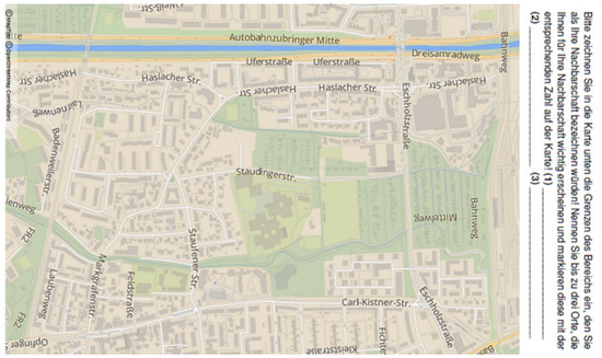
Figure 1.
Illustration of the map as presented on one side of the postcard. ©MapTiler ©OpenStreetMap Contributors.
It is possible that residents living closer to the edges of the shown map are potentially limited in sketching their neighborhood in certain directions. However, we chose the quarter of Haslach-Egerten in particular due to its ‘natural’ boundaries. We thus believe that those residents living closer to the map’s edges were unlikely to extend their self-defined neighborhoods beyond these natural boundaries.
The postcard’s backside consisted of a brief explanation of the study’s purpose, including the information that the postal charges were covered by our department. This was followed by items assessing the participant’s age, gender, and mother tongue. These demographic items were followed by several questions concerning the participant’s living situation, as well as three items assessing their neighborhood relations (see Table 1 for details). The order of all items was fixed. The inclusion of more extensive scales was not possible, due to the limited space on the postcard.

Table 1.
Descriptive information about demographic data and the items assessing neighborhood relations.
2.2.2. Postcard Distribution
The postcards were manually distributed in the study area between October 2019 and January 2020. In each mailbox of each residential building, we dispensed one postcard for every indicated initial or single surname. If only the family name was provided, we dispensed two postcards. We did not dispense postcards for mailboxes belonging to shops, commercials, etc.
Prior to dispensing a postcard, we marked the respective street segment with a UV pen (i.e., leaving a hardly visible marking). In this way, we could trace the approximate location of residence if the postcard was returned, without the need to inquire for the exact address or to violate the participants’ anonymity.
There was no other advertisement for the study and no compensation for participation. Thus, responding to the postcard was entirely voluntary and dependent on the individual resident’s motivation. As a consequence of the chosen approach, we could not specify a sample size in advance; we were limited to the data we received.
2.2.3. Processing of Returned Postcards
Within about three months after the distribution of the last batch of postcards, we received about 450 postcards. Some postcards were returned empty, without any information provided. In several instances, we were unable to locate the UV line marking the participant’s location of residence. More importantly, there was a significant proportion of postcards where participants provided demographic information but did not outline their neighborhood at all, or they did so in undecipherable fashion. Vice versa, there was a small number of postcards with analyzable self-defined neighborhoods; the neighborhoods could not be matched to a statistical district. After identifying the incomplete cases, a final dataset of 277 postcards remained for further analysis. The spatial distribution of these postcards is shown in Figure 2.
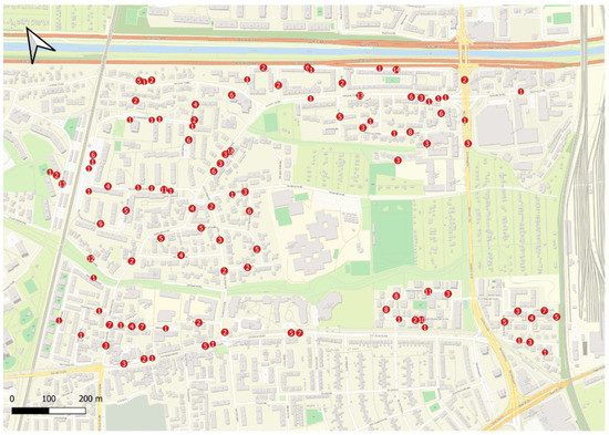
Figure 2.
Spatial distribution of the returned postcards included in the analysis. The approximate location of residence is indicated by red circles, together with the number of postcards from this location.
2.2.4. Demographic Data and Neighborhood Relations
There were postcards from 106 (38.8%) male and 160 (57.8%) female participants (with 11 or 4% missing values). The participants’ average age was 43.9 years (SD = 17.4; range: 8–90; 20% of them 60 years and older). The majority of them indicated German to be their mother tongue (89.9%). Thus, the sample of valid postcards was somewhat biased towards residents of female gender, a younger age, and German nationality as compared to the general population of Haslach-Egerten. Descriptive information about the living situation as well as the level of neighborhood relations reported by the participants is reported in Table 1.
The three items concerning contact, attachment, and trust were thought to assess related, but different aspects of the participants’ relations to their self-defined neighborhoods. A reliability analysis indicated a high internal consistency in the participants’ responses to the three items (Cronbach’s α = 0.89). We thus subsumed them into a combined measure of neighborhood relations (M = 3.6; SD = 1.2; range: 1–5), derived from the mean of all three ratings.
2.2.5. Digitalization and Definition of Neighborhood Boundaries
We aimed to compare links between census-based variables and neighborhood relations based on different neighborhood definitions, namely self-defined, buffer-based, and administrative.
We created a software tool to manually transfer the shape of the self-defined neighborhoods as indicated by the participants to a digital map for further computations and analysis (see Figure 3). We computed the area of each self-defined neighborhood in km2 (M = 0.14 km2; SD = 0.24; range: 0.00–1.20 km2).
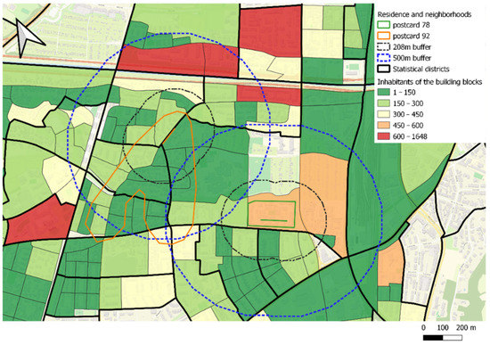
Figure 3.
Illustration of two self-defined neighborhoods, digitalized via our software tool. A line (orange and green, respectively) indicates the approximate home address; the outline of the respective self-defined neighborhood is presented in the same color. The dotted lines in black and blue outline buffers around the home address with a radius of 208 m and 500 m, respectively. Fat black lines outline statistical districts; thin black lines outline building blocks. The colored background indicates the number of inhabitants per building block. ©OpenStreetMap.
We computed two different Euclidian buffers. The first consisted of a 500 m buffer around the line approximating the home address. The second was thought to account for the fact that in our sample, the area of the self-defined neighborhoods consisted of, on average, only a fraction of a 500 m buffer. Based on a circle derived from the average area across all self-defined neighborhoods, we thus computed a second 208 m buffer.
Each postcards’ home address was also linked to one of five statistical districts, as defined by the municipality of Freiburg and thus an instance of an administrative neighborhood definition.
2.2.6. Inclusion of Census-Based Variables
The following variables are based on data provided by the ‘Office of citizen service and information management’ of the municipality of Freiburg. For its own purposes, this office has defined ‘building blocks’ based on a combination of residential blocks, intersecting streets, rail roads, and waters similar to the approach described by [17]. Several demographic data are recorded and updated bi-annually. In accordance with the time of the data collection, we used the respective dataset valid for the first half of 2019.
For the purpose of this research, we extracted the following variables for each building block:
- Proportion of German residents: The number of residents with a German nationality divided by the total number of residents.
- Average number of people per household: The dataset provided information about the number of people per household in the following categories: 1 person; 2 persons; 3 persons; 4 persons; 5 persons and more persons. As an approximation of the average household size in a given neighborhood, we multiplied the value of each category (i.e., 1 for one person, 2 for two persons, etc.) with the respective number of residents in this category and divided the sum of these multiplications by the total number of residents in this building block. This variable also reflects the proportion of families with children.
- Average number of homes per building: The dataset provided information about the number of homes per building in the following categories: 1–2 homes; 3–5 homes; 6–7 homes; 8–9 homes; 10 and more homes. Corresponding to the method described above, we computed an estimate of the average number of homes per building by multiplying the lowest value of each category (e.g., 3 for the category ‘3–5 homes’) with the respective number of residents in this category, relative to the total number of residents in this building block. Using the lowest value of each category underestimates the true number of homes per building and should thus be treated as a rough estimate rather than a precise measure. However, this was the most consistent approach we could think of.
- Proportion of seniors: The dataset provided only very rough information about the residents’ age. The most relevant and clearly identifiable variable was the number of elderly people (60+ years). We computed the proportion of seniors by dividing the number of residents aged 60 years and older by the total number of residents.
Unfortunately, the office of citizen service and information management was unable to provide sufficiently granular information concerning some variables that have previously been investigated, for example, the unemployment rates or crime rates, e.g., [11,12,14,22]. (Please note that, for example, unemployment rates are available for the entire quarter of Haslach. However, this information is too coarse to be linked to the neighborhood concepts investigated in this research.)
Next, we linked the census data of the building blocks to the four different neighborhood boundaries. For each participant, we computed the proportion of each building block located within the respective neighborhood boundary and combined the census variables according to the proportions of all involved building blocks. (If, for example, a self-defined neighborhood consisted of 50% of one building block with 10% seniors and 50% of a second building block with 30% seniors, this would result in 20% seniors for the entire self-defined neighborhood. If the 208 m buffer of the same participant would consist of 25% of the building block with 10% seniors and 75% of the second building block with 30% seniors, this would result in 25% seniors for the entire neighborhood based on a 208 m buffer.) Descriptive census-based variables, separately for all four neighborhood boundaries, are presented in Table 2.
Table 2.
Information concerning the census-based variables, separately for all four neighborhood boundaries. The first block presents their descriptive statistics (M (SD; range)). The second block presents the proportional overlap of the self-defined neighborhoods with the other three neighborhood definitions (M (SD; range)). The third block presents the Pearson correlation coefficient of the self-defined neighborhoods with the other three neighborhood definitions, separately for all four census-based variables (** = p < 0.01, *** = p < 0.001).
3. Results
3.1. Neighborhood Size and Shape
In a first step, we took a closer look at the shape and size of the self-defined neighborhoods. The area defined as neighborhood (M = 0.14 km2; SD = 0.24; range: 0.00–1.20 km2) was on average about as large as four of the five statistical districts (0.11–0.16 km2, with the fifth district covering 0.58 km2) and comparable to that of the 208 m buffer (M = 0.19 km2; SD = 0.02; range: 0.14–0.24 km2), but much smaller as compared to the area of a 500 m buffer (M = 0.91 km2; SD = 0.06; range: 0.80–1.06 km2. The variance in size of the buffer-based neighborhood areas resulted from the different length of the street segments we identified as the residents’ home address). The overlap of the self-defined neighborhoods with the statistical districts and especially with the 500 m buffer was rather limited (see Table 2). However, even after accounting for the average area of the self-defined neighborhoods, the overlap of the resulting 208 m buffer with the self-defined neighborhoods remained poor.
It could be argued that the limited overlap does not matter, because the census-based variables presented in Table 2 do not appear to vary greatly between the different neighborhood definitions. However, when we computed Pearson correlations between the census variables adjusted to the self-defined neighborhoods and the same census variables adjusted to the other three neighborhood definitions, respectively, we found very heterogeneous correlation coefficients, ranging from very high fits to no fit at all. The average number of people per household was the only census variable showing consistently high (although still far from perfect) correlations.
Taken together, and in line with previous findings, e.g., [1,3,18,19,20], it is safe to say that neither administrative definitions of neighborhood nor fixed Euclidian buffers are representative for the area residents themselves define as their neighborhood.
This begs the question of which factors affect and determine the size and shape of self-defined neighborhoods. Detailed investigations of the neighborhoods’ shape were beyond the scope of this research. However, we decided to take a closer look at the size of the self-defined neighborhoods (i.e., their area). Previous studies already showed that demographic variables affect the area an individual resident defines as neighborhood [4,16]. Adding the census-based variables to such an analysis should provide first evidence whether variables derived from census data have an effect on residents’ conceptions of their neighborhood on a physical level. Thus, we constructed a linear mixed model with the area of the self-defined neighborhoods as the dependent variable (Model 1). Independent variables of this model are as follows:
- Neighborhood relations. The compound measure consisting of the self-reported levels of contact, attachment, and trust.
- Demographics and self-reported living situation. Gender and mother tongue were treated as categorical factors. The number of children was turned into a categorical variable (no children vs. one or more children) due to the odd distribution, with 69.7% of the participants stating that no minors lived at their household. All other variables were treated as continuous factors.
- Census-based variables, as reported in the previous section, and adjusted to the area of the self-defined neighborhood of each participant.
All statistical details concerning Model 1 are presented in Table 3. (Please note that 15 cases were not included in Model 1, Model 5, and Model 6 due to missing values for single variables.) In line with Coulton and colleagues [16], the self-defined neighborhoods grew smaller with the resident’s age. Contrasting Coulton and colleagues [16], we found no evidence that the participants’ gender, children in the household, or the years of residency had an impact on the neighborhood area. However, residents reporting to live in larger households defined smaller areas as their neighborhood. The model shows no significant evidence of a link between neighborhood relations and the area of the self-defined neighborhood. More importantly, there were several significant effects linked to the census-based variables: a higher proportion of German residents and a higher average number of people per household resulted in smaller self-defined neighborhoods. A higher proportion of senior citizens increased the area defined as neighborhood. In other words, Model 1 provided strong evidence that attributes of the surrounding urban environment as captured by census-based variables have an effect on how residents define their neighborhood.
Table 3.
Parameter estimates of the linear mixed model testing links between demographic factors and census-based variables to the area defined as neighborhood (Model 1). * = p < 0.05, ** = p < 0.01.
3.2. Neighborhood Relations
We now turn towards the question to what extent different conceptualizations of ‘neighborhood’ can predict neighborhood relations. For this purpose, we constructed four linear mixed models with neighborhood relations as the dependent variable, and the four census-based variables as independent variables. In Model 2, the census-based variables were linked to a resident’s statistical district. In Model 3, the census-based variables were defined by a 500 m buffer around a resident’s home address. The census-based variables of Model 4 reflected a 208 m buffer. In Model 5, the census-based variables were linked to the self-defined neighborhoods. All statistical details for these models are presented in Table 4.
Table 4.
Parameter estimates of the linear mixed models testing links between neighborhood relations and census-based variables derived from four different neighborhood boundary definitions. * = p < 0.05, ** = p < 0.01, *** = p < 0.001.
The results of Models 2–5 are in line with our hypotheses. Census-based variables based on administrative units failed to predict neighborhood relations (Model 2). When based on a 500 m buffer (Model 3), we found that both a higher proportion of Germans and a larger number of people per household increased neighborhood relations. We found corresponding effects when adjusting the buffer to a radius of 208 m in Model 4, with an additional effect indicating a lower number of homes per building benefiting neighborhood relations. Finally, when we predicted neighborhood relations from census variables based on the actual self-defined variables in Model 5, we observed strong effects for both the number of people per household and the number of households per building. Additionally, there was a somewhat curious and positive effect for the proportion of seniors. Contrasting Models 3 and 4, there was no effect for the proportion of Germans. The comparison of the parameter estimates already suggests that the prediction of neighborhood relations increases with a better approximation of the residents’ neighborhood. This interpretation is further strengthened by the model fit—whereas Nagelkerke’s Pseudo-R2 was about comparable for Models 2–4, it was noticeable increased in Model 5.
It could be argued that the identified links between census-based variables and neighborhood relations are of little use. If we need to collect data (i.e., the self-defined neighborhood) from the individual citizen for a more precise prediction of neighborhood relations, we may as well collect information demographics and self-reported living conditions as more established indicators of neighborhood relations. Thus, the question is whether local urban characteristics as captured in census-based variables can provide insights into neighborhood relations beyond demographic factors and self-reported living conditions.
We addressed this issue by testing the effects of demographic variables and self-reported living conditions on neighborhood relations with Model 6. As can be derived from Table 5, we found better neighborhood relations for women as compared to men, for residents with children as compared to those without, and for those reporting German to be their mother tongue, also see [11,14]. Furthermore, neighborhood involvement increased with the residents’ age. Taken together, Model 6 shows a very plausible pattern concerning the effects of demographic factors but less evidence for effects of self-reported living conditions on neighborhood relations.
Table 5.
Parameter estimates of two linear models testing links between neighborhood relations and demographic factors (Model 6), as well as demographic factors and census-based variables (Model 7). * = p < 0.05, ** = p < 0.01, *** = p < 0.001.
Next, we ran Model 7, which included the census-based variables (adjusted to the self-defined neighborhood, thus corresponding to the data used in Model 5) in addition to the demographic factors tested in Model 6. There were slight changes concerning the effects of demographic variables. The difference between residents with children and those without missed significance (p = 0.06). However, the combined model indicates a positive effect of the years of residency on neighborhood relations, which we did not observe in Model 6. The parameter estimates of the census-based variables resemble those of Model 5, with a significant positive effect of the average number of people per household, and a negative effect of the homes per building just missing significance (p = 0.06). However, the effect resulting from the proportion of seniors observed in Model 5 did not appear in Model 7. More importantly, a model comparison indicated that the addition of census-based variables in Model 7 predicted neighborhood relations significantly better than demographic variables alone (as is also evident from the increase of Nagelkerke’s Pseudo-R2).
4. Discussion
In the present research, we collected a dataset of self-defined neighborhoods, together with self-reports on demographic factors, living-conditions, and neighborhood relations (derived from three items assessing the level of contact with and trust in neighbors, as well as the attachment to the residential neighborhood). We aimed at contrasting the self-defined neighborhoods with three different neighborhoods defined by the statistical district, and a 500 m buffer as well as a 208 m buffer, each depending on the resident’s home address. Furthermore, we linked several census-based variables (e.g., the proportion of seniors or the average household size) to the different neighborhood definitions.
We found that the area of the self-defined neighborhoods covered only a fraction of the frequently assumed neighborhood definitions defined by administrative units or fixed buffers of 500 m or more. The spatial overlap of the area based on the different boundaries with the area of the self-defined neighborhoods was on average very limited in line with, for example, [20,21]. In other words, our findings provide strong evidence that one-size-fits-all approaches are not sufficient to capture the individual resident’s neighborhood definitions. In line with Coulton and colleagues [16], we found that the area defined as neighborhood was affected by demographic factors. More importantly, we also observed strong effects of census-based variables. These effects underline that the structure and attributes of the urban environment affect residents’ perceptions of their neighborhood.
After adjusting several census-based variables to the shape and size of the different neighborhood definitions, we aimed at predicting the residents’ neighborhood relations from these variables. In short, we found that census-based variables allow for a better prediction of neighborhood relations, the closer the census-based variables are adjusted to the neighborhood definition of the individual resident. Furthermore, census-based variables explained variance of neighborhood relations in addition to the residents’ demographic factors and self-reported living conditions.
Taken together, our findings underline the importance of adjusting the concepts of ‘neighborhood’ underlying one’s research to those of the residents under investigation, in particular when studying neighborhood attachment or sense of community but also see [29], for a different approach based on social networks. The pattern of the different neighborhood definitions suggests that assuming a more-narrow area as neighborhood than frequently assumed (e.g., buffers of 500 m or 1 mile) allows better predictions of neighborhood relations from census-based variables.
4.1. Limitations
Our postcard-based approach for the data collection allowed for only a minimum of items. Thus, we were not able to rely on established and more extensive questionnaires assessing neighborhood attachment or sense of community (see [6], for an overview). However, our findings on demographic factors are very much in line with those reported by previous research [12,14], and we are thus confident that we successfully tapped into concepts closely related to the participants’ neighborhood attachment.
A further restriction was imposed by the fixed area and scale of the map printed on the postcards. It is possible that some participants were biased when defining their neighborhood. However, the great variability of the areas and shapes of the self-defined neighborhoods imply that the vast majority of the participants was not limited by the presented format. Most of the self-defined neighborhoods also covered only a fraction of the postcard. Finally, we deliberately chose Haslach-Egerten because we assumed that railroads and a river provided strong ‘natural’ boundaries for those residents living closer to the edges of the map shown on the postcard.
Participation in the study was voluntarily, and we cannot exclude potential biases elicited by socio-demographic groups that were more (or less) inclined to return the postcard. The demographic distribution of residents returning valid postcards was somewhat skewed (with a higher proportion of female and younger participants, as well as a higher proportion of residents with a German nationality) but not entirely off-balanced when compared to the general population of Haslach-Egerten. Although it is possible that the self-defined neighborhoods of potentially under-represented socio-demographic groups differ from those we invested, we do not believe that this invalidates our main conclusion. We cannot think of a reason why administrative units or buffer-based neighborhood definitions should be more appropriate for these groups as compared to those who participated in the study.
Unfortunately, we were unable to obtain census data concerning some variables that have previously been investigated and identified as important for neighborhood relations in the necessary spatial resolution, for example, unemployment and crime rates, e.g., [11,12,14,22]. We assume that the general pattern of a closer adjustment to the self-defined neighborhood allowing a better prediction of neighborhood relations from census-based variables extends to these variables as well.
4.2. Towards Identifying Individual and Shared Neighborhood Cores and Boundaries
We assume that although residents’ self-defined neighborhoods living in the same area are highly individual, that they are also are affected by the same parameters, and that their neighborhood concepts should thus show some level of convergence. Next to census-based variables, these parameters may encompass demographic factors [30,31]; the accessibility of urban resources and institutions [1,31]; and physical cues such as roads, large building complexes, or waters, e.g., [30,32]. Indeed, several attempts of aggregating across self-defined neighborhoods imply the existence of neighborhood boundaries and cores mutually shared by the majority of the local residents [28,30,31,33,34,35]. These findings support the idea of using participatory GIS approaches in community-based planning and neighborhood revitalization programs [26,27], as well as with the assumption of a ‘spatial collective intelligence’ [36].
Finally, we want to point out the long and intensive occupation of social epidemiologists and sociologists with the effects of neighborhoods on their residents [5]. A more detailed depiction of the discussions and findings from this field are far beyond this research. Despite differences in focus and methodology, it appears that there are some conclusions converging to our research: administrative borders do not reflect the communities that develop within and across them [23]. Establishing the spatial links between individual residents and their shared community may also support attempts to understand the effects of neighborhood on their residents.
5. Conclusions
In line with previous research, we found that both administrative units and buffer-based neighborhood definitions show limited overlap with the area defined by the residents themselves. This limited overlap explains why several studies failed to find links between residents’ subjective neighborhood relations (e.g., trust or attachment) and census-based variables (i.e., objective indicators about living conditions and the surrounding environment). Our findings emphasize that living conditions assessed via census-based variables are more informative about residents’ subjective neighborhood relations when they are closer adjusted to the neighborhood definition of the individual resident. If we better understand the factors determining the boundaries of the area a resident feels attached to and cares for, initiatives to increase neighborly interactions and efforts in this area are more likely to be successful. Furthermore, urban planners and policy makers can use this knowledge to shape or alter the residents’ engagement in their neighborhood [7,8].
Author Contributions
Conceptualization, R.v.S.; Methodology, R.v.S.; Software, D.B. and F.F.; Formal Analysis, R.v.S.; Data Curation, D.B. and F.F.; Writing—Original Draft Preparation, R.v.S.; Writing—Review & Editing, D.B. and F.F.; Visualization, D.B. and F.F.; Supervision, R.v.S.; Funding Acquisition, R.v.S. All authors have read and agreed to the published version of the manuscript.
Funding
This research was supported by a grant of the German BMBF to the first author (Grant number 16SV7405). The article processing charge was funded by the Open Access Publication Fund of the University of Freiburg.
Institutional Review Board Statement
The study was conducted in accordance with the Declaration of Helsinki. Ethical review and approval were waived for this study, because participants were not deceived and there was no foreseeable harm resulting from participation.
Informed Consent Statement
On the bottom of the postcard’s backside (see Section 2.2), it was clarified that participation was voluntarily, and that by returning the postcard, participants gave their consent to an anonymized processing and analysis of their data. Additional information and contact details were provided on a website, which was indicated on the postcard as well.
Data Availability Statement
Data are available on request to the first author.
Acknowledgments
We thank Svenja Dehner and Leonie Holdik for their help with the distribution and digitalization of the postcards. We thank the Office of Citizen Service and Information Management of the city of Freiburg for providing us with the census data. We thank two anonymous reviewers for their valuable input.
Conflicts of Interest
The authors declare no conflict of interest.
References
- Vallée, J.; Le Roux, G.; Chaix, B.; Kestens, Y.; Chauvin, P. The ‘Constant Size Neighbourhood Trap’ in Accessibility and Health Studies. Urban. Stud. 2015, 52, 338–357. [Google Scholar] [CrossRef]
- Bernardo, F.; Palma-Oliveira, J.-M. Urban Neighbourhoods and Intergroup Relations: The Importance of Place Identity. J. Environ. Psychol. 2016, 45, 239–251. [Google Scholar] [CrossRef]
- Charreire, H.; Feuillet, T.; Roda, C.; Mackenbach, J.D.; Compernolle, S.; Glonti, K.; Bárdos, H.; Le Vaillant, M.; Rutter, H.; McKee, M.; et al. Self-Defined Residential Neighbourhoods: Size Variations and Correlates across Five European Urban Regions. Obes. Rev. 2016, 17, 9–18. [Google Scholar] [CrossRef] [PubMed] [Green Version]
- Colabianchi, N.; Coulton, C.J.; Hibbert, J.D.; McClure, S.M.; Ievers-Landis, C.E.; Davis, E.M. Adolescent Self-Defined Neighborhoods and Activity Spaces: Spatial Overlap and Relations to Physical Activity and Obesity. Health Place 2014, 27, 22–29. [Google Scholar] [CrossRef] [PubMed] [Green Version]
- Oakes, J.M.; Andrade, K.E.; Biyoow, I.M.; Cowan, L.T. Twenty Years of Neighborhood Effect Research: An Assessment. Curr. Epidemiol. Rep. 2015, 2, 80–87. [Google Scholar] [CrossRef] [Green Version]
- Lewicka, M. Place Attachment: How Far Have We Come in the Last 40 Years? J. Environ. Psychol. 2011, 31, 207–230. [Google Scholar] [CrossRef]
- Brown, B.; Perkins, D.D.; Brown, G. Place Attachment in a Revitalizing Neighborhood: Individual and Block Levels of Analysis. J. Environ. Psychol. 2003, 23, 259–271. [Google Scholar] [CrossRef]
- Dang, L.; Seemann, A.-K.; Lindenmeier, J.; Saliterer, I. Explaining Civic Engagement: The Role of Neighborhood Ties, Place Attachment, and Civic Responsibility. J. Community Psychol. 2021. [Google Scholar] [CrossRef]
- Scannell, L.; Gifford, R. The Experienced Psychological Benefits of Place Attachment. J. Environ. Psychol. 2017, 51, 256–269. [Google Scholar] [CrossRef]
- Jenks, M.; Dempsey, N. Defining the Neighbourhood: Challenges for Empirical Research. Town Plan. Rev. 2007, 78, 153–177. [Google Scholar] [CrossRef]
- French, S.; Wood, L.; Foster, S.A.; Giles-Corti, B.; Frank, L.; Learnihan, V. Sense of Community and Its Association With the Neighborhood Built Environment. Environ. Behav. 2014, 46, 677–697. [Google Scholar] [CrossRef]
- Lee, S.M.; Conway, T.L.; Frank, L.D.; Saelens, B.E.; Cain, K.L.; Sallis, J.F. The Relation of Perceived and Objective Environment Attributes to Neighborhood Satisfaction. Environ. Behav. 2017, 49, 136–160. [Google Scholar] [CrossRef]
- Bonaiuto, M.; Fornara, F.; Bonnes, M. Indexes of Perceived Residential Environment Quality and Neighbourhood Attachment in Urban Environments: A Confirmation Study on the City of Rome. Landsc. Urban. Plan. 2003, 65, 41–52. [Google Scholar] [CrossRef]
- Zahnow, R.; Tsai, A. Crime Victimization, Place Attachment, and the Moderating Role of Neighborhood Social Ties and Neighboring Behavior. Environ. Behav. 2019, 0013916519875175. [Google Scholar] [CrossRef]
- De Marco, A.; De Marco, M. Conceptualization and Measurement of the Neighborhood in Rural Settings: A Systematic Review of the Literature. J. Community Psychol. 2010, 38, 99–114. [Google Scholar] [CrossRef]
- Coulton, C.J.; Jennings, M.Z.; Chan, T. How Big Is My Neighborhood? Individual and Contextual Effects on Perceptions of Neighborhood Scale. Am. J. Community Psychol. 2013, 51, 140–150. [Google Scholar] [CrossRef]
- Cutchin, M.P.; Eschbach, K.; Mair, C.A.; Ju, H.; Goodwin, J.S. The Socio-Spatial Neighborhood Estimation Method: An Approach to Operationalizing the Neighborhood Concept. Health Place 2011, 17, 1113–1121. [Google Scholar] [CrossRef] [Green Version]
- Siordia, C.; Coulton, C.J. Using Hand-Draw Maps of Residential Neighbourhood to Compute Level of Circularity and Investigate Its Predictors. Hum. Geogr.— J. Stud. Res. Hum. Geogr. 2015, 9, 131–149. [Google Scholar] [CrossRef]
- von Stülpnagel, R.; Brand, D.; Seemann, A.-K. Your Neighbourhood Is Not a Circle, and You Are Not Its Centre. J. Environ. Psychol. 2019, 66, 101349. [Google Scholar] [CrossRef]
- Bödeker, M. Walking and Walkability in Pre-Set and Self-Defined Neighborhoods: A Mental Mapping Study in Older Adults. Int. J. Environ. Res. Public. Health 2018, 15, 1363. [Google Scholar] [CrossRef] [Green Version]
- Smith, G.; Gidlow, C.; Davey, R.; Foster, C. What Is My Walking Neighbourhood? A Pilot Study of English Adults’ Definitions of Their Local Walking Neighbourhoods. Int. J. Behav. Nutr. Phys. Act. 2010, 7, 8. [Google Scholar] [CrossRef] [PubMed] [Green Version]
- Grogan-Kaylor, A.; Woolley, M.; Mowbray(deceased), C.; Reischl, T.M.; Gilster, M.; Karb, R.; Macfarlane, P.; Gant, L.; Alaimo, K. Predictors of Neighborhood Satisfaction. J. Community Pract. 2006, 14, 27–50. [Google Scholar] [CrossRef]
- Krase, J. Seeing Community in a Multicultural Society: Theory and Practice. In Perspectives of Multiculturalism: Western and Transitional Countries; Croatian Commission for UNESCO; FF Press: Zagreb, Croatia, 2004; pp. 151–177. [Google Scholar]
- Dunn, C.E. Participatory GIS—A People’s GIS? Prog. Hum. Geogr. 2007, 31, 616–637. [Google Scholar] [CrossRef]
- Flanagin, A.J.; Metzger, M.J. The Credibility of Volunteered Geographic Information. GeoJournal 2008, 72, 137–148. [Google Scholar] [CrossRef]
- Mukherjee, F. Public Participatory GIS. Geogr. Compass 2015, 9, 384–394. [Google Scholar] [CrossRef]
- Elwood, S.; Leitner, H. GIS and Spatial Knowledge Production for Neighborhood Revitalization: Negotiating State Priorities and Neighborhood Visions. J. Urban. Aff. 2003, 25, 139–157. [Google Scholar] [CrossRef]
- Dalton, N. Is Neighbourhood Measurable. In Proceedings of the 6th International Space Syntax Symposium, Istanbul, Turkey, 12–15 June 2007; Volume 88, pp. 1–12. [Google Scholar]
- Hipp, J.R.; Faris, R.W.; Boessen, A. Measuring ‘Neighborhood’: Constructing Network Neighborhoods. Soc. Netw. 2012, 34, 128–140. [Google Scholar] [CrossRef] [Green Version]
- Campbell, E.; Henly, J.R.; Elliott, D.S.; Irwin, K. Subjective Constructions of Neighborhood Boundaries: Lessons from a Qualitative Study of Four Neighborhoods. J. Urban. Aff. 2009, 31, 461–490. [Google Scholar] [CrossRef]
- van Gent, W.P.C.; Boterman, W.R.; van Grondelle, M.W. Surveying the Fault Lines in Social Tectonics; Neighbourhood Boundaries in a Socially-Mixed Renewal Area. Hous. Theory Soc. 2016, 33, 247–267. [Google Scholar] [CrossRef] [Green Version]
- Kramer, R. Defensible Spaces in Philadelphia: Exploring Neighborhood Boundaries Through Spatial Analysis. RSF Russell Sage Found. J. Soc. Sci. 2017, 3, 81–101. [Google Scholar] [CrossRef]
- Goldblatt, R.; Omer, I. “Perceived Neighbourhood” and Tolerance Relations: The Case of Arabs and Jews in Jaffa, Israel. Local Environ. 2016, 21, 555–572. [Google Scholar] [CrossRef]
- Bae, C.; Montello, D. Representations of an Urban Ethnic Neighbourhood: Residents’ Cognitive Boundaries of Koreatown, Los Angeles. Built Environ. 2018, 44, 218–240. [Google Scholar] [CrossRef]
- Phillips, D.W.; Montello, D.R. Defining the Community of Interest as Thematic and Cognitive Regions. Polit. Geogr. 2017, 61, 31–45. [Google Scholar] [CrossRef]
- Spielman, S.E. Spatial Collective Intelligence? Credibility, Accuracy, and Volunteered Geographic Information. Cartogr. Geogr. Inf. Sci. 2014, 41, 115–124. [Google Scholar] [CrossRef] [PubMed]
Publisher’s Note: MDPI stays neutral with regard to jurisdictional claims in published maps and institutional affiliations. |
© 2022 by the authors. Licensee MDPI, Basel, Switzerland. This article is an open access article distributed under the terms and conditions of the Creative Commons Attribution (CC BY) license (https://creativecommons.org/licenses/by/4.0/).