Prediction of the Stability of Various Tunnel Shapes Based on Hoek–Brown Failure Criterion Using Artificial Neural Network (ANN)

Abstract

In this paper, artificial neural network (ANN) models are presented in order to enable a prompt assessment of the stability factor of tunnels in rock masses based on the Hoek–Brown (HB) failure criterion. Importantly, the safety assessment is one of the serious concerns for constructing tunnels and requires a reliable and accurate stability analysis. However, it is challenging for engineers to construct finite element limit analysis (FELA) algorithms with the HB failure criterion for tunnel stability solutions in rock masses. For the first time, a machine-learning-aided prediction of tunnel stability based on the HB failure criterion is proposed in this paper. Three different shapes of tunnels, i.e., heading tunnel, dual square tunnels, and dual circular tunnels, are considered. The inputs include four dimensionless parameters for the heading tunnel including the cover-depth ratio, the normalized uniaxial compressive strength, the geological strength index (GSI), and the m_i parameter. Moreover, dual square and circular tunnels include one more additional parameter namely the distance ratio. The results present the best ANN models for each tunnel shape, providing very reliable solutions for predicting the tunnel stability based on the HB failure criterion.

1. Introduction

A tunnel in a rock mass is commonly constructed using the bored tunnel technique. There are conventional and mechanized methods that can be utilized in the construction depending on the dimensions of the tunnel and the characteristics of the rock mass. One of the conventional methods is to use blasting techniques for tunnel constructions in hard rock formations, where the issue of support is usually minor. On the other hand, tunnels may be constructed in weak rock formations by using mechanical excavators, in which case, heavy supports, such as shotcrete, anchors/bolts, and steel ribs, are required during the construction. In addition to the blasting and drilling methods, a tunnel boring machine (TBM) is an efficient technique for tunnel construction in rock masses. This TBM method can also be designed to excavate noncircular tunnels such as tunnels with square shapes. Commonly, an open-type TBM is used for tunnel construction in hard rock. For fractured rocks and highly broken rocks, a single-shield or double-shield TBM is widely utilized to ensure the safety of rock masses while constructing. To precisely evaluate the tunnel stability in rocks during tunnel construction, an effective failure criterion for capturing rock collapse is necessary.

The Hoek–Brown (HB) failure criterion was first created analytically in the 1980s by curve-fitting triaxial test data of whole and jointed rocks and is known as the original HB criterion 1980 (Hoek and Brown [1]). Hoek et al. [2] performed changes to the original version in an attempt to optimize the effect of the highly fractured property. This version from 2002 has now become the most famous HB failure criterion. Hoek gives a quick overview of the failure criteria’s origins and progress [3,4]. The HB failure criterion has a more intricate nonlinear expression than the linear Mohr–Coulomb failure criterion, most notably the reliance of rock mass shear strength on the nonlinearity of the minor principal compressive stress. In order to appropriately reflect the failure of jointed rock masses, the HB failure criteria require extra strength factors.

Although this HB failure criterion may be employed to correctly define the failure characteristics of diverse rock types, it has been used to examine multiple challenges in the area of rock engineering, such as subterranean entrances and caves (e.g., Carranza-Torres and Fairhurst [5]; Carranza-Torres [6]; Fraldi and Guarracino [7]; Martin et al. [8]; Sakurai [9]; Senent et al. [10]; Swift and Reddish [11]; Yang and Huang [12]; [13]), bearing capacity and shaft resistance of foundations (e.g., AlKhafaji et al. [14]; Chakraborty and Kumar [15]; Clausen [16]; Keshavarz and Kumarm [17]; Merifield, et al. [18]; Saada et al. [19]; Serrano and Olalla [20]; [21]; Yodsomjai et al. [22]; Keawsawasvong [23]; Keawsawasvong et al. [24]; [25]; Yang and Yin [26]), and stability analysis of rock slopes (Yodsomjai et al. [27]; Deng et al. [28]; Li et al. [29]; [30]; Shen and Karakus, [31]; Shen et al. [32]; Yang et al. [33]; You et al. [34]).

The finite element limit analysis (FELA) technique developed by Sloan [35] is a strong tool for obtaining the required stability results. Plastic bounds theorems, finite element discretization, and nonlinear programming are all applied in this method. Following a completely plastic material with an associated flow rule, the relevant upper and lower bound theorems (UB and LB) are established. An exact solution should be able to be bracketed from both above (UB) and below (LB). The HB model was combined with the FELA (Kumar and Rahaman [36]) to produce tunnel stability solutions to analyze the stability of unlined tunnels in rock masses. As a result, a number of prior studies have lately focused on tunnel stability in HB rock masses with different shapes. Keawsawasvong and Ukritchon [37] investigated the stability of a single circular tunnel, whereas Ukritchon and Keawsawasvong [38] and Xiao et al. [39] investigated the stability of a single square tunnel and a single rectangular tunnel, respectively. Ukritchon and Keawsawasvong [40] have explored the rock stability solutions for plane strain heading tunnels. Furthermore, Zhang et al. [41] and Xiao et al. [42] evaluated the stability of dual unlined circular and square tunnels, respectively.

The aforementioned studies relate to the use of FELA with the HB failure criterion to investigate the stability of tunnels that are located in rock masses. However, soft computing emerged as a viable alternative to the traditional analytic and numerical methodologies. An artificial neural network is a form of soft computing technology (ANN). This method can acquire from a large enough dataset employed to generate a black-box prediction model to utilize the results in the form of a closed simple equation. The ANN approach has been used to determine rock properties in the field of rock engineering (e.g., Gholami et al. [43]; Mert et al. [44]; Miah et al. [45]; Mohamad Ali Ridho et al. [46]; Ocak and Seker [47]; Yang and Zhang [48]; Keawsawaswong et al. [49]). Alavi and Sadrossadat [50], Millán et al. [51], and Ziaee et al. [52] applied the ANN approach to develop models for forecasting the consequences of problems with foundation bearing capacity on rock masses. Li et al. [53] utilized the dataset acquired from FELA with the HB failure criterion to suggest the scheme for predicting stability solutions of rock slopes using an extreme learning neural network and a terminal steepest descent method. Recently, Naghadehi et al. [54] have used the ANN approach to investigate the face stability of mechanized shield tunneling in cohesive-frictional soils. However, no prior research has used the ANN approach to examine the stability of tunnels in rock masses using FELA with the HB failure criterion. This research created a practical tool based on the ANN approach that can quickly evaluate tunnel stability for varied designs.

2. Problem Definition and Hoek–Brown Failure Criterion

The Hoek–Brown (HB) failure criteria (Hoek and Brown [1]; Hoek et al. [2]) is a well-known rock failure model that accounts for the minor principal (compressive) stress’s nonlinearity. The HB failure criterion is expressed mathematically as a power-law relationship between the major and minor principal stresses (i.e., σ₁ and σ₃). Considering tensile normal stresses as a positive parameter, the HB failure criterion is as follows:

$$\hspace{0.17em}{\sigma }_3={\sigma }_1-{\left(-m_b{\sigma }_1{(-{\sigma }_{ci})}^{(1-a)/a}+s{(-{\sigma }_{ci})}^{1/a}\right)}^a$$

(1)

where σ_ci is the uniaxial compressive strength of intact rock mass while m_b, s, and a are expressed in Equations (2)–(4).

$$a=\frac{1}{2}\hspace{0.17em}+\frac{1}{6}\left\{\exp \left(\frac{-GSI}{15}\right)-\exp \left(\frac{-20}{3}\right)\right\}$$

(2)

$$m_b=\hspace{0.17em}{m}_i\exp \left(\frac{GSI-100}{28-14DF}\right)$$

(3)

$$s=\hspace{0.17em}\exp \left(\frac{GSI-100}{9-3DF}\right)$$

(4)

The geological strength index (GSI) usually ranges from 10 to 100 (from a heavily damaged rock mass to a completely undamaged rock mass). The degree of disturbance is denoted by DF, which normally runs between 0 and 1 (in situ rock masses that have not been disturbed to in situ rock masses that have been severely disrupted). The value of m_i is normally between 5 and 35. This is a constant that is proportional to the frictional strength of an entire rock mass.

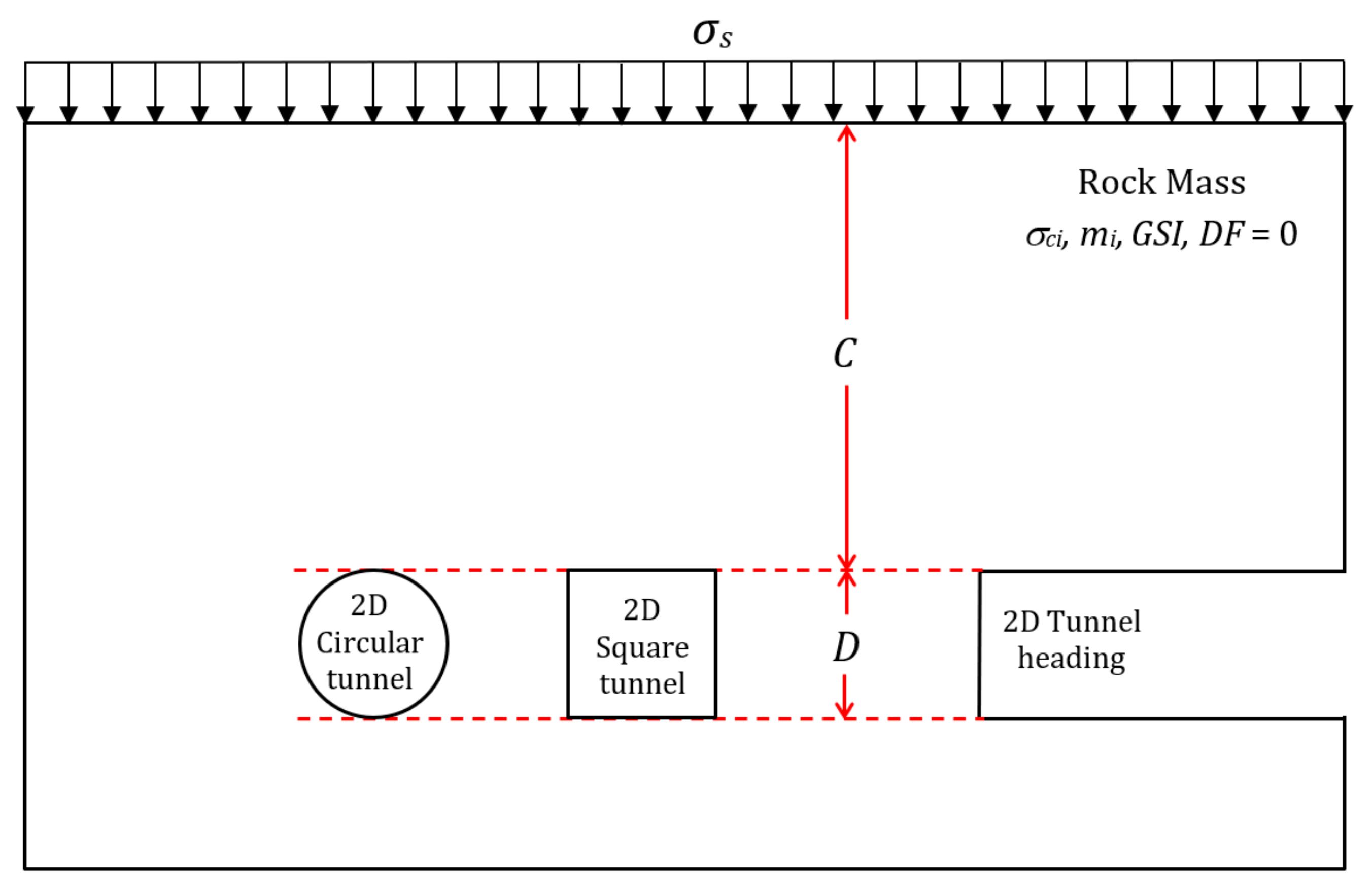
Figure 1 shows three different 2D unlined tunnels under a plane strain condition, namely the circular, the square, and the tunnel heading. In this study, since a plane strain condition is assumed, the assumption for the circular and the square tunnels is that the problem represents a very long unlined tunnel. The 2D tunnel heading problem is treated as a longwall mining problem with an infinitely long flat wall. The tunnels have a diameter (D) and a cover depth (C) above the crown. The rock mass has a unit weight of γ, and at the surface area of rock masses, a uniform surcharge pressure at collapse (σ_s) is applied over the area. It is hypothesized that there is no disturbance in the surrounding rock mass during tunnel excavation and the undisturbed in situ condition is applicable to the HB model with the disturbance factor DF = 0. For the problem of dual unlined circular and square tunnels, the center-to-center distance between the tunnels is defined as S, as shown in Figure 2.

According to the above-mentioned parameters, seven design parameters were considered in this study (i.e., C, D, S, σ_ci, GSI, m_i, γ). Using the dimensionless output parameter (σ_s/σ_ci), where σ_s is the uniform surcharge at collapse. Equation (5) represents the stability factor (σ_s/σ_ci) as a function of five dimensionless parameters.

$$\frac{{\sigma }_s}{{\sigma }_{ci}}=f(\frac{C}{D},\frac{\gamma D}{{\sigma }_{ci}},m_i,GSI,\frac{S}{D})$$

(5)

where S/D is the distance ratio; C/D is the cover-depth ratio; γD/σ_ci is the normalized unit weight ratio; GSI is the geological strength index; m_i is the frictional strength of intact rock; and σ_s/σ_ci is the stability factor. It should be noted that, for the tunnel heading problem, the distance ratio S/D was not taken into account. It is noted that the training datasets were collected from the FELA solutions derived from previously published works. The aim of this study is to develop a nonlinear input–output mapping employing an extreme machine learning approach to develop a neural network model for a system of tunnels in rock masses.

3. Method

3.1. Artificial Neural Network (ANN)

An artificial neural network (ANN) is a data prediction framework that is based on pre-existing elements taken from the human mind’s structure. When dealing with intricate information, it simulates the nervous system’s processing technique in the human brain. The applications of the ANN have been proved to be a very efficient soft-computing approach in the civil engineering field [55,56,57,58,59,60,61,62,63,64]. A neural network is a computer model made up of many interconnected nodes (or neurons). This network is made up of neurons that are in the form of functional blocks. Weights are used to link neurons, which are typically chosen randomly at the beginning. As the learning process progresses, the weights in the network are gradually raised or lowered until they reach the required level that can be used to predict the target with reasonable accuracy (Park and Lek [65]). This method is particularly well suited for addressing nonlinear problems.

As shown in Figure 3, the required output may be achieved in a trained neural network by accepting inputs while taking into consideration the updated weights. The network improves over time by comparing the intended input and output and identifying the mistake. The accuracy of the prediction model and the projected results are revealed by the machine learning model’s periodic improvement.

The general ANN architecture consists of three main layers: input layer, hidden layer, and output layer, as shown in Figure 4. Nonlinear input–output relationships may be accommodated by the feed-forward neural network. The datasets provide various types of data to the input layer. These are the data that the neural network is supposed to learn or process. Data from the input layer goes via hidden layers, which are made up of the number of hidden neurons in the hidden layer, which may be selected by trial and error. Generally, adding more neurons to a model can improve its performance until it overfits. The performance evaluation methods will be discussed later in the next section. The input information is converted by the hidden layers into content that the output layer may utilize.

3.2. Data Collection

The datasets were gathered from FELA solutions from prior studies (Keawsawasvong and Ukritchon [37]; Ukritchon and Keawsawasvong [38]; [40]; Xiao et al. [42]; Zhang et al. [41]). As indicated in

Table 1. Number of datasets.

Types	Training (70%)	Testing (15%)	Validation (15%)
Heading tunnel	756	162	162
Dual square tunnels	1386	297	297
Dual circular tunnels	292	62	62

, all imported datasets were randomly separated into three portions for training (70%), validation (15%), and testing (15%), respectively. By altering the weights that are used to suit the training set, the datasets for training are utilized for learning. The validation sets are required to modify the model selection to conduct the final optimization and determination of models, such as picking the number of hidden neurons and hidden layers, whereas the testing set is solely used to demonstrate the generalization of the trained models.

Table 2. Input parameters for heading tunnel (Ukritchon and Keawsawasvong [40]).

Parameters	Minimum	Maximum
γD/σci	0	0.01
C/D	1	5
GSI	20	100
mi	5	30

,

Table 3. Input parameters for dual square tunnels (Ukritchon and Keawsawasvong [38] and Xiao et al. [42]).

Parameters	Minimum	Maximum
S/D	1.25	100
γD/σci	0	0.01
C/D	1	5
GSI	50	100
mi	5	30

and

Table 4. Input parameters for dual circular tunnels (Keawsawasvong and Ukritchon [38] and Zhang et al. [41]).

Parameters	Minimum	Maximum
S/D	1.25	100
γD/σci	0	0.02
C/D	1	5
GSI	40	100
mi	5	35

illustrate the input parameters affecting the stability factor (σ_s/σ_ci) considered in this study including C, D, S, σ_ci, GSI, m_i, and γ. It is notable that these parameters were normalized before being applied to the ANN model. The input parameters for the heading tunnel included four dimensionless parameters: γD/σ_ci, C/D, GSI, and m_i, whilst the input dimensionless parameters for dual square and dual circular tunnels included five parameters since they used S/D as an additional factor. Note that in the works by Keawsawasvong and Ukritchon [37] for a single circular tunnel and by Ukritchon and Keawsawasvong [38] for a single square tunnel, the value of S/D is set to be 100 by assuming that tunnels are far away from each other. Note that all datasets were directly taken from other previous articles [37,38,40,41,42].

3.3. Performance Evaluation of ANN Architecture

The mean squared error (MSE) and the coefficient of determination (R²) are two statistical techniques employed in this work to examine the efficiency of the developed models. The average value of the cost function used to minimize the sum of squared errors (SSE) while fitting a regression model is known as the MSE. This is the difference between the expected and actual value’s mean square error. The MSE may be determined by the expression in Equation (6) (Atici [66]). It is important to note that a model with a lower MSE value implies a model that is more accurate.

$$\mathrm{MSE}=\frac{1}{n}{\displaystyle \sum }_{i=1}^n{\left({y^{\prime }}_i-y_i\right)}^2$$

(6)

where n denotes the number of samples and $\left({y^{\prime }}_i-y_i\right)$ is the difference between the actual and predicted values on the testing datasets. In addition, the R² value was also employed to aid in determining the efficiency of the trained models, which is expressed in Equation (7). The percentage of real-value variations that can be impacted by the modification of the anticipated value is represented by the R² value. The R² number might be somewhere between 0 and 1. The numerator element of Equation (7) reflects the total of the squared difference between the real and predicted values, similar to the MSE. The sum of the squared difference between the true value and the mean is the denominator component (Bilim et al. [67]). If the result is close to zero, the model does not reflect the data adequately. If the outcome is 1, the model is regarded to be error-free. Therefore, the greater the model fitting effect, the higher the R² value.

$${\mathrm{R}}^2=1-\frac{{\sum }_{i=1}^n{\left({y^{\prime }}_i-y_i\right)}^2}{{\sum }_{i=1}^n{\left(y_i-\overline{y}\right)}^2}$$

(7)

3.4. ANN Architecture

To determine the output parameters, this research used the Levenberg–Marquardt (LM) back-propagation algorithm. LM is a numerical nonlinear minimization method that adjusts weight and bias values according to its algorithm. The LM technique aims to achieve second-order training speeds without requiring the Hessian matrix to be computed. The importance of the LM algorithm is that it may attain the benefits of both the Gauss–Newton technique and the gradient descent algorithm concurrently by adjusting parameters. Importantly, the LM algorithm can address the shortcomings of other algorithms. It should be noted that the LM algorithm is an improved Newton approach, as seen in Equation (8).

$$x_{k+1}=x_k-{\left[J^{T}J+uI\right]}^{-1}{J}^{T}e$$

(8)

where I stands for identity matrix, e for vector, J for Jacobian matrix, x_k for weight at epoch k, and u for damping factor. To enhance accuracy, u can be increased or reduced in response to the final result of the steps, hence increasing the performance function. Even though it requires more storage than some other approaches, it is strongly suggested that this technique should be adopted as a first-choice supervised algorithm.

4. Results and Discussion

4.1. Optimal ANN Architecture

The present work considers and compares several distinct ANN architectural models by optimizing the number of hidden layers and neurons to determine the optimum ANN model for estimating the stability factor of three different kinds of tunnels. According to the preliminary analysis, just one hidden layer is capable of accurately predicting values in comparison to the target values as measured by MSE and R². This is also advantageous in terms of the time consumed. The model is described as “input parameters–number of neurons–output parameters.” In this section, the MSE and R² values are calculated to give a sense of how well the model does. The model starts with one hidden neuron in a single hidden layer. If the performance of the model is unsatisfactory, the further training of a new ANN model with a higher number of hidden neurons should be performed until the neural network fits the target and tends to be stabilized even after a further increase in the number of neurons.

4.1.1. Heading Tunnel

The performance of ANN models for heading tunnels is shown in

Table 5. Performance of ANN models for heading tunnel.

Model	Architecture	Training		Testing		Validation		All
		MSE	R2	MSE	R2	MSE	R2	MSE	R2
1	4-1-1	5.519	0.980	4.612	0.981	5.475	0.978	2.385	0.980
2	4-3-1	2.001	0.992	1.957	0.994	2.374	0.991	0.912	0.992
3	4-5-1	0.086	1.000	0.097	1.000	0.100	1.000	0.042	1.000
4	4-7-1	0.016	1.000	0.012	1.000	0.017	1.000	0.007	1.000
5	4-9-1	0.025	1.000	0.036	1.000	0.038	1.000	0.012	1.000
6	4-11-1	0.068	1.000	0.064	1.000	0.090	1.000	0.032	1.000

. Notably, as the number of hidden neurons increases, the performance of the ANN model improves. However, the number of neurons should not be excessive, since overfitting might damage the model’s performance. The MSE and R² values are shown versus the number of hidden neurons in Figure 5. When the number of hidden neurons in the hidden layer exceeds 5, the performance of the ANN models appears to stabilize. Model 4 with the architecture of 4-7-1 was chosen as the best ANN model in this situation since it had the lowest MSE value among the models.

Figure 6 presents the predicted value derived by the optimal model (Model 4 with seven hidden neurons) against the target value of the stability factor. This figure includes the comparison in training, validation, testing, and complete sets of the heading tunnel model, respectively. It was found that the predicted values in all the cases completely matched the target values, with an R² value of 0.9999. It can be concluded that the suggested optimal model can be used to accurately predict the stability factor of the heading tunnel.

4.1.2. Dual Square Tunnels

Table 6. Performance of ANN models for dual square tunnels.

Model	Architecture	Training		Testing		Validation		All
		MSE	R2	MSE	R2	MSE	R2	MSE	R2
1	5-1-1	3.262	0.919	3.329	0.918	3.535	0.915	3.313	0.918
2	5-3-1	1.248	0.969	1.390	0.967	1.332	0.966	1.282	0.968
3	5-5-1	0.515	0.987	0.491	0.989	0.481	0.988	0.507	0.987
4	5-7-1	0.316	0.992	0.303	0.993	0.389	0.991	0.325	0.992
5	5-9-1	0.085	0.998	0.095	0.998	0.120	0.997	0.092	0.998
6	5-11-1	0.049	0.999	0.096	0.998	0.075	0.998	0.060	0.999
7	5-13-1	0.016	1.000	0.020	1.000	0.027	0.999	0.018	1.000
8	5-15-1	0.010	1.000	0.011	1.000	0.017	0.999	0.011	1.000
9	5-17-1	0.027	0.999	0.032	0.999	0.038	0.999	0.040	0.999
10	5-19-1	0.039	0.999	0.042	0.999	0.043	0.999	0.030	0.999

presents the performance of ANN models for dual square tunnels considering different ANN models. Figure 7 presents the MSE and R² values against the number of hidden neurons for predicting the stability factor for dual square tunnels. It was discovered that the performance of the ANN models tended to stabilize when the number of hidden neurons in the hidden layer exceeded 9. In this case, Model 8 with the architecture of 5-15-1 was selected as an ANN model for dual square tunnels as it showed the lowest MSE value among the models. This indicates that the more input parameters, the greater number of hidden neurons required to improve the model.

Figure 8 presents the predicted value derived by the optimal model (Model 8 with 15 hidden neurons) against the target value of the stability factor. This figure includes the comparison in training, validation, testing, and complete sets of the square tunnel model, respectively. It was found that the predicted values in all the cases completely matched the target values, with an R² value of 0.9998. It can be concluded that the suggested optimal model can be used to accurately predict the stability factor of the square tunnel.

4.1.3. Dual Circular Tunnels

Table 7. Performance of ANN models for dual circular tunnels.

Model	Architecture	Training		Testing		Validation		All
		MSE	R2	MSE	R2	MSE	R2	MSE	R2
1	5-1-1	2.495	0.972	1.259	0.969	2.514	0.974	2.313	0.972
2	5-3-1	1.442	0.983	1.155	0.983	1.375	0.984	1.389	0.983
3	5-5-1	0.502	0.993	0.574	0.993	0.434	0.996	0.503	0.994
4	5-7-1	0.320	0.996	0.340	0.995	0.252	0.996	0.313	0.996
5	5-9-1	0.020	1.000	0.017	1.000	0.204	0.997	0.047	0.999
6	5-11-1	0.035	1.000	0.022	1.000	0.004	1.000	0.029	1.000
7	5-13-1	0.037	0.999	0.036	0.999	0.055	1.000	0.039	1.000
8	5-15-1	0.035	1.000	0.018	1.000	0.014	1.000	0.029	1.000

depicts the performance of the ANN models for dual circular tunnels considering different ANN models. Figure 9 presents the MSE and R² values versus the number of hidden neurons for predicting the stability factor for dual square tunnels. It was discovered that when the number of hidden neurons in an ANN model exceeded 9, the performance tended to stabilize. In this case, Model 6 with the architecture of 5-11-1 was chosen to be the best ANN model for dual circular tunnels, even though Model 8 seemed to have similar results. This is because the lesser number of neurons, the lesser the time consumed for computation.

Figure 10 presents the predicted value derived by the optimal model (Model 6 with 11 hidden neurons) against the target value of the stability factor. This figure includes the comparison in training, validation, testing, and complete sets of the circular tunnel model, respectively. It was found that the predicted values in all the cases completely matched the target values, with an R² value of 0.99986. It can be concluded that this model can be reliably used for further prediction or investigation of the stability factor of the circular tunnel.

4.2. Neural Network Constants

After achieving the best networks for each tunnel shape, the estimated general functions may be used to obtain the stability factor, taking into account the weighted inputs and the transfer function. Figure 11 presents the multiple-layer networks that specify the proper notation and superscript on the weight matrix. This network is beneficial for computing approximate values of generic functions. It may arbitrarily estimate any function with a limited number of discontinuities reliably if the hidden layer has enough neurons. The final weights for each parameter are employed in this section to examine their effect on the stability factor. The size of the weight matrix and bias of the proposed network for heading tunnel is shown in Figure 11 as an example. Using the tansig function, weights, and bias, a predictive Equation (9) may be built.

$$Predicted value=\left[{\displaystyle \sum }_{i=1}^{N}IW{2}_{i}tansig({{\displaystyle \sum }}_{j=1}^{J}IW{1}_{ij}{x}_j+b_{1i})+b_2\right]$$

(9)

where x is the input variables;

J is the number of input variables;

N is the number of hidden neurons.

IW1 and IW2 represent the weight matrices in the hidden and output layers, respectively. b_1i and b₂ are the bias in the hidden and output layers, respectively, associated with the proposed ANN models. Hidden weight (IW1) is employed based on the number of hidden neurons (N) and input parameters (J). The output matrices comprise just one column in this situation.

Table 8. Neural network constants of the proposed ANN model for heading tunnel.

Hidden Layer Neurons (i)	Hidden Layer Bias (b1)	Hidden Weight IW1
		γD/σci (j = 1)		C/D (j = 2)		GSI (j = 3)	mi (j = 4)
1	−6.6006	0.0044		−3.6682		0.9791	−0.6572
2	−2.2644	0.0012		0.2124		0.8287	−0.1974
3	−0.3934	0.2193		−0.8773		1.0044	−2.2201
4	−3.1256	3.7232		−3.3539		2.7255	−3.1364
5	−2.5595	0.0001		−0.5057		0.8168	0.2294
6	−2.3733	0.0007		0.2690		0.8005	0.0179
7	2.2609	−0.00003		0.0912		−0.8024	−0.1974
Output Layer Node (k)	Output Layer Bias (b2)	Output Weight IW2
		i = 1	i = 2	i = 3	i = 4	i = 5	i = 6	i = 7
1	8.5287	0.5869	−7.2605	−0.0051	0.0007	−6.3671	11.2289	−11.3472

,

Table 9. Neural network constants of the proposed ANN model for dual square tunnels.

Hidden Layer Neurons (i)	Hidden Layer Bias (b1)	Hidden Weight IW1
		S/D (j = 1)		γD/σci (j = 2)	C/D (j = 3)		GSI (j = 4)	mi (j = 5)
1	2.4379	−0.2416		−0.0091	−0.1464		−0.6384	−0.2425
2	−4.2297	3.8146		0.0955	−0.0966		−0.4654	0.4160
3	1.3445	−1.7602		0.0965	−0.0945		−0.4694	0.4143
4	5.0660	−4.3580		−0.0124	−0.4627		0.0757	0.7761
5	1.0157	0.3386		−0.0015	0.2077		−0.4817	−0.3714
6	1.7050	−0.1247		0.0073	−0.3758		−0.3033	−0.6080
7	1.8469	−0.1513		0.0061	−0.4596		−0.2935	−0.7058
8	5.0470	14.2061		4.4309	−1.7025		0.5633	0.4359
9	1.0834	−0.2655		0.0328	−1.2894		0.1153	−1.8314
10	1.1395	−3.4332		0.0112	0.4669		0.7544	−0.6869
11	12.2357	20.5959		10.9042	−0.0861		−0.4985	−0.3001
12	2.7924	0.4231		−0.0030	0.4398		−0.6737	−0.3982
13	4.5605	8.7790		0.3688	−1.3073		0.5646	0.4172
14	−1.9455	−3.4347		0.5262	0.3817		−0.5231	−0.1917
15	−3.6556	−4.7245		0.9739	0.5158		−0.5399	−0.1780
Output layer node (k)	Output layer bias (b2)	Output Weight IW2
		i = 1	i = 2	i = 3	i = 4	i = 5	i = 6	i = 7	i = 8
1	−3.2750	−8.0197	−9.2751	9.1938	0.0720	0.6552	−7.6816	5.9656	−15.7521
		i = 9	i = 10	i = 11	i = 12	i = 13	i = 14	i = 15
		0.0232	−0.4771	−6.6730	8.6847	16.5999	−15.9647	8.0483

and

Table 10. Neural network constants of the proposed ANN model for dual circular tunnels.

Hidden Layer Neurons (i)	Hidden Layer Bias (b1)		Hidden Weight IW1
			S/D (j = 1)		γD/σci (j = 2)		C/D (j = 3)		GSI (j = 4)		mi (j = 5)
1	−1.9695		−0.4999		−0.0064		0.3351		1.4876		0.3391
2	−1.0864		0.7704		−0.1202		−0.0143		0.1572		2.9596
3	0.4330		1.7916		0.2866		0.5773		2.6658		−0.5473
4	−3.7899		−5.5248		0.0186		−2.8903		4.0735		0.6479
5	0.0192		1.0106		−0.0076		−0.1760		−0.6407		−0.0494
6	−0.0706		−0.8518		0.0109		0.2271		0.7667		−0.1224
7	−0.0546		−1.9809		0.0056		−0.6316		0.6451		0.0941
8	−0.5649		−1.6641		0.0045		−0.7337		0.6484		−0.1013
9	8.3738		5.5248		0.0144		1.9306		−0.4999		−0.4814
10	−6.2733		−1.8782		−0.0098		2.3852		2.5095		−1.8722
11	−1.6581		−1.9002		0.0218		0.7413		2.3692		−0.6422
Output layer node (k)	Output layer bias (b2)	Output weight IW2
		i = 1	i = 2	i = 3	i = 4	i = 5	i = 6	i = 7	i = 8	i = 9	i = 10	i = 11
1	−1.1673	1.1268	0.0081	−0.0179	−0.5102	−4.7683	−2.3401	−3.6506	2.3998	1.3073	−0.2156	−0.3798

present the neural network constants of the optimal models for the stability factor estimation of heading tunnel, dual square tunnels, and dual circular tunnels, respectively. These values obtained from the proposed networks were utilized to construct the prediction equations presented in Equation (9). Note that different tunnels have different sets of matrices or constants used for constructing the prediction models. The proposed networks can be used to perform the test on new sets of parameters within specified limits to obtain the stability of the tunnels.

Sensitivity analysis was performed based on the optimal neural networks with weight matrix and bias as shown in Table 8, Table 9 and Table 10 for each case. In order to compare the results with a similar physical arrangement of the tunnel, for dual tunnels, S/D was set as 100 since it can be assumed as a single tunnel by using the ANN model of the dual tunnels. Figure 12 shows the influence of GSI on σ_s/σ_ci of different shapes of a single tunnel. The results show that the stability factor of the plane strain heading was the largest, and it was then followed by the circular tunnel and the square tunnel. This comparison figure is useful and is of great value to design practitioners in making engineering decisions.

5. Conclusions

This paper aims to develop a machine-learning-aided prediction model for the stability factor of the tunnels located in a rock mass considering three different types of tunnels: heading tunnel, dual square tunnels, and dual circular tunnels. The stability factor is investigated in terms of five dimensionless parameters including the cover-depth ratio, the distance ratio, the geological strength index, the normalized uniaxial compressive strength, and the m_i parameter. The best ANN models for estimating the stability factor of heading, dual square, and dual circular tunnels are presented in this article. Notably, just one hidden layer is required to construct a high-performance neural network model, since the R² is high and the MSE is very low, indicating that the proposed model may be used to reliably determine the stability factor. The neural network constants namely, weight and bias, are obtained in this study for each tunnel. The neural network models are constructed and recommended to be used to efficiently estimate the stability factor of a tunnel placed inside a rock mass. However, the suggested neural network models are not recommended to be used if the parameter values fall beyond the specified ranges in this research. It should be noted that the proposed scheme can be extended to apply to the problems of tunnel stability in soils with the Mohr–Coulomb failure criterion by using similar ANN models. However, the input strength parameters of rocks (e.g., GSI, m_i, and σ_ci) must be changed to those of soils (e.g., cohesion, c, and friction angle, ϕ). The problems of tunnel stability in soils with the use of ANN models will be the subject of future studies.

References

1. Hoek, E.; Brown, E.T. Empirical strength criterion for rock masses. J. Geotech. Eng. Div. 1980, 106, 1013–1035. [Google Scholar] [CrossRef]
2. Hoek, E.; Carranza-Torres, C.; Corkum, B. Hoek–Brown failure criterion—2002 edition. In Proceedings of the North American Rock Mechanics Society Meeting, Toronto, ON, Canada, 7–10 July 2002. [Google Scholar]
3. Hoek, E. A Brief History of the Development of the Hoek–Brown Failure Criterion. 2004. Available online: https://www.rocscience.com/assets/resources/learning/hoek/2007-The-Development-of-the-Hoek-Brown-Failure-Criterion.pdf (accessed on 10 January 2021).
4. Hoek, E. Practical Rock Engineering. 2007. Available online: https://www.rocscience.com/assets/resources/learning/hoek/Practical-Rock-Engineering-Full-Text.pdf (accessed on 10 January 2021).
5. Carranza-Torres, C.; Fairhurst, C. The elasto-plastic response of underground excavations in rock masses that satisfy the Hoek–Brown failure criterion. Int. J. Rock Mech. Min. Sci. 1999, 36, 777–809. [Google Scholar] [CrossRef]
6. Carranza-Torres, C. Elasto-plastic solution of tunnel problems using the generalized form of the Hoek-Brown failure crite-rion. Int. J. Rock Mech. Min. Sci. 2004, 41, 480–481. [Google Scholar] [CrossRef]
7. Fraldi, M.; Guarracino, F. Limit analysis of collapse mechanisms in cavities and tunnels according to the Hoek–Brown failure criterion. Int. J. Rock Mech. Min. Sci. 2009, 46, 665–673. [Google Scholar] [CrossRef]
8. Martin, C.D.; Maybee, W.G. The strength of hard-rock pillars. Int. J. Rock Mech. Min. Sci. 2000, 37, 1239–1246. [Google Scholar] [CrossRef]
9. Sakurai, S. Back analysis in rock engineering. In Comprehensive Rock Engineering-Excavation, Support and Monitoring; Hudson, J.A., Ed.; Pergamon Press: Oxford, UK, 1993; Volume 4, pp. 543–569. [Google Scholar]
10. Senent, S.; Mollon, G.; Jimenez, R. Tunnel face stability in heavily fractured rock masses that follow the Hoek–Brown failure criterion. Int. J. Rock Mech. Min. Sci. 2013, 60, 440–451. [Google Scholar] [CrossRef]
11. Swift, G.M.; Reddish, D.J. Underground excavations in rock salt. Geotech. Geol. Eng. 2005, 23, 17–42. [Google Scholar] [CrossRef]
12. Yang, X.L.; Huang, F. Collapse mechanism of shallow tunnel based on nonlinear Hoek–Brown failure criterion. Tunn. Undergr. Space Technol. 2011, 26, 686–691. [Google Scholar] [CrossRef]
13. Yang, X.L.; Huang, F. Three-dimensional failure mechanism of a rectangular cavity in a Hoek–Brown rock medium. Int. J. Rock Mech. Min. Sci. 2013, 61, 189–195. [Google Scholar] [CrossRef]
14. AlKhafaji, H.; Imani, M.; Fahimifar, A. Ultimate Bearing Capacity of Rock Mass Foundations Subjected to Seepage Forces Us-ing Modified Hoek–Brown Criterion. Rock Mech. Rock Eng. 2020, 53, 251–268. [Google Scholar] [CrossRef]
15. Chakraborty, M.; Kumar, J. Bearing capacity of circular footings over rock mass by using axisymmetric quasi lower bound finite element limit analysis. Comput. Geotech. 2015, 70, 138–149. [Google Scholar] [CrossRef]
16. Clausen, J. Bearing capacity of circular footings on a Hoek–Brown material. Int. J. Rock Mech. Min. Sci. 2013, 57, 34–41. [Google Scholar] [CrossRef]
17. Keshavarz, A.; Kumar, J. Bearing capacity of foundations on rock mass using the method of characteristics. Int. J. Numer. Anal. Methods Géoméch. 2017, 42, 542–557. [Google Scholar] [CrossRef] [Green Version]
18. Merifield, R.S.; Lyamin, A.V.; Sloan, W. Limit analysis solutions for the bearing capacity of rock masses using the generalized Hoek-Brown yield criterion. Int. J. Rock Mech. Min. Sci. 2006, 43, 920–937. [Google Scholar] [CrossRef]
19. Saada, Z.; Maghous, S.; Garnier, D. Bearing capacity of shallow foundations on rocks obeying a modified Hoek–Brown failure criterion. Comput. Geotech. 2008, 35, 144–154. [Google Scholar] [CrossRef]
20. Serrano, A.; Olalla, C. Ultimate bearing capacity of an anisotropic discontinuous rock mass. Part I: Basic modes of failure. Int. J. Rock Mech. Min. Sci. 1998, 35, 301–324. [Google Scholar] [CrossRef]
21. Serrano, A.; Olalla, C. Ultimate bearing capacity of an anisotropic discontinuous rock mass. Part II: Determination procedure. Int. J. Rock Mech. Min. Sci. 1998, 35, 325–348. [Google Scholar] [CrossRef]
22. Yodsomjai, W.; Keawsawasvong, S.; Lai, V.Q. Limit analysis solutions for bearing capacity of ring foundations on rocks using Hoek-Brown failure criterion. Int. J. Geosynth. Ground Eng. 2021, 7, 29. [Google Scholar]
23. Keawsawasvong, S. Bearing capacity of conical footings on Hoek–Brown rock masses using finite element limit analysis. Int. J. Comput. Mater. Sci. Eng. 2021, 10, 2150015. [Google Scholar] [CrossRef]
24. Keawsawasvong, S.; Shiau, J.; Limpanawannakul, K.; Panomchaivath, S. Stability Charts for Closely Spaced Strip Footings on Hoek–Brown Rock Mass. Geotech. Geol. Eng. 2022, 1–16. [Google Scholar] [CrossRef]
25. Keawsawasvong, S.; Thongchom, C.; Likitlersuang, S. Bearing Capacity of Strip Footing on Hoek-Brown Rock Mass Subjected to Eccentric and Inclined Loading. Transp. Infrastruct. Geotechnol. 2020, 8, 189–202. [Google Scholar] [CrossRef]
26. Yang, X.-L.; Yin, J.-H. Upper bound solution for ultimate bearing capacity with a modified Hoek–Brown failure criterion. Int. J. Rock Mech. Min. Sci. 2005, 42, 550–560. [Google Scholar] [CrossRef]
27. Yodsomjai, W.; Keawsawasvong, S.; Likitlersuang, S. Stability of Unsupported Conical Slopes in Hoek-Brown Rock Masses. Transp. Infrastruct. Geotechnol. 2020, 8, 279–295. [Google Scholar] [CrossRef]
28. Deng, D.; Li, L.; Wang, J.; Zhao, L. Limit equilibrium method for rock slope stability analysis by using the Generalized Hoek–Brown criterion. Int. J. Rock Mech. Min. Sci. 2016, 89, 176–184. [Google Scholar]
29. Li, A.J.; Merifield, R.; Lyamin, A. Stability charts for rock slopes based on the Hoek–Brown failure criterion. Int. J. Rock Mech. Min. Sci. 2007, 45, 689–700. [Google Scholar] [CrossRef]
30. Li, A.; Merifield, R.; Lyamin, A. Effect of rock mass disturbance on the stability of rock slopes using the Hoek–Brown failure criterion. Comput. Geotech. 2011, 38, 546–558. [Google Scholar] [CrossRef]
31. Shen, J.Y.; Karakus, M. Three-dimensional numerical analysis for rock slope stability using shear strength reduction method. Can. Geotech. J. 2014, 51, 164–172. [Google Scholar] [CrossRef]
32. Shen, J.Y.; Karakus, M.; Xu, C. Chart-based slope stability assessment using the Generalized Hoek–Brown criterion. Int. J. Rock Mech. Min. Sci. 2013, 64, 210–219. [Google Scholar] [CrossRef]
33. Yang, X.L.; Li, L.; Yin, J.-H. Stability analysis of rock slopes with a modified Hoek–Brown failure criterion. Int. J. Numer. Anal. Methods Géoméch. 2003, 28, 181–190. [Google Scholar] [CrossRef]
34. You, K.H.; Park, Y.-J.; Dawson, E.M. Stability Analysis of Jointed/Weathered Rock Slopes Using the Hoek-Brown Failure Criterion. Geosyst. Eng. 2000, 3, 90–97. [Google Scholar] [CrossRef]
35. Sloan, S.W. Geotechnical stability analysis. Géotechnique 2013, 63, 531–572. [Google Scholar] [CrossRef] [Green Version]
36. Kumar, J.; Rahaman, O. Lower Bound Limit Analysis Using Power Cone Programming for Solving Stability Problems in Rock Mechanics for Generalized Hoek–Brown Criterion. Rock Mech. Rock Eng. 2020, 53, 3237–3252. [Google Scholar] [CrossRef]
37. Keawsawasvong, S.; Ukritchon, B. Design equation for stability of shallow unlined circular tunnels in Hoek-Brown rock masses. Bull. Eng. Geol. Environ. 2020, 79, 4167–4190. [Google Scholar] [CrossRef]
38. Ukritchon, B.; Keawsawasvong, S. Stability of unlined square tunnels in Hoek-Brown rock masses based on lower bound analysis. Comput. Geotech. 2018, 105, 249–264. [Google Scholar] [CrossRef]
39. Xiao, Y.; Zhang, R.; Zhao, M.; Jiang, J. Stability of Unlined Rectangular Tunnels in Rock Masses Subjected to Surcharge Loading. Int. J. Géoméch. 2021, 21, 04020233. [Google Scholar] [CrossRef]
40. Ukritchon, B.; Keawsawasvong, S. Lower bound stability analysis of plane strain headings in Hoek-Brown rock masses. Tunn. Undergr. Space Technol. 2018, 84, 99–112. [Google Scholar] [CrossRef]
41. Zhang, R.; Xiao, Y.; Zhao, M.; Zhao, H. Stability of dual circular tunnels in a rock mass subjected to surcharge loading. Comput. Geotech. 2019, 108, 257–268. [Google Scholar] [CrossRef]
42. Xiao, Y.; Zhao, M.; Zhang, R.; Zhao, H.; Wu, G. Stability of dual square tunnels in rock masses subjected to surcharge loading. Tunn. Undergr. Space Technol. 2019, 92, 103037. [Google Scholar] [CrossRef]
43. Gholami, R.; Rasouli, V.; Alimoradi, A. Improved RMR rock mass classification using artificial intelligence algorithms. Rock Mech. Rock Eng. 2013, 46, 1199–1209. [Google Scholar] [CrossRef]
44. Mert, E.; Yilmaz, S.; Inal, M. An assessment of total RMR classification system using unified simulation model based on artificial neural networks. Neural Comput. Appl. 2011, 20, 603–610. [Google Scholar] [CrossRef]
45. Miah, M.I.; Ahmed, S.; Zendehboudi, S.; Butt, S. Machine Learning Approach to Model Rock Strength: Prediction and Varia-ble Selection with Aid of Log Data. Rock Mech. Rock Eng. 2020, 53, 4691–4715. [Google Scholar] [CrossRef]
46. BKA, M.A.R.; Ngamkhanong, C.; Wu, Y.; Kaewunruen, S. Recycled Aggregates Concrete Compressive Strength Prediction Using Artificial Neural Networks (ANNs). Infrastructures 2021, 6, 17. [Google Scholar] [CrossRef]
47. Ocak, I.; Seker, S.E. Estimation of elastic modulus of intact rocks by artificial neural network. Rock Mech. Rock Eng. 2012, 45, 1047–1054. [Google Scholar] [CrossRef]
48. Yang, Y.; Zhang, Q. A hierarchical analysis for rock engineering using artificial neural networks. Rock Mech. Rock Eng. 1997, 30, 207–222. [Google Scholar] [CrossRef]
49. Keawsawasvong, S.; Seehavong, S.; Ngamkhanong, C. Application of Artificial Neural Networks for Predicting the Stability of Rectangular Tunnels in Hoek–Brown Rock Masses. Front. Built Environ. 2022, 8, 837745. [Google Scholar] [CrossRef]
50. Alavi, A.H.; Sadrossadat, E. New design equations for estimation of ultimate bearing capacity of shallow foundations resting on rock masses. Geosci. Front. 2016, 7, 91–99. [Google Scholar] [CrossRef] [Green Version]
51. Millán, M.A.; Galindo, R.; Alencar, A. Application of Artificial Neural Networks for Predicting the Bearing Capacity of Shallow Foundations on Rock Masses. Rock Mech. Rock Eng. 2021, 54, 5071–5094. [Google Scholar] [CrossRef]
52. Ziaee, S.A.; Sadrossadat, E.; Alavi, A.H.; Shadmehri, D.M. Explicit formulation of bearing capacity of shallow foundations on rock masses using artificial neural networks: Application and supplementary studies. Environ. Earth Sci. 2015, 73, 3417–3431. [Google Scholar] [CrossRef]
53. Li, A.; Khoo, S.; Lyamin, A.; Wang, Y. Rock slope stability analyses using extreme learning neural network and terminal steepest descent algorithm. Autom. Constr. 2016, 65, 42–50. [Google Scholar] [CrossRef]
54. Naghadehi, M.Z.; Thewes, M.; Lavasan, A.A. Face stability analysis of mechanized shiel tunnelling: An objective systems approach to the problem. Eng. Geol. 2019, 262, 105307. [Google Scholar]
55. Kaewunruen, S.; Sresakoolchai, J.; Thamba, A. Machine Learning-Aided Identification of Train Weights from Railway Sleeper Vibration Insight: Non-Destructive Testing and Condition Monitoring; The British Institute of Non-Destructive Testing: Northampton, UK, 2021; Volume 63, pp. 151–159. [Google Scholar]
56. Sun, L.; Zhang, Q.; Ma, G.; Zhang, T. Analysis of ship collision damage by combining Monte Carlo simulation and the arti-ficial neural network approach. Ships Offshore Struct. 2017, 12 (Suppl. S1), S21–S30. [Google Scholar] [CrossRef]
57. Zhang, W. MARS Applications in Geotechnical Engineering Systems; Springer: Beijing, China, 2020. [Google Scholar] [CrossRef]
58. Jebur, A.A.; Atherton, W.; Al Khaddar, R.M. Feasibility of an evolutionary artificial intelligence (AI) scheme for modelling of load settlement response of concrete piles embedded in cohesionless soil. Ships Offshore Struct. 2018, 13, 705–718. [Google Scholar] [CrossRef]
59. Ngamkhanong, C.; Kaewunruen, S. Prediction of Thermal-Induced Buckling Failures of Ballasted Railway Tracks Using Artificial Neural Network (ANN). Int. J. Struct. Stab. Dyn. 2021, 2250049. [Google Scholar] [CrossRef]
60. Khajehzadeh, M.; Taha, M.R.; Keawsawasvong, S.; Mirzaei, H.; Jebeli, M. An Effective Artificial Intelligence Approach for Slope Stability Evaluation. IEEE Access 2022, 10, 5660–5671. [Google Scholar] [CrossRef]
61. Khajehzadeh, M.; Keawsawasvong, S.; Nehdi, M.L. Effective hybrid soft computing approach for optimum design of shal-low foundations. Sustainability 2022, 14, 1847. [Google Scholar] [CrossRef]
62. Sirimontree, S.; Jearsiripongkul, T.; Lai, V.Q.; Eskandarinejad, A.; Lawongkerd, J.; Seehavong, S.; Thongchom, C.; Nuaklong, P.; Keawsawasvong, S. Prediction of Penetration Resistance of a Spherical Penetrometer in Clay Using Multivariate Adaptive Regression Splines Model. Sustainability 2022, 14, 3222. [Google Scholar] [CrossRef]
63. Arabali, A.; Khajehzadeh, M.; Keawsawasvong, S.; Mohammed, A.H.; Khan, B. An Adaptive Tunicate Swarm Algorithm for Optimization of Shallow Foundation. IEEE Access 2022. [Google Scholar] [CrossRef]
64. Lai, V.Q.; Shiau, J.; Keawsawasvong, S.; Tran, D.T. Bearing capacity of ring foundations on anisotropic and heterogenous clays ~FEA, NGI-ADP, and MARS. Geotech. Geol. Eng. 2022. [Google Scholar] [CrossRef]
65. Park, Y.S.; Lek, S. Chapter 7—Artificial Neural Networks: Multilayer Perceptron for Ecological Modeling. In Developments in Environmental Modelling; Jørgensen, S.E., Ed.; Elsevier: Amsterdam, The Netherlands, 2016. [Google Scholar]
66. Atici, U. Prediction of the strength of mineral admixture concrete using multivariable regression analysis and an artificial neural network. Expert Syst. Appl. 2011, 38, 9609–9618. [Google Scholar] [CrossRef]
67. Bilim, C.; Atis, C.D.; Tanyildizi, H.; Karahan, O. Predicting the compressive strength of ground granulated blast furnace slag concrete using artificial neural network. Adv. Eng. Softw. 2008, 40, 334–340. [Google Scholar] [CrossRef]
Figure 1. Problem definition.
Sustainability 14 04533 g001
Figure 2. The center-to-center distance.
Sustainability 14 04533 g002
Figure 3. Artificial neural network model.
Sustainability 14 04533 g003
Figure 4. ANN architecture.
Sustainability 14 04533 g004
Figure 5. Performance evaluation of heading tunnel versus the number of hidden neurons.
Sustainability 14 04533 g005
Figure 6. Predicted value versus formula for the optimal ANN architecture (Model 4: 4-7-1) for heading tunnel: (a) training set; (b) testing set; (c) validation set; (d) complete set.
Sustainability 14 04533 g006
Figure 7. Performance evaluation of dual square tunnels versus the number of hidden neurons.
Sustainability 14 04533 g007
Figure 8. Predicted value versus formula for the optimal ANN architecture (Model 8: 5-15-1) for dual square tunnels: (a) training set; (b) testing set; (c) validation set; (d) complete set.
Sustainability 14 04533 g008
Figure 9. Performance evaluation of dual circular tunnels versus the number of hidden neurons.
Sustainability 14 04533 g009
Figure 10. Predicted value versus formula for the optimal ANN architecture (Model 6: 5-11-1) for dual square tunnels: (a) training set; (b) testing set; (c) validation set; (d) complete set.
Sustainability 14 04533 g010
Figure 11. Multilayer networks with weight matrix.
Sustainability 14 04533 g011
Figure 12. Influence of GSI on σsci with γD/σci = 0.01, C/D = 100: (a) mi = 10; (b) mi = 20; (c) mi = 30.
Sustainability 14 04533 g012