Abstract
The issue of air pollution has attracted more and more attention. Understanding how to predict air quality based on weather conditions has strong practical significance. For the first time, this paper combines weather circulation with climate prediction models to explore long-term air quality predictions. Using the T-mode (time realizations in columns) objective circulation classification method, we classified the weather circulation affecting Beijing, China, according to nine categories of predominant weather conditions. PM2.5, NO2, SO2, and CO concentration distributions for these nine circulation patterns were also determined. When the Beijing area was controlled by northwestern low pressure, a high-pressure rear, or a weak pressure field, the PM2.5 concentrations were higher, while high-pressure systems and a high-pressure rear were mostly associated with relatively high NO2, SO2, and CO concentrations. The concentrations of these pollutants under high-pressure fronts and northwestern high-pressure settings were low. Using the FLEXPART-WRF model to simulate the 48 h backward trajectory of the highest PM2.5 concentration under the nine circulation patterns from 2015 to 2021, we obtained the trap time of pollutants per unit concentration (imprint analysis) and determined the particle trap area under each circulation pattern. When using the EC-Earth climate prediction model, the daily circulation field during the Beijing Winter Olympics was forecasted, and the nine circulation patterns were compared. The corresponding circulation pattern in Beijing during the 2022 Winter Olympics should be conducive to the diffusion of pollutants and, therefore, the air quality is expected to be good.
1. Introduction
The 24th Winter Olympics will be held in Beijing, China, from 4 February to 20 February 2022. As the capital of China and a megacity in Northern China, Beijing has experienced severe pollution caused by industrialization and urbanization throughout the past three decades, which has resulted in declining air quality [1,2,3]. However, thanks to the efforts of the Chinese government and the Beijing Municipal Government, the air quality in Beijing has improved significantly in recent years owing to strict emission measures and the widespread use of new energy sources, as well as the closure of high energy-consuming enterprises [4]. However, due to increases in Inner Mongolian dust and bituminous coal burning in Northern China, the air quality in Beijing is still affected by pollutants [5]. The 2022 Winter Olympics will bring Beijing to the international limelight again, highlighting the need to address air quality issues quickly and in advance.
Emissions and meteorological conditions are two important factors that affect air quality [1,3,6,7,8,9]. Controlling the production of pollutants at their source limits emissions and subsequent secondary atmospheric production is one of the most important means for solving air pollution. However, meteorological conditions have become the most important factor used for determining air quality. Meteorological conditions include large-scale weather circulation and regional transmission conditions. Large-scale weather circulation determines the meteorological background of a particular area and affects the overall distribution of pollutants. In comparison, regional transmission conditions will cause pollutant transmission by vertical and horizontal movements in the atmosphere directly. Vertical movement in the atmosphere determines the height of the atmospheric boundary layer while also affecting pollutant vertical diffusion speeds. Horizontal movement determines the speed of pollutant transport in an area; however, it also determines the extent of upstream pollutant impacts on the same area.
Many studies have investigated the impact of meteorological conditions on air quality [6,7,8,9,10,11,12,13]. Dong et al. [14] and Zhao et al. [8] studied the relationship between large-scale weather circulation and air quality. Dong et al. [14] studied the relationship between ozone pollution and weather circulation patterns on the North China Plain, finding that the most severely polluted areas were related to abnormally high pressure over the northwest Pacific and the low-pressure center in the northeast China. Zhao et al. [8] investigated the relationship between severe haze events and weather conditions in Shanghai during the autumn and winter and found that the occurrence of severe haze in Shanghai was related to a high-pressure center located in the northwest and west of Shanghai. Mao et al. [15] and Pandey et al. [16] studied the relationship between regional transmission conditions and air quality. Mao et al. [15] found that northern high-pressure systems accompanied by a low boundary layer, weak surface winds, and high humidity were likely to cause serious aerosol pollution in Wuhan. Pandey et al. [16] investigated the impact of the urban heat island effect on air quality in Delhi, India, and found that the heat island effect was often accompanied by lower wind speeds, which was not conducive to diffusing pollutants and resulted in increased particulate matter concentrations and urban air quality deterioration. Zhou et al. [9] and Bei et al. [17] combined large-scale weather circulation and regional transmission conditions and studied their impact on air quality. Zhou et al. [9] studied the relationship between weather circulation patterns and wind fields, as well as air quality, in the Yangtze River Delta. They found that atmospheric circulation has a close relationship with air quality and that recirculating wind fields are likely to cause serious pollution incidents. Bei et al. [17] studied atmospheric circulation patterns and determined the relationship between local weather characteristics caused by the topography of the Guanzhong area and winter air pollution in Guanzhong. They found that the Guanzhong basin is located in the northwest of China, nestled between the Qinling Mountains in the south and the Loess Plateau in the north. Due to the blocking of the specific topography, the Guanzhong area was more prone to pollution events. This effect was more obvious during the winter.
Despite extensive previous research, few studies have used climate prediction data with weather circulation and meteorological elements to predict the air quality in a particular area. This approach considers objective meteorological conditions and can combine historical statistical concentrations of pollutants with meteorological conditions to improve prediction accuracy. We propose the application of the T-mode circulation classification method to classify the circulation in Beijing and the surrounding area. A detailed assessment of the air pollutant distributions under different circulation conditions using pollution data obtained from the China Environmental Monitoring Station will be conducted. The Lagrangian particle dispersion model Flexpart-WRF [18] will be used to simulate the diffusion of pollutants in Beijing under each circulation type, which will be then used to analyze the impacts of pollutant diffusion in the Beijing area. The circulation patterns will be compared with the circulation field predicted by the EC-Earth [19] climate model, and the pollutant concentrations in Beijing during the Winter Olympics will be predicted. Based on this approach, we expect to contribute to the preparedness of the responsible authorities, which will be able to take adequate actions accordingly. Moreover, this approach could be expanded in the future to other areas and events, becoming a very promising tool for air quality prevention actions.
2. Materials and Methods
2.1. Circulation Pattern Classification
We used the T-mode objective circulation classification method, based on principal component analysis, to classify the atmospheric circulation in Beijing. The data used for classifying were the re-analysis data of the sea level pressure field from ERA5, the data’s spatial range was 30~50° N, 105~125° S, and the spatial resolution was 0.5°. The data time range was from 1979 to 2021, and the data are taken at 00:00 UTC every day. In this model, the input data matrix was spatially and temporally two-dimensional: the row coordinates were the spatial grids of the SLP data, and the column coordinates were times [20]. Huth et al. [20] compared the T-mode PCA method with other kinds of circulation classification methods such as Hess–Brezowsky catalog, objectivized Lamb, k-means, self-organizing maps, etc., and verified the T-PCA method had good spatial and temporal stability. The main weather scenarios could be obtained repeatedly and did not rely on too many pre-determined parameters. This effectively avoids the “snowball effect” in other classification modes (i.e., a single pattern being overrepresented in the model). In addition, this method has better temporal and spatial stability and is less dependent on a priori parameters [9,20,21,22]. This method has been widely used in air pollution research [3,9]. Zhang et al. [23] found that the main weather circulation scenario in the middle and high latitudes of a region could be divided into nine types that best reflected the circulation characteristics of the region. Therefore, we used the same number of scenario classifications. For more information on the details of the method or the program itself, please consult the cost733 Action documentation available online (http://cost733.met.no/) (accessed on 1 January 2020).
2.2. Climate Prediction Model Data
The predictions were obtained using the EC-Earth climate model [19], which was coupled in the Coupled Model Intercomparison Project (CMIP6) and produced forecasts from observations with forcing from Shared Socio-economic Pathway (SSP) scenario SSP245 [24,25]. The EC-Earth model was developed based on the ECMWF (European Centre for Medium-Range Weather Forecasts) seasonal forecasting system and has become a prominent state-of-the-art model within the European landscape of Earth system models. Its atmospheric model component is Integrated Forecast System (IFS) Cycle 36r4, the land model component is HTESSEL (The Hydrology Tiled ECMWF Scheme of Surface Exchanges over Land) [26], the ocean model component is NEMO3.6 (Nucleus for European Modelling of the Ocean) [27], and the sea ice model component is LIM3 (Louvain-la-Neuve sea ice model) [28]. The EC-Earth model has a relatively high resolution comparing the other climate models in Coupled Model Intercomparison Project (CMIP5)- Paleoclimate Modelling Intercomparison Project phase 3 (PMIP3) [29,30]. The atmosphere’s horizontal resolution is 125 km, and 62 vertical layers. The model start time was 2019-11-16 00:00:00 UTC and the stop time was 2030-10-16 12:00:00 UTC. The forcing scheme was future scenario with medium radiative forcing by the end of century. Following approximately RCP4.5 [31] global forcing pathway but with new forcing based on SSP2. Many studies have shown good results from EC-earth climate prediction models [32,33,34].
Variations in sea level pressure (SLP), temperature 2 m above the surface, relative humidity near the surface, and eastward and northward winds near the surface were used to forecast the weather characteristics of Beijing during the 2022 Winter Olympics. SLP, temperature, and relative humidity were forecasted on a daily basis, and winds were output every 6 h.
2.3. Meteorological Data
Standard grid SLP data with a resolution of 0.5° were used to classify the weather circulation in Beijing. The ERA5 dataset is a fifth generation ECMWF re-analysis dataset for global climate and weather for the past 4–7 decades [35]. The SLP data were obtained from the ERA5 re-analysis dataset, which combines modeled data with global observations into a globally complete and consistent dataset. In this study, we used daily air pressure data collected at 00:00 UTC (08:00 local time) to determine the daily circulation type throughout the study period. The selected time range spanned 42 years (1979–2021), which allowed us to fully determine the circulation characteristics in the region.
2.4. Air Quality Data
Real-time air pollution data were provided by the China Environmental Monitoring Station (https://doi.org/10.5281/zenodo.5146851) (accessed on 1 January 2020). The Environmental Monitoring Center of the Ministry of Environmental Protection of China established more than 3000 real-time air quality monitoring stations throughout the country. The stations are located at representative locations in suburban and urban areas of these cities. The stations record the air quality parameters once per hour, and the data are released after quality control is conducted by the Air Quality Monitoring Center of the Ministry of Environmental Protection [36]. Therefore, these data more accurately and comprehensively reflect the real-time air quality status in a region. In this study, we focused on NO2, SO2, CO, and PM2.5 concentrations in Beijing from 1 January 2015 to 22 April 2021 and used the average daily concentrations as the representative pollutant concentration for each day. We also focused on NO2, SO2, CO, and PM2.5 concentrations in Beijing from 4 February 2022 to 20 February 2022 and used the hourly concentrations to evaluate the prediction by models.
The air quality standards referred to in this article were the Ambient air quality standards (GB3095-2012) issued by the Ministry of Environmental Protection of China and the Air Quality Guidelines 2021 (AQG 2021) issued by World Health Organization. The pollution daily average concentration limit is shown in Table 1. In this article, exceeding Standard II was regarded as a serious pollution incident based on the actual situation in Beijing.

Table 1.
Air Pollutant Concentration Standard.
2.5. FLEXPART-WRF Model
The FLEXPART model [18] was developed by the Norwegian Institute of Atmospheric Research to simulate the diffusion of Lagrangian particles. This model describes the transport and diffusion of tracers in the atmosphere by calculating the trajectories of a large number of particles released by point, line, surface, or volume sources, has been widely used worldwide [37,38,39], and has become a comprehensive tool for simulating and analyzing atmospheric transmission. The FLEXPART model can be coupled with the Mesoscale Weather Model (WRF) to greatly improve the temporal and spatial resolutions of the input meteorological field, thereby improving the accuracy of the regional diffusion simulation.
The WRF model used in this study had a grid resolution of 4 km. We chose the WSM-3 microphysical scheme, the Kain–Fritsch (new Eta) cumulus cloud parameterization scheme (including deep and shallow convection), the Mellor–Yamada–Janjic (MYJ) planetary boundary layer scenario, the Monin–Obukhov surface layer scenario, the rapid radiation transfer model (RRTM) longwave radiation program, and the Dudhia shortwave radiation program. The number of grid points was 150 × 150. The initial and boundary conditions used for the simulation were all derived from the Nation Center for Atmospheric Research Final Operational Global Analysis (NCEP FNL) re-analysis dataset every 6 h, with a resolution of 1° × 1°.
We used the FLEXPART-WRF model (v3.3) to determine the diffusion and transport characteristics of air pollutants in Beijing. FLEXPART’s input weather field (including wind field, temperature, humidity, pressure, etc.) was provided by the 4 km level high-resolution simulation results that were output from WRF. For the 48 h with the highest PM2.5 concentrations in each circulation pattern, 208 particles (100,000 total) were released hourly in a cube of 4 × 4 km horizontally and 0–50 m vertically at the center of Beijing. We then used the FLEXPART model to calculate the 48 h backward trajectory of the particles. The three-dimensional coordinate positions of the trajectory were output hourly.
In order to obtain a large number of particle trajectories, we adopted the footprints analytical method in this study. Here, the footprint was defined as the total “dwelling time” of the released particles. The calculation was based on the algorithm proposed by Ashbaugh et al. [40]: the number of particles in each 0.1° grid point in the study area was calculated, i.e., how long the pollutant particles remain at each grid point. Therefore, the “dwelling time” corresponds to the time (degree of influence) that air pollutants remain in each grid cell before reaching the observation site.
3. Results
3.1. Weather Circulation Patterns
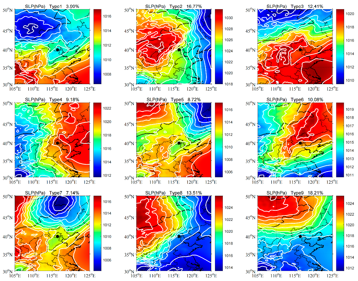
Using the T-model principal component analysis method to objectively analyze the daily SLP data at 00:00 every day from 1979 to 2021, we classified nine main circulation patterns in the eastern part of northern China. The average SLPs and occurrence frequencies for the circulation types are shown in Figure 1. According to the main weather systems that affect Beijing, as well as their locations and intensities, the nine circulation patterns were: low pressure in the northwest (CT1), high-pressure front (CT2), high-pressure system (CT3), high-pressure rear (CT4), low pressure in the northeast (CT5), high pressure in the northeast (CT6), weak pressure field or equalizing field (CT7), high pressure in the northwest (CT8), and high pressure in the north (CT9). Among these patterns, CT2, CT3, CT8, and CT9 comprised 16.77%, 12.41%, 13.51%, and 18.21%, respectively, which were the main circulation patterns.
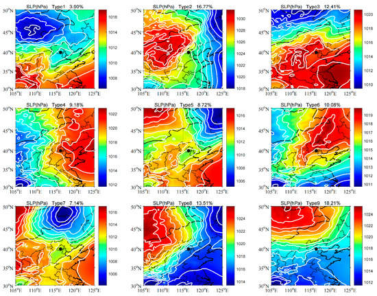
Figure 1.
Primary circulation patterns in Beijing from 1979 to 2021. Black dots indicate the location of Beijing in all panels. White contour lines represent SLP values (hPa). Filled color contours represent the air pressure distribution.
Figure 2 shows the monthly distributions of the nine circulation patterns, indicating that CT2 and CT9 occurred most frequently in February, accounting for ~48% of the total. These two circulation patterns correspond to the location of the cold high-pressure systems over Beijing during the winter and the northeast and northwest cold airflow paths to the south.
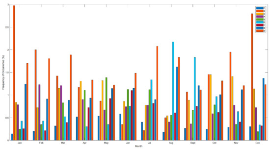
Figure 2.
Monthly occurrence distributions of each circulation pattern (labeled 1–9) in Beijing.
3.2. Relationships between Circulation Patterns and Pollutant Concentrations
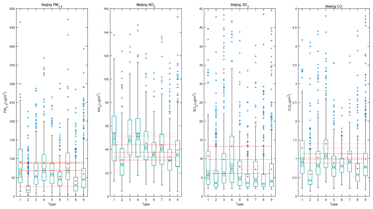
Figure 3 shows the distributions of PM2.5, NO2, SO2, and CO concentrations in Beijing under the nine circulation types (daily average concentrations). The pollutant concentrations were obtained by averaging the data at each monitoring station.
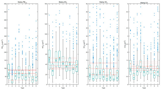
Figure 3.
Box-plots of PM2.5, NO2, SO2, and CO concentrations corresponding to the nine circulation types (CT on the x-axis) in Beijing from 2015 to 2021. The dots indicate mean values, whereas the bottoms and tops of the dashed lines represent the values of the 5th and 95th percentiles, respectively. The lower sides of the boxes represent the 25th percentile, the middle lines (red) represent the medians, and the upper lines represent the 75th percentile. Red crosses indicate outliers.
Figure 3 shows that, under the CT1, CT4, and CT7 patterns, the PM2.5 concentrations in Beijing were higher, with average values of 90.57 μg m−3, 88.32 μg m−3, and 86.53 μg m−3, respectively. Under the CT2 and CT8 patterns, the PM2.5 concentrations were lower, with average values of 26.82 μg m−3 and 41.46 μg m−3, respectively. For NO2, under the CT1, CT3, and CT4 patterns, the NO2 concentrations in Beijing were relatively high (54.07 μg m−3, 51.38 μg m−3, and 53.51 μg m−3, respectively), while the concentrations under the CT2 and CT8 patterns were relatively low (30.13 μg m−3 and 33.37 μg m−3, respectively). Under the CT1, CT3, and CT4 patterns, the SO2 concentrations were higher (10.67 μg m−3, 9.76 μg m−3, and 13.28 μg m−3, respectively), while the SO2 concentrations under the CT2, CT6, and CT8 patterns were lower (6.11 μg m−3, 5.21 μg m−3, and 5.94 μg m−3, respectively). The distributions of CO and NO2 were similar. Under the CT1, CT3, and CT4 patterns, the CO concentrations in Beijing were higher, while those under the CT2 and CT8 patterns were lower.
3.3. FLEXPART-WRF Simulation Results
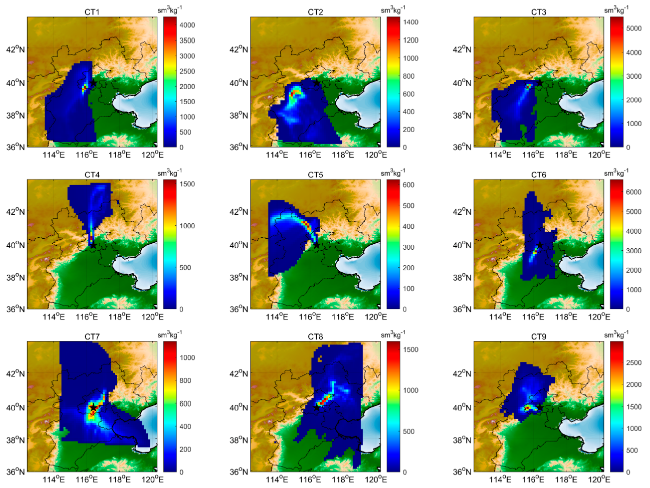
We selected the serious pollution events (highest PM2.5 concentrations) for the nine circulation patterns from 2015 to 2021 and used the FLEXPART-WRF model to conduct 48 h backward simulations to study the residence times of the pollutant unit concentrations and estimate their impacts on the Beijing area. The footprint analysis results are shown in Figure 4.

Figure 4.
Total footprints (residence times of 48 h backward trajectories) for the most severe haze events that occurred under the nine circulation types from 2015 to 2021. The unit means the residence time of particles per unit concentration. The solid black line in the figure is the administrative division map, and the area where the black star is located in the area of Beijing.
Figure 4 indicates that, under the influence of CT1, the particles mainly resided in the southwestern part of Beijing, which roughly corresponds to the low-pressure location in this circulation pattern. The particles also had the longest residence times in the area of Beijing. The residence time of the particles per unit concentration exceeded one hour. When Beijing was influenced by CT2, the particle residence time was generally short, and the longest residence time within 48 h was only 20 min. Under the influence of CT3, the particles were also concentrated in the western part of Beijing. The residence time of the unit particles in the area of Beijing was more than 1.5 h, which is longer than that of CT1. Under the influence of CT4, the pollutant particles affecting Beijing came from the north. Although their average residence times were small, they remained in a large area of Beijing for more than 30 min. Therefore, under the influence of CT4, the pollutant particles did not diffuse easily, thereby causing the pollutant concentrations to increase. Under the influence of CT5, Beijing’s diffusion conditions were relatively good, and the pollutant residence time was relatively short. The maximum residence time within 48 h was less than 10 min; therefore, the corresponding pollutant concentrations were relatively low. When Beijing was influenced by CT6, the city was generally controlled by high pressure. Pollutants remained in the southwestern part of the area for an extended period, and those that remained for more than 1 h were mainly concentrated outside Beijing. Thus, the pollutant concentrations under the CT6 pattern were relatively low. When Beijing was influenced by CT7, although the total residence time was short, the particles remained in the area of Beijing, and the corresponding pollutant concentrations were relatively high. Under the influence of CT8 and CT9, the pollutant residence times ranged from 500 to 1500 sm3kg−1, and most particles were not in the area of Beijing; therefore, the pollutant concentrations corresponding to these two circulation patterns were low.
4. Discussion: Air Quality Forecast during the Winter Olympics
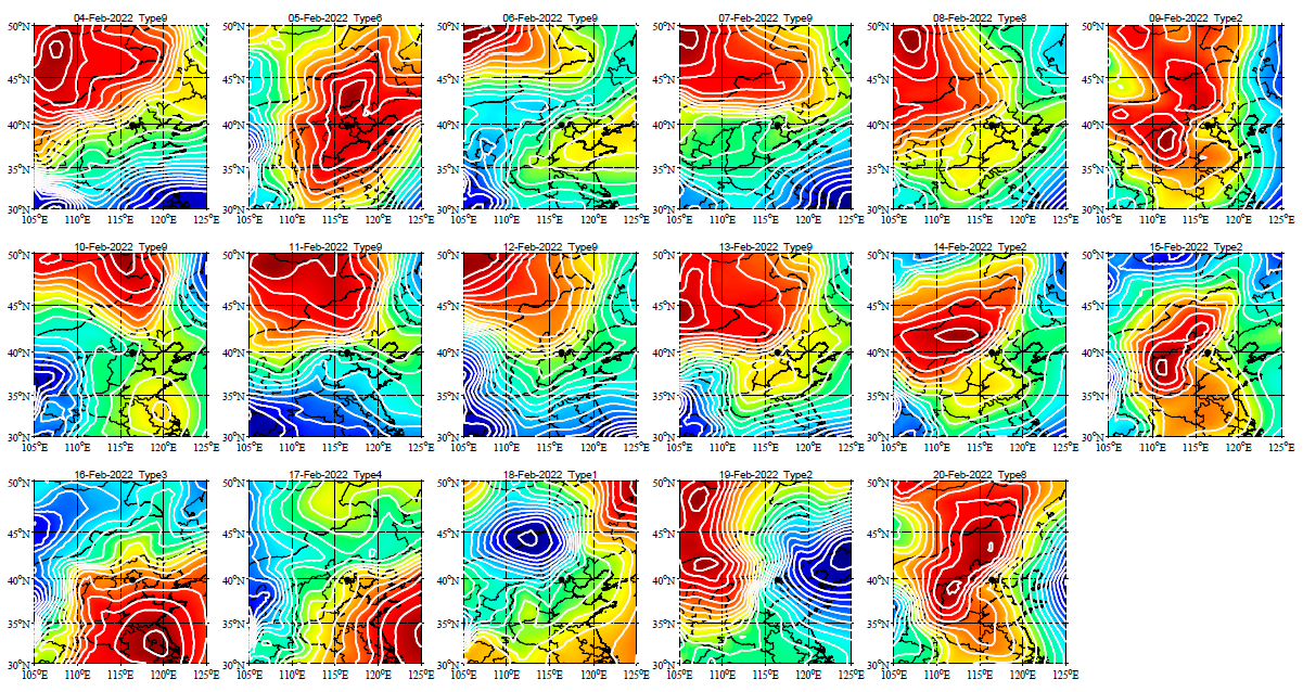
According to the predictions of the EC-Earth forecast model, the distribution of SLP in Beijing during the Winter Olympics was obtained. The daily circulation forecast are shown in Figure 5.
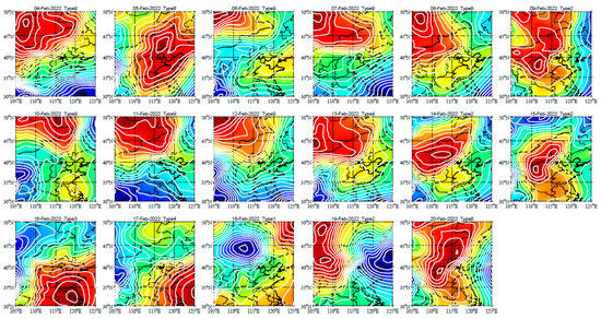
Figure 5.
Daily sea level pressure (SLP) patterns during the 2022 Winter Olympics.
Comparing the pressure field predicted by the EC-Earth model with the circulation patterns, the corresponding daily circulation patterns are listed in Figure 5. We predicted that, during the Winter Olympics, the predominant circulation patterns were CT9 (7 d), CT2 (4 d), and CT8 (2 d), with CT1, CT3, CT4, and CT6 each occurring for one day. We determined that the three-day circulation patterns (CT3, CT4, and CT1) on the 16th, 17th, and 18th of February corresponded to high pollutant concentrations. We then calculated the median, average, and standard deviations of the four pollutant concentrations between February 2015–2021 (Table 2). The pollutant concentration distributions in February for each circulation pattern were similar to the annual distribution (Figure 3). The pollutant concentrations corresponding to CT1, CT3, and CT4 were all higher than that of CT2, CT6, CT8, and CT9.
Table 2.
Statistics of pollutant concentrations in Beijing from 2015 to 2021.
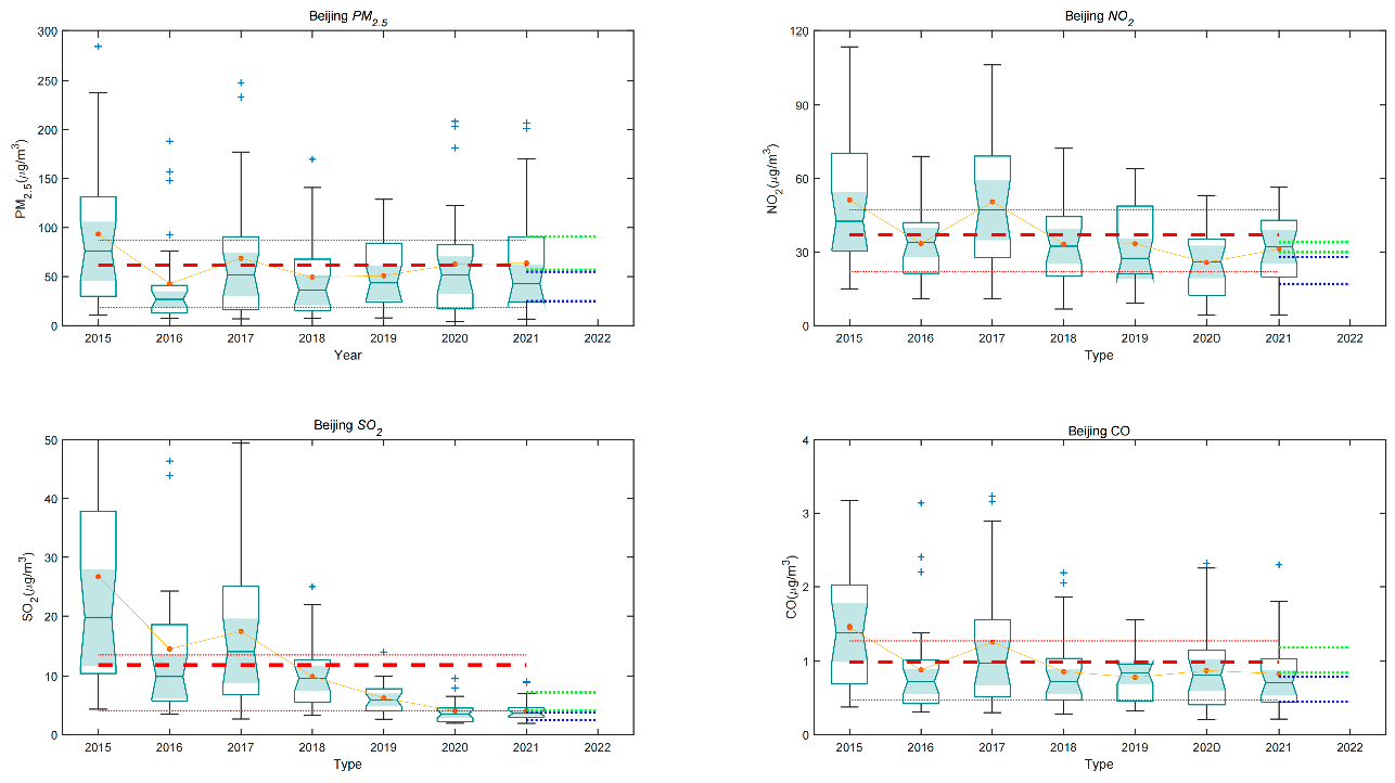
We calculated the trends for the four pollutants from 2015 to 2021 (Figure 6). For the past three years, the overall PM2.5 and CO concentrations increased from 2019 to 2020, and then decreased from 2020 to 2021. Although Beijing was affected by lockdown due to the COVID-19 pandemic in 2020, resulting in reduced emissions caused by human activity, the city’s meteorological conditions were not conducive to the diffusion of PM2.5 and CO [41,42], which likely led to higher pollutant concentrations in 2020 compared to 2019. It is expected that the Beijing Municipal Government will further control emissions during the 2022 Winter Olympics [43,44]. In addition, the circulation conditions during the Winter Olympics should generally be conducive to diffusing pollutants. Therefore, we predict that during February 2022, the PM2.5 and CO concentrations will be similar to those in 2019. Calculating the decreasing ratio of the average concentrations in 2019 to the seven-year average concentrations, we found that PM2.5 would decrease by ~17.4%, while CO would decrease by ~21.2%.
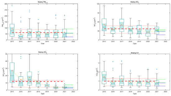
Figure 6.
Pollutant distributions in Beijing during February of 2015–2021. The thicker red dash line represents the 2015–2021 average, and the thinner red dash line represents the 2015–2021 quartile. The green dash line shows the predicted range of 17–19 days during the Winter Games, and the blue dash line shows the range of other days during the Winter Games.
The NO2 and SO2 trends were the opposite of those of PM2.5 and CO. They decreased from 2019 to 2020 and then increased from 2020 to 2021. Due to the influence of the height of the boundary layer in 2020 [45], both concentrations were lower than in 2019. In February 2021, Beijing was not affected by lockdown, and emissions increased, resulting in a slight increase in the concentrations of these two pollutants. During the Winter Olympics, because Beijing will further control emissions, we expect that the NO2 concentration may keep decreasing, as it did from 2019 to 2020, which was 34.59% lower than the seven-year average. Comparing the SO2 average concentrations in 2020 and 2021, we found that, although the concentration increased slightly in 2021, the magnitude of this increase was small. Therefore, we expect that the average SO2 concentration in 2022 will maintain the 2020 and 2021 average, which was 65.64% lower than the seven-year average.
By combining the average pollutant concentrations under each circulation pattern and the trends for the past seven years, we expect that the air quality during the 2022 Winter Olympics will be good if the Beijing municipal government takes reasonable measures to control emissions. The concentrations of PM2.5, NO2, SO2, and CO will likely be higher from the 17th to the 19th February 2022, with overall predicted ranges of 57–91 μg m−3, 30–34 μg m−3, 4.1–7.2 μg m−3, and 0.85–1.19 mg m−3, respectively. For the rest of the Olympics, the PM2.5, NO2, SO2, and CO concentrations are predicted to have ranges of 25–55 μg m−3, 17–28 μg m−3, 2.5–3.8 μg m−3, and 0.45–0.79 mg m−3, respectively. The intuitive range is shown in Figure 6.
Figure S1 showed the trend of PM2.5 and CO concentrations during the Beijing Winter Olympic Games (2022.02.04–2022.02.20). Figure S2 showed the trend of NO2 and SO2 concentrations during the Beijing Winter Olympic Games (2022.02.04–2022.02.20). Table S1 shows the concentration range and mean values of PM2.5, NO2, SO2, and CO during the Beijing Winter Olympics and from 2.17 to 2.19 (2022). By comparing the monitoring data and the prediction results, we found that the average measured pollutant concentration was in the range of our prediction (Table S1). The expected period of bad air quality (2.17–2.19) also shows the trend of increasing pollutant concentration, but the average pollutant concentration during this period is less than or near the lower limit of the prediction results. In the meanwhile, we found that pollutant concentrations were also higher during 9th–14th. Therefore, our prediction results are partially effective, roughly better reflecting the overall situation of pollutant concentration during the Beijing Winter Olympics, and partially accurate for the prediction of pollution weather.
5. Conclusions
The surface pressure field in Beijing from 1979 to 2021 was classified, and the atmospheric circulation patterns affecting Beijing were divided into nine types. We found that the circulation patterns were closely related to air quality. When Beijing was controlled by CT1, CT4, and CT7, the PM2.5 concentrations were higher, and when it was controlled by CT1, CT3, and CT4, the NO2, SO2, and CO concentrations were higher. The concentrations of all four pollutants were lower under the influence of CT2 and CT8.
Using the FLEXPART-WRF model to simulate the 48 h backward particle trajectories using the highest PM2.5 concentrations for each of the circulation patterns, the residence times of the unit concentrations were calculated. We found that the circulation patterns with higher average PM2.5 concentrations had longer particle residence times in Beijing.
By comparing the predicted surface pressure results obtained from the climate model for the period of the 2022 Winter Olympics, we found that the circulation pattern in Beijing during the Winter Olympics is expected to generally be conducive to diffusing pollutants and good air quality. Pollutant accumulation would only occur under circulation patterns CT1, CT3, and CT4 on 17–19 February 2022. By using the trends in pollutant changes during the past seven years, we predicted that the corresponding PM2.5, NO2, SO2, and CO concentrations would be higher from 17–19 February, with ranges of 57–91 μg m−3, 30–34 μg m−3, 4.1–7.2 μg m−3, and 0.85–1.19 mg m−3, respectively. For the rest of the Olympics, the corresponding PM2.5 NO2, SO2, and CO concentrations were predicted to have ranges of 25–55 μg m−3, 17–28 μg m−3, 2.5–3.8 μg m−3, and 0.45–0.79 mg m−3.
By evaluating the prediction results from the monitoring data, we found that the predictions were generally reliable, and the overall air quality during the Beijing Winter Olympic Games was good. There are two main periods with high pollutant concentrations (9th–14th and 17th–19th, respectively), and we effectively predicted the small range of bad air quality occurring during 17th–19th due to weather conditions. It Demonstrated that our predictive means are partially effective but still require improvement.
Based on the prediction results of this approach, the government could adjust the emission strategy for the time when the circulation and diffusion conditions are expected to be poor so as to ensure good air quality during the Winter Olympics. In addition, this method can be extended to other fields and events so as to better assist the government in making decisions on air quality.
Supplementary Materials
The following supporting information can be downloaded at: https://www.mdpi.com/article/10.3390/su14084574/s1, Figure S1: Trend of PM2.5 and CO concentrations during the Beijing Winter Olympic Game (2022.02.04–2022.02.20); Figure S2: Trend of NO2 and SO2 concentrations during the Beijing Winter Olympic Games (2022.02.04–2022.02.20); Table S1: Concentration range and mean values of PM2.5, NO2, SO2, and CO during the Beijing Winter Olympics and during 2.17–2.19 (2022).
Author Contributions
Data curation, J.Z.; methodology, J.Z.; project administration, C.Z.; resources, Z.Z. (Zeming Zhou); software, H.D.; supervision, H.X.; visualization, H.D.; writing—original draft, Z.Z. (Zezheng Zhao) and T.W.; writing—review and editing, A.R. and C.Z. All authors have read and agreed to the published version of the manuscript.
Funding
This research was funded by [National Key R&D Program of China] grant number [2017YFC1501803].
Institutional Review Board Statement
Not applicable.
Informed Consent Statement
Not applicable.
Data Availability Statement
The data that support the findings of this study is available at this site (https://doi.org/10.5281/zenodo.5146851 (accessed on 29 July 2021)).
Acknowledgments
This study was supported by the National Key R&D Program of China (2017YFC1501803). We thank the authors and developers of the COST733 classification software.
Conflicts of Interest
The authors declare no conflict of interest.
References
- Dayan, U.; Levy, I. Relationship between synoptic-scale atmospheric circulation and ozone concentrations over Israel. J. Geophys. Res. Earth Surf. 2002, 107, 4813. [Google Scholar] [CrossRef]
- Santurtún, A.; González-Hidalgo, J.C.; Sanchez-Lorenzo, A.; Zarrabeitia, M.T. Surface ozone concentration trends and its relationship with weather types in Spain (2001–2010). Atmos. Environ. 2015, 101, 10–22. [Google Scholar] [CrossRef]
- Zhou, C.; Wei, G.; Xiang, J.; Zhang, K.; Li, C.; Zhang, J. Effects of synoptic circulation patterns on air quality in Nanjing and its surrounding areas during 2013–2015. Atmos. Pollut. Res. 2018, 9, 723–734. [Google Scholar] [CrossRef]
- Tian, Y.; Jiang, Y.; Liu, Q.; Xu, D.; Zhao, S.; He, L.; Liu, H.; Xu, H. Temporal and spatial trends in air quality in Beijing. Landsc. Urban Plan. 2019, 185, 35–43. [Google Scholar] [CrossRef]
- Wu, L.; Li, N.; Yang, Y. Prediction of air quality indicators for the Beijing-Tianjin-Hebei region. J. Clean. Prod. 2018, 196, 682–687. [Google Scholar] [CrossRef]
- Russo, A.; Sousa, P.; Durão, R.; Ramos, A.; Salvador, P.; Linares, C.; Díaz, J.; Trigo, R. Saharan dust intrusions in the Iberian Peninsula: Predominant synoptic conditions. Sci. Total Environ. 2020, 717, 137041. [Google Scholar] [CrossRef]
- Russo, A.; Trigo, R.; Martins, H.; Mendes, M.T. NO2, PM10 and O3 urban concentrations and its association with circulation weather types in Portugal. Atmos. Environ. 2014, 89, 768–785. [Google Scholar] [CrossRef]
- Zhao, Z.; Xi, H.; Russo, A.; Du, H.; Gong, Y.; Xiang, J.; Zhou, Z.; Zhang, J.; Li, C.; Zhou, C. The Influence of Multi-Scale Atmospheric Circulation on Severe Haze Events in Autumn and Winter in Shanghai, China. Sustainability 2019, 11, 5979. [Google Scholar] [CrossRef] [Green Version]
- Zhou, C.; Wei, G.; Zheng, H.; Russo, A.; Li, C.; Du, H.; Xiang, J. Effects of potential recirculation on air quality in coastal cities in the Yangtze River Delta. Sci. Total Environ. 2019, 651, 12–23. [Google Scholar] [CrossRef]
- Han, Y.; Qi, M.; Chen, Y.; Shen, H.; Liu, J.; Huang, Y.; Chen, H.; Liu, W.; Wang, X.; Liu, J.; et al. Influences of ambient air PM2.5 concentration and meteorological condition on the indoor PM2.5 concentrations in a residential apartment in Beijing using a new approach. Environ. Pollut. 2015, 205, 307–314. [Google Scholar] [CrossRef]
- Ma, T.; Duan, F.; He, K.; Qin, Y.; Tong, D.; Geng, G.; Liu, X.; Li, H.; Yang, S.; Ye, S.; et al. Air pollution characteristics and their relationship with emissions and meteorology in the Yangtze River Delta region during 2014–2016. J. Environ. Sci. 2019, 83, 8–20. [Google Scholar] [CrossRef]
- Miao, Y.; Liu, S.; Guo, J.; Yan, Y.; Huang, S.; Zhang, G.; Zhang, Y.; Lou, M. Impacts of meteorological conditions on wintertime PM2.5 pollution in Taiyuan, North China. Environ. Sci. Pollut. Res. 2018, 25, 21855–21866. [Google Scholar] [CrossRef]
- Pucer, J.F.; Štrumbelj, E. Impact of changes in climate on air pollution in Slovenia between 2002 and 2017. Environ. Pollut. 2018, 242, 398–406. [Google Scholar] [CrossRef]
- Dong, Y.; Li, J.; Guo, J.; Jiang, Z.; Chu, Y.; Chang, L.; Yang, Y.; Liao, H. The impact of synoptic patterns on summertime ozone pollution in the North China Plain. Sci. Total Environ. 2020, 735, 139559. [Google Scholar] [CrossRef]
- Mao, F.; Zang, L.; Wang, Z.; Pan, Z.; Zhu, B.; Gong, W. Dominant synoptic patterns during wintertime and their impacts on aerosol pollution in Central China. Atmos. Res. 2020, 232, 104701. [Google Scholar] [CrossRef]
- Pandey, P.; Kumar, D.; Prakash, A.; Masih, J.; Singh, M.; Kumar, S.; Jain, V.K.; Kumar, K. A study of urban heat island and its association with particulate matter during winter months over Delhi. Sci. Total Environ. 2012, 414, 494–507. [Google Scholar] [CrossRef]
- Bei, N.; Li, G.; Huang, R.J.; Cao, J.; Meng, N.; Feng, T.; Liu, S.; Zhang, T.; Zhang, Q.; Molina, L.T. Typical synoptic situations and their impacts on the wintertime air pollution in the Guanzhong basin, China. Atmos. Chem. Phys. 2016, 16, 7373–7387. [Google Scholar] [CrossRef] [Green Version]
- Brioude, J.; Arnold, D.; Stohl, A.; Cassiani, M.; Morton, D.; Seibert, P.; Angevine, W.; Evan, S.; Dingwell, A.; Fast, J.D.; et al. The Lagrangian particle dispersion model FLEXPART-WRF version 3.1. Geosci. Model Dev. 2013, 6, 1889–1904. [Google Scholar] [CrossRef] [Green Version]
- Hazeleger, W.; Severijns, C.; Semmler, T.; Ştefănescu, S.; Yang, S.; Wang, X.; Wyser, K.; Dutra, E.; Baldasano, J.M.; Bintanja, R.; et al. EC-Earth. Bull. Am. Meteorol. Soc. 2010, 91, 1357–1364. [Google Scholar] [CrossRef] [Green Version]
- Huth, R. Properties of the circulation classification scheme based on the rotated principal component analysis. Meteorol. Atmos. Phys. 1996, 59, 217–233. [Google Scholar] [CrossRef]
- Huth, R.; Beck, C.; Philipp, A.; Demuzere, M.; Ustrnul, Z.; Cahynová, M.; Kyselý, J.; Tveito, O.E. Classifications of Atmospheric Circulation Patterns. Ann. N. Y. Acad. Sci. 2008, 1146, 105–152. [Google Scholar] [CrossRef] [PubMed]
- Philipp, A.; Bartholy, J.; Beck, C.; Erpicum, M.; Esteban, P.; Fettweis, X.; Huth, R.; James, P.; Jourdain, S.; Kreienkamp, F.; et al. Cost733cat—A database of weather and circulation type classifications. Phys. Chem. Earth Parts A/B/C 2010, 35, 360–373. [Google Scholar] [CrossRef]
- Zhang, J.P.; Zhu, T.; Zhang, Q.H.; Li, C.C.; Shu, H.L.; Ying, Y.; Dai, Z.P.; Wang, X.; Liu, X.Y.; Liang, A.M.; et al. The impact of circulation patterns on regional transport pathways and air quality over Beijing and its surroundings. Atmos. Chem. Phys. 2012, 12, 5031–5053. [Google Scholar] [CrossRef] [Green Version]
- Li-Juan, M.; Miao, L.-J.; Jiang, Z.-H.; Wang, G.-J.; Gnyawali, K.R.; Zhang, J.; Zhang, H.; Fang, K.; He, Y.; Li, C. Projected drought conditions in Northwest China with CMIP6 models under combined SSPs and RCPs for 2015–2099. Adv. Clim. Chang. Res. 2020, 11, 210–217. [Google Scholar] [CrossRef]
- You, Q.; Cai, Z.; Wu, F.; Jiang, Z.; Pepin, N.; Shen, S.S.P. Temperature dataset of CMIP6 models over China: Evaluation, trend and uncertainty. Clim. Dyn. 2021, 57, 17–35. [Google Scholar] [CrossRef]
- Balsamo, G.; Beljaars, A.; Scipal, K.; Viterbo, P.; van den Hurk, B.; Hirschi, M.; Betts, A.K. A Revised Hydrology for the ECMWF Model: Verification from Field Site to Terrestrial Water Storage and Impact in the Integrated Forecast System. J. Hydrometeorol. 2009, 10, 623–643. [Google Scholar] [CrossRef]
- Madec, G. NEMO Ocean Engine. Note du Pole de Modelisation; Institut Pierre-Simon Laplace (IPSL): Paris, France, 2008; No 27; ISSN 1288-1619. [Google Scholar] [CrossRef]
- Vancoppenolle, M.; Bouillon, S.; Fichefet, T.; Goosse, H.; Lecomte, O.; Morales Maqueda, M.A.; Madec, G. The Louvain-la-Neuve Sea Ice Model. Notes du pole de modélisation; Institut Pierre-Simon Laplace (IPSL): Paris, France, 2012; p. 31. [Google Scholar]
- Bothe, O.; Jungclaus, J.H.; Zanchettin, D. Consistency of the multi-model CMIP5/PMIP3-past1000 ensemble. Clim. Past 2013, 9, 2471–2487. [Google Scholar] [CrossRef] [Green Version]
- Atwood, A.R.; Wu, E.; Frierson, D.; Battisti, D.S.; Sachs, J.P. Quantifying Climate Forcings and Feedbacks over the Last Millennium in the CMIP5–PMIP3 Models. J. Clim. 2016, 29, 1161–1178. [Google Scholar] [CrossRef]
- Thomson, A.M.; Calvin, K.V.; Smith, S.J.; Kyle, G.P.; Volke, A.; Patel, P.; Delgado-Arias, S.; Bond-Lamberty, B.; Wise, M.A.; Clarke, L.E.; et al. RCP4.5: A pathway for stabilization of radiative forcing by 2100. Clim. Chang. 2011, 109, 77–94. [Google Scholar] [CrossRef] [Green Version]
- Yang, C.; Christensen, H.M.; Corti, S.; von Hardenberg, J.; Davini, P. The impact of stochastic physics on the El Niño Southern Oscillation in the EC-Earth coupled model. Clim. Dyn. 2019, 53, 2843–2859. [Google Scholar] [CrossRef] [Green Version]
- Bilbao, R.; Wild, S.; Ortega, P.; Acosta-Navarro, J.; Arsouze, T.; Bretonnière, P.-A.; Caron, L.-P.; Castrillo, M.; Cruz-García, R.; Cvijanovic, I.; et al. Assessment of a full-field initialized decadal climate prediction system with the CMIP6 version of EC-Earth. Earth Syst. Dyn. 2021, 12, 173–196. [Google Scholar] [CrossRef]
- Zhang, Q.; Berntell, E.; Li, Q.; Ljungqvist, F.C. Understanding the variability of the rainfall dipole in West Africa using the EC-Earth last millennium simulation. Clim. Dyn. 2021, 57, 93–107. [Google Scholar] [CrossRef]
- Hersbach, H.; Bell, B.; Berrisford, P.; Hirahara, S.; Horanyi, A.; Muñoz-Sabater, J.; Nicolas, J.; Peubey, C.; Radu, R.; Schepers, D.; et al. The ERA5 global reanalysis. Q. J. R. Meteorol. Soc. 2020, 146, 1999–2049. [Google Scholar] [CrossRef]
- Zhao, S.; Yu, Y.; Yin, D.; He, J.; Liu, N.; Qu, J.; Xiao, J. Annual and diurnal variations of gaseous and particulate pollutants in 31 provincial capital cities based on in situ air quality monitoring data from China National Environmental Monitoring Center. Environ. Int. 2016, 86, 92–106. [Google Scholar] [CrossRef]
- Cécé, R.; Bernard, D.C.; Brioude, J.; Zahibo, N. Microscale anthropogenic pollution modelling in a small tropical island during weak trade winds: Lagrangian particle dispersion simulations using real nested LES meteorological fields. Atmos. Environ. 2016, 139, 98–112. [Google Scholar] [CrossRef]
- Ghahremaninezhad, R.; Norman, A.-L.; Abbatt, J.P.D.; Levasseur, M.; Thomas, J.L. Biogenic, anthropogenic and sea salt sulfate size-segregated aerosols in the Arctic summer. Atmos. Chem. Phys. 2016, 16, 5191–5202. [Google Scholar] [CrossRef] [Green Version]
- Wentworth, G.R.; Murphy, J.G.; Croft, B.; Martin, R.V.; Pierce, J.R.; Côté, J.-S.; Courchesne, I.; Tremblay, J.; Gagnon, J.; Thomas, J.L.; et al. Ammonia in the summertime Arctic marine boundary layer: Sources, sinks, and implications. Atmos. Chem. Phys. 2016, 16, 1937–1953. [Google Scholar] [CrossRef] [Green Version]
- Ashbaugh, L.L.; Malm, W.C.; Sadeh, W.Z. A residence time probability analysis of sulfur concentrations at grand Canyon National Park. Atmos. Environ. 1985, 19, 1263–1270. [Google Scholar] [CrossRef]
- Brimblecombe, P.; Lai, Y. Diurnal and weekly patterns of primary pollutants in Beijing under COVID-19 restrictions. Faraday Discuss. 2021, 226, 138–148. [Google Scholar] [CrossRef]
- Sulaymon, I.D.; Zhang, Y.; Hopke, P.K.; Hu, J.; Zhang, Y.; Li, L.; Mei, X.; Gong, K.; Shi, Z.; Zhao, B.; et al. Persistent high PM2.5 pollution driven by unfavorable meteorological conditions during the COVID-19 lockdown period in the Beijing-Tianjin-Hebei region, China. Environ. Res. 2021, 198, 111186. [Google Scholar] [CrossRef]
- Liu, J. Strategies and Actions of Beijing 2022 Winter Olympics For Addressing Climate Change. Energy Conserv. Environ. Prot. 2021, 6, 5. (In Chinese) [Google Scholar]
- A Series of Press Conferences for the 2022 Winter Olympic and Paralympic Games—Special Ecological Environment. Environ. Life 2021, 12. (In Chinese). Available online: http://www.scio.gov.cn/xwfbh/xwbfbh/wqfbh/47673/47706/xgfbh47711/Document/1718851/1718851.htm (accessed on 5 April 2022).
- Hua, J.; Zhang, Y.; de Foy, B.; Shang, J.; Schauer, J.J.; Mei, X.; Sulaymon, I.D.; Han, T. Quantitative estimation of meteorological impacts and the COVID-19 lockdown reductions on NO2 and PM2.5 over the Beijing area using Generalized Additive Models (GAM). J. Environ. Manag. 2021, 291, 112676. [Google Scholar] [CrossRef] [PubMed]

Publisher’s Note: MDPI stays neutral with regard to jurisdictional claims in published maps and institutional affiliations. |
© 2022 by the authors. Licensee MDPI, Basel, Switzerland. This article is an open access article distributed under the terms and conditions of the Creative Commons Attribution (CC BY) license (https://creativecommons.org/licenses/by/4.0/).