Abstract
Owing to climate change, industrial pollution, and population gathering, the air quality status in many places in China is not optimal. The continuous deterioration of air-quality conditions has considerably affected the economic development and health of China’s people. However, the diversity and complexity of the factors which affect air pollution render air quality monitoring data complex and nonlinear. To improve the accuracy of prediction of the air quality index (AQI) and obtain more accurate AQI data with respect to their nonlinear and nonsmooth characteristics, this study introduces an air quality prediction model based on the empirical mode decomposition (EMD) of LSTM and uses improved particle swarm optimization (IPSO) to identify the optimal LSTM parameters. First, the model performed the EMD decomposition of air quality data and obtained uncoupled intrinsic mode function (IMF) components after removing noisy data. Second, we built an EMD–IPSO–LSTM air quality prediction model for each IMF component and extracted prediction values. Third, the results of validation analyses of the algorithm showed that compared with LSTM and EMD–LSTM, the improved model had higher prediction accuracy and improved the model fitting effect, which provided theoretical and technical support for the prediction and management of air pollution.
1. Introduction
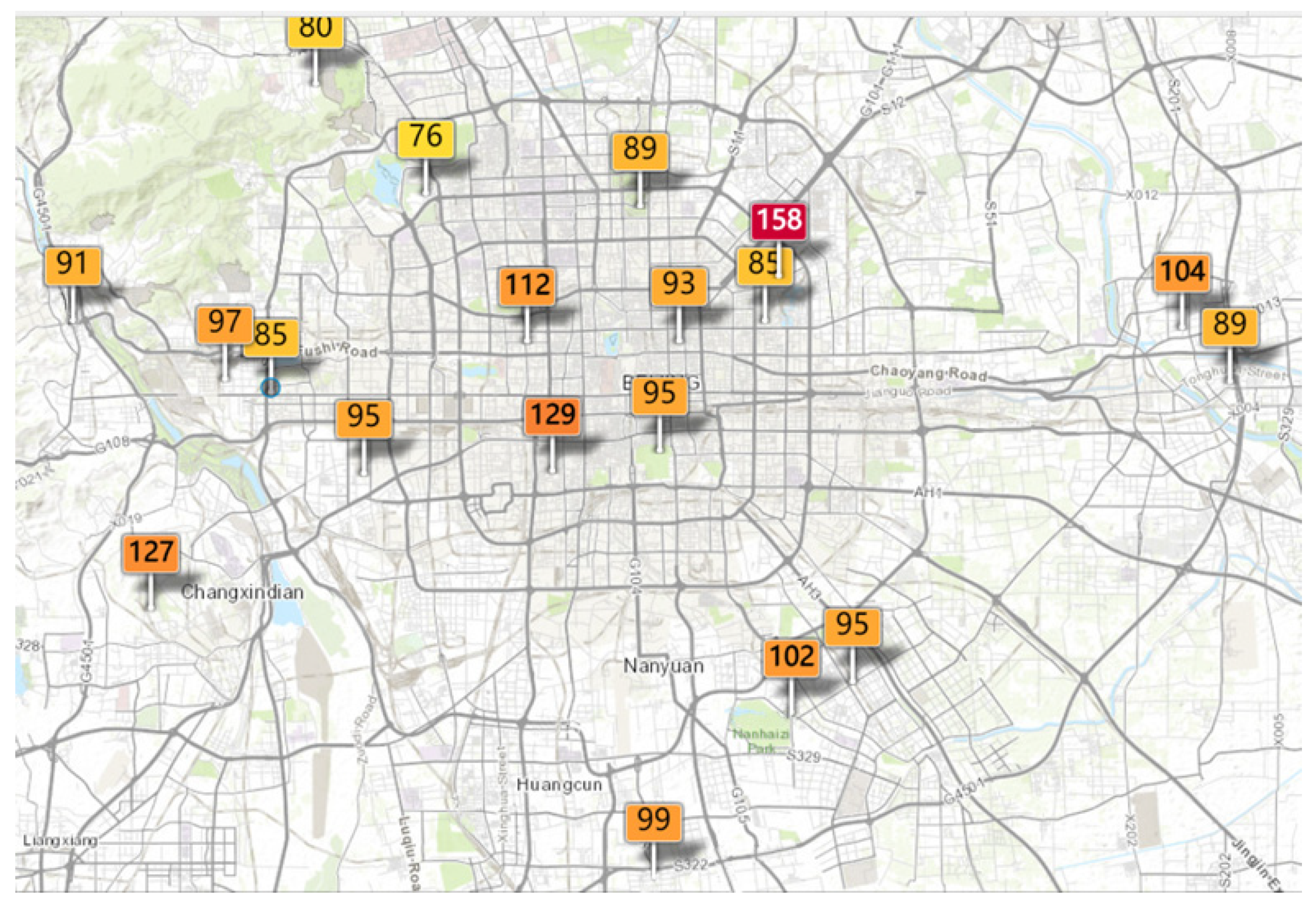
Aerial substances that are dangerous and serious to human health are collectively known as “air pollution” [1]. The Chinese economy’s rapid expansion and the growth in the number of cars and industries has increased air pollution and has become a serious problem [2]. Thus, most Chinese cities have established air-quality monitoring networks with the government’s help [3]. However, to solve the problem of air pollution, the important thing is not to monitor the air pollution in real-time, but to accurately predict the air quality, which helps cities develop and protect people’s health [4]. Figure 1 shows the air quality of Beijing on a specific day in 2020. The continually deteriorating air-quality conditions have seriously affected the economic development and human health of China. The air quality index (AQI) is an evaluation standard for the concentration of aerial pollutants. It is calculated from the concentration of the individual pollutants of SO2, NO2, PM10, PM2.5, CO, and O3 in the air, which enables people to have an intuitive understanding of air pollution. Table 1 shows the classification criteria for AQI. Research shows that there is an inevitable relationship between air pollution and respiratory diseases [5]. Polluted air mainly enters the human body through the respiratory system, which seriously affects human health. Accurate early warnings concerning the predicted level of air pollution are crucial to the prevention and control of air pollution as cities develop. Therefore, it is important to monitor and warn people about the air quality.
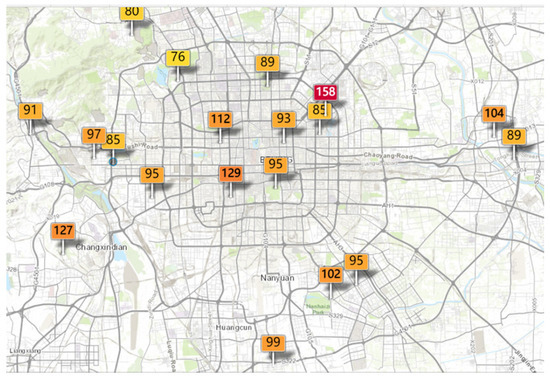
Figure 1.
AQI values of air-quality monitoring stations in Beijing on a specific day in 2020.

Table 1.
Classification criteria for AQI.
In the 1980s, mathematical and statistical prediction methods and numerical analyses were used to quantify pollutants [6]. The classic time series analysis is a standard statistical technique. The autoregressive, moving average, autoregressive moving average, and autoregressive integrated moving average (ARIMA) models are classical statistical models used in this field [7]. TRIPTI et al. [8] used the seasonal ARIMA (SARIMA) model and forecast future trends by making the data stationary. However, owing to the diversity of the factors affecting air pollution, air-quality monitoring data have complex characteristics which greatly influence the accurate prediction of air-quality. Nowadays, air quality has become increasingly important to people. An increasing number of research studies have been conducted on air quality [9]. Machine learning (ML) algorithms have been successfully applied to air-quality prediction by several researchers [10,11,12,13,14]. The support vector regression machine is a ML method used to minimize structural risk based on statistical learning theory [15]. Leong et al. [16] proposed a support vector machine (SVM) model to predict the air pollution index and showed that the model could solve the problem of air pollution using radial basis functions effectively and accurately. Wang et al. [17] proposed the new hybrid Garch method that combined the individual prediction model of ARIMA and SVM and generated reliable and accurate predictions. Traditional analysis methods are no longer suitable for processing a large amount of time series data. Du et al. [18] studied the periodic solution of a discrete-time neutral neural network. The study proved its stability and was extended to other neural networks. In recent years, neural networks such as biological neural networks and artificial neural networks have developed rapidly [19] and have been extensively used in the fields of image identification [20,21,22], stock price forecasting [23,24,25], intelligent robots [26,27,28], and elsewhere.
Recurrent neural networks (RNNs) have been extensively used for learning time series data, and long short-term memory (LSTM) neural networks enable RNN to learn long-term temporal dependencies. Seng et al. [29] proposed a comprehensive method of prediction based on LSTM with many environmental datasets. The results showed that LSTM solved the gradient disappearance and gradient explosion of RNN and achieved higher prediction accuracy, which verified that LSTM had good application prospects in time series prediction. Qadeer et al. [30] used different ML methods to predict hourly PM2.5 concentrations in two major cities in Korea. The results showed that the performance of an optimized LSTM network was superior to other models. Liu et al. [31] used a LSTM model based on factory-aware attention mechanism for PM2.5 predictions and showed that the obtained results were superior to other traditional ML methods for forecasting PM2.5 pollutants. Arsov et al. [32] used RNNs with memory units to forecast PM10 particulate matter concentrations and revealed that (a) the prediction effect of this model was better than the base model and (b) it could be successfully applied to the prediction of atmospheric pollution. Wang et al. [33] proposed a chi-square test (CT)-LSTM method which combined the CT and a LSTM network model to build a predictive model. The results showed that the air quality data could be further analyzed from the aspect of data preprocessing in future work to improve prediction accuracy. In recent years, wavelet decomposition has been used for data enhancement in deep learning. Sheen Mclean et al. [34] proposed a new spatiotemporal interpolation model which combined deep learning with wavelet preprocessing technology. The overall results showed that the latest model proposed exhibited great potential in the assessment of the spatiotemporal characteristics of outdoor air pollution. Huang et al. [35] used the combination of empirical mode decomposition (EMD) and gated recurrent unit to predict PM2.5 concentration, and the study showed that the prediction result was greatly improved compared with the single model. This work showed that EMD could use decomposition and reconstruction to improve the prediction accuracy of the model when dealing with complex air quality data.
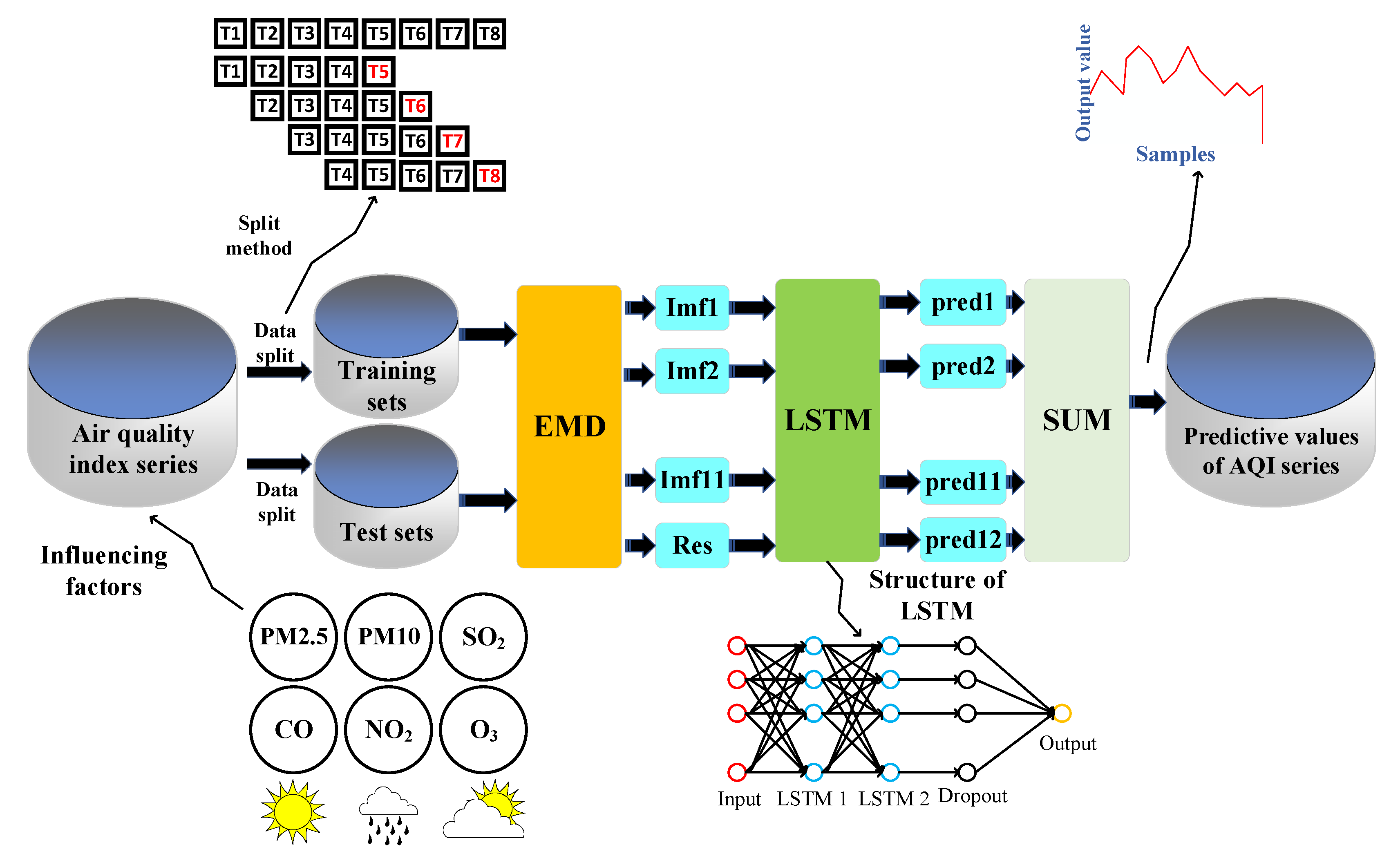
Based on the above, an air-quality prediction method combined with EMD–IPSO–LSTM is proposed here to improve the predictive accuracy of the air-quality index (AQI). Figure 2 shows a general overview of the research methodology. First, EMD was mainly used to extract all the scales of the original signal. Second, the extracted components with different frequencies were input in the LSTM model for training. Subsequently, the numbers of neurons in each LSTM layer were determined by the improved particle swarm optimization (IPSO) algorithm. Third, the latest model was used to conduct experiments on the AQI for data from Beijing acquired from 1 January 2020 to 31 December 2020.
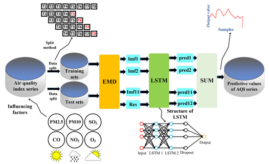
Figure 2.
Research method and overall structure.
This paper’s contributions are:
(1) Since EMD can decompose time series data into multiple signals of different frequencies, training each signal separately can make complex time series data easier to predict, so we used EMD decomposition to decompose the AQI data. The decomposed multiple smooth subsequences were then input in the constructed LSTM model. Finally, results were acquired by summarizing all the sequences predicted by the LSTM. (2) Given that the parameters of the LSTM model are mostly set empirically, the IPSO algorithm was used to solve the optimal parameters. (3) A nonlinear decreasing inertia weight and a learning factor that changes with the inertia weight are proposed to overcome the problems of standard PSO associated with the fact that it is easy to fall into local optima and slow convergence at the later stage. (4) Model training was conducted at representative locations in Beijing to prove the universality of the model. (5) The model was compared with the single LSTM and EMD–LSTM model, and the experimental results show that each evaluation index has been significantly improved, which proves the model’s effectiveness.
This paper is organized as follows. Section 1 introduces the definition of air quality index and expounds the research status of air quality. In view of the shortcomings of previous work, we analyze the progress of relevant research work and demonstrate the main contribution of this paper. Section 2 introduces the main techniques used in this paper and the relevant theories are described in detail. Section 3 introduces the data source and the method of data preprocessing. In addition, the experimental setup and research process are described, and the research results are recorded. Section 4 summarizes this paper and discusses the results obtained. At the same time, it also discusses the shortcomings of this work and provides research ideas for future work. Section 5 summarizes the results of this study and draws a conclusion which verifies the contribution of this paper to air quality prediction.
2. Materials and Methods
2.1. Principle of EMD
As an adaptive signal decomposition method, EMD was extensively used to decompose time series into multiple intrinsic mode function (IMF) and a residual component [36,37,38]. In turn, the IMF components were determined by satisfying two conditions:
- (1)
- The number of extreme and zero points had to be equal to or differ by no more than one.
- (2)
- For each time series, the average value of the upper envelope formed by the local maximum value and the lower envelope formed by the local minimum value was zero.
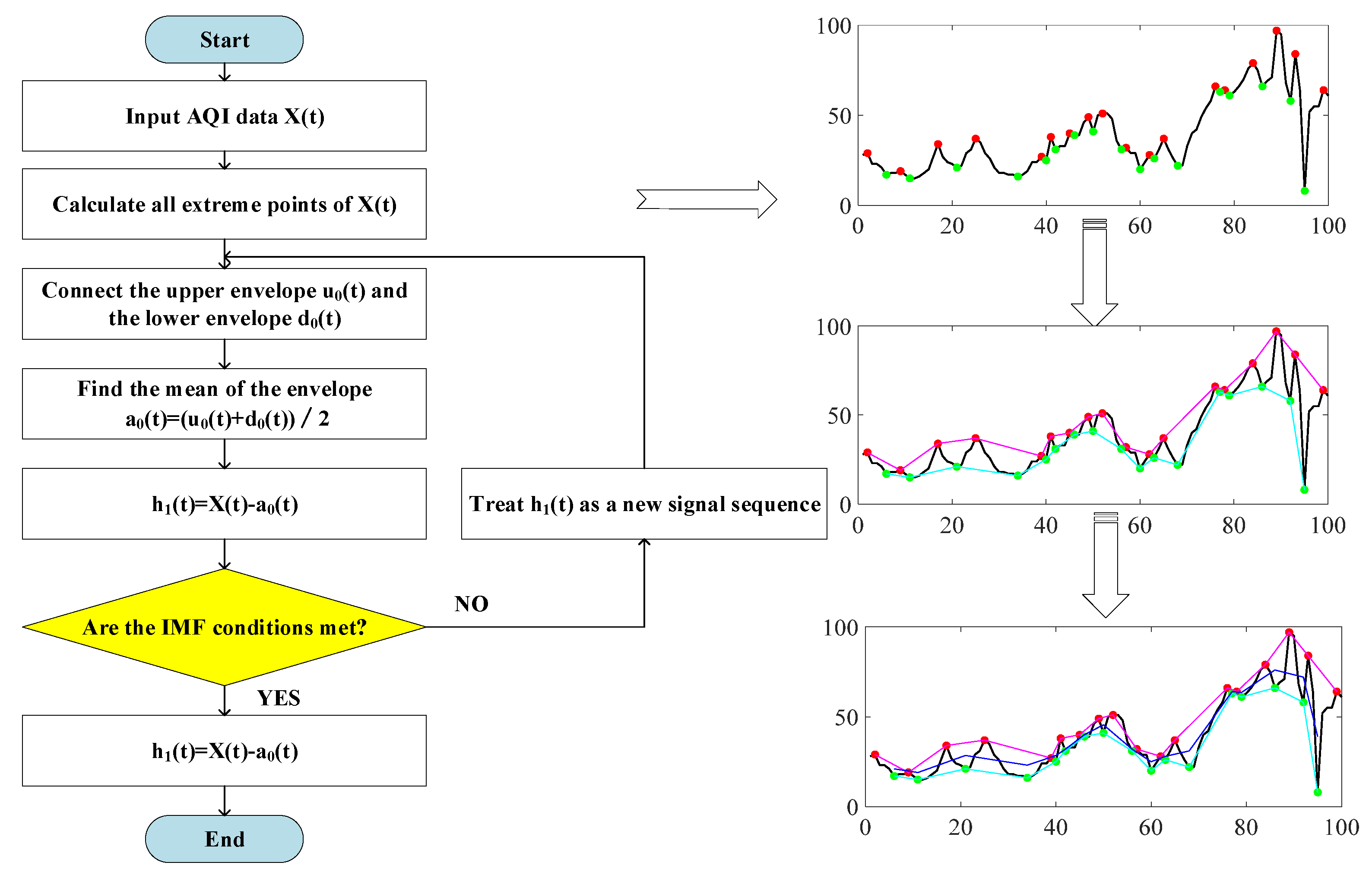
Figure 3 shows the flow of the specific decomposition method of EMD. The specific decomposition method was:
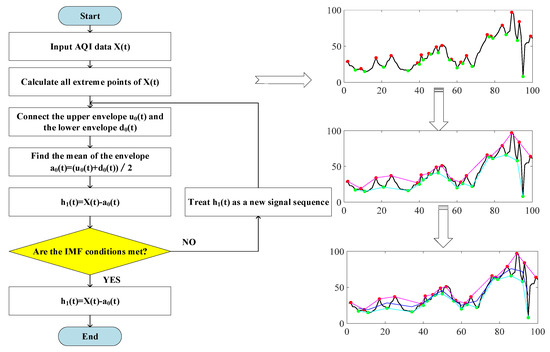
Figure 3.
Flow chart of the EMD method.
- (1)
- Identify all local maxima and local minima of the sequence to be decomposed and connect all local maxima and local minima to form the upper envelope and the lower envelope , respectively.
- (2)
- Identify the mean value of the upper and lower envelopes, and subtract the mean value from the sequence to be decomposed to obtain the component , i.e., .
- (3)
- Determine whether satisfied the IMF condition. If it was satisfied, was the first IMF component. However, if the condition was not satisfied, apply the same processing to as that applied to . The new component would be judged and processed in the same way until the IMF conditions were met. The first component of IMF would then be obtained.
- (4)
- Repeat the above steps with the remaining component as a new decomposition sequence until the component or the remaining component was less than the predetermined value or the remaining component became a monotonic function. The final result was . The decomposition of the original sequence was completed at this point.
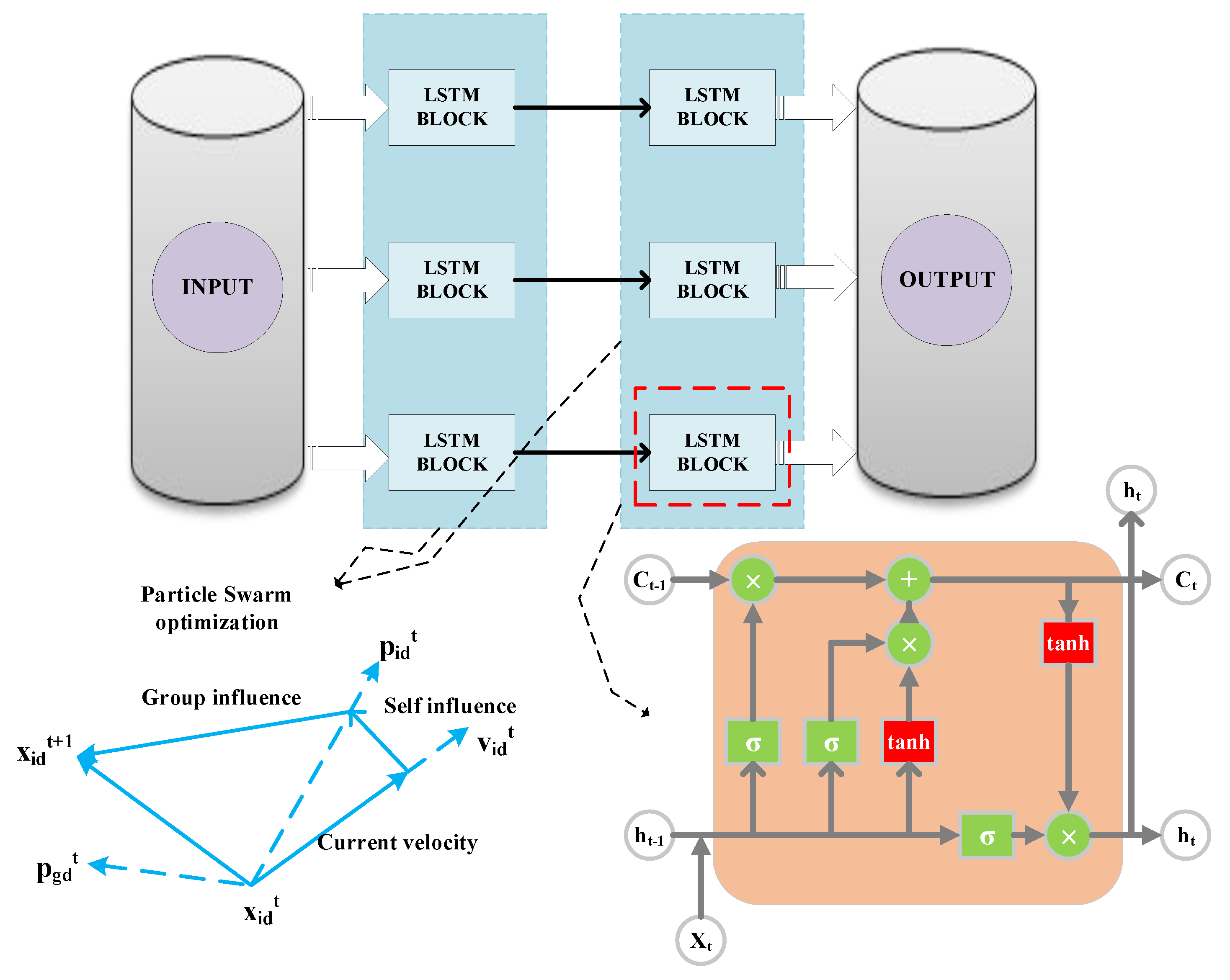
2.2. LSTM
LSTM has a long-term correlation learning ability, is improved compared with RNN, and is suitable for processing time series problems. LSTM adds cell states or memory cells on the basis of RNN to solve problems of traditional RNN [39]. It mainly includes the forget, input, and output gates [40]. The state vector discards useless memories through the forget gate, and the input gate adds the necessary information on the basis of the new input and the previous output. Finally, the output gate determines the new output of the corresponding unit. Figure 4 shows the single LSTM memory block.
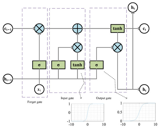
Figure 4.
Single LSTM block.
The process of updating the LSTM neurons was:
- (1)
- The output of and the current input were used as the inputs of the forgetting gate to obtain the output value of the forgetting gate based on Equation (1).where and were the parameters of the forgetting gate, was the activation function which typically used the sigmoid function, and the value range of ranged between 0 and 1. After the forgetting gate, the state vector of the LSTM was .
- (2)
- The output of and the current input were transformed nonlinearly as the input of the input gate to obtain a new state vector . controlled the amount of input through the input gate. The specific equations were Equations (2) and (3).where and were the parameters of the input gate, was the activation function, determined the acceptance of , and the value range of was between 0 and 1. After the input gate, the state vector of the LSTM was .
- (3)
- Update the state vector based on Equation (4).where the new state vector was obtained as the current state vector and the value range of was between 0 and 1.
- (4)
- The output of and the current input were used as inputs of the output gate to obtain the output of the output gate; the specific equation was Equation (5).where and were the parameters of the output gate, was the activation function which typically used the sigmoid function. The value range of was between 0 and 1.
- (5)
- Calculate the ultimate output value of the LSTM neurons based on Equation (6).
That is, interacted with the input gate after to obtain the final output of the LSTM. The value range of was between −1 and 1.
2.3. IPSO
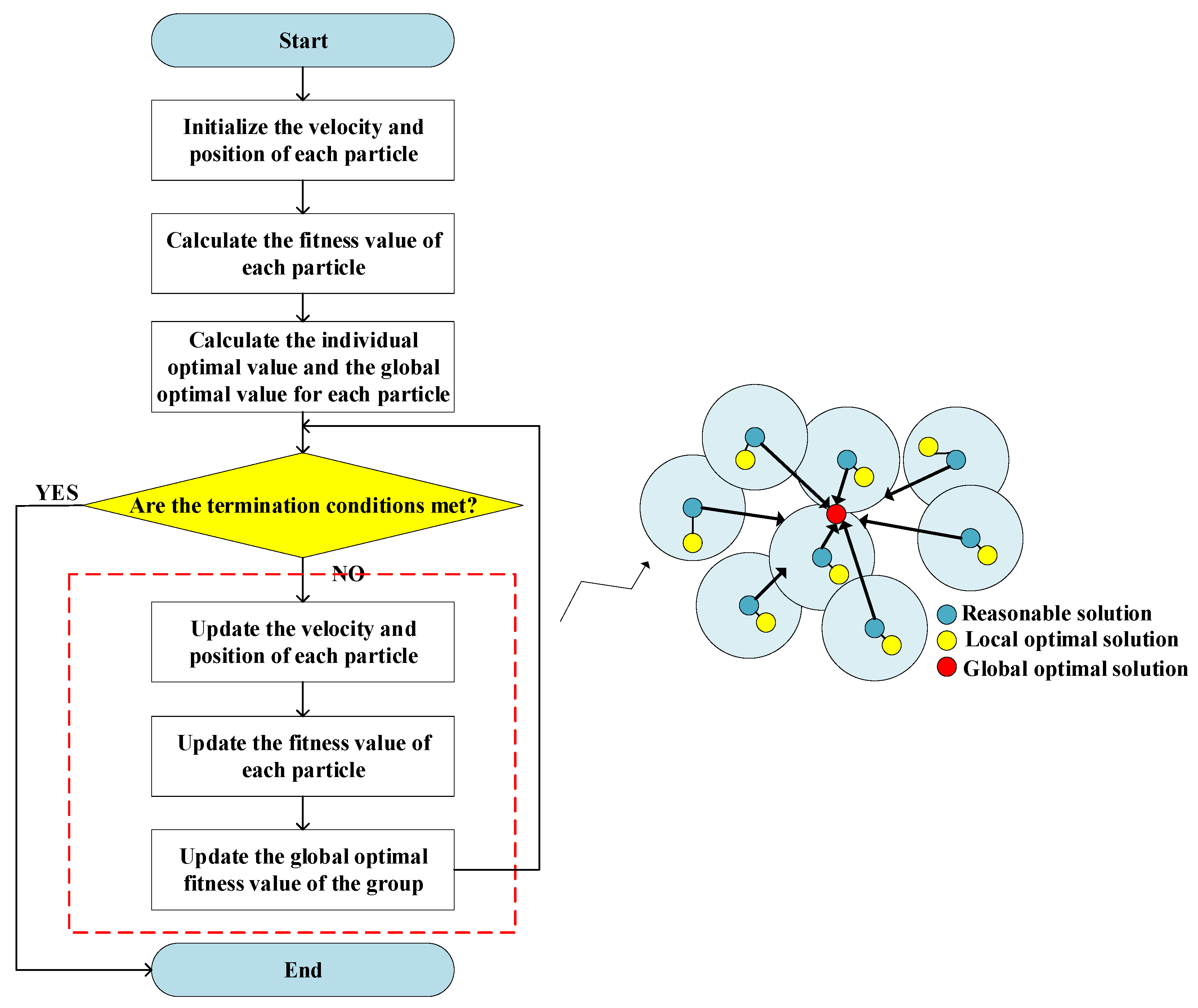
The PSO algorithm is used frequently to optimize complex numerical functions [41]. It originated from the study of the predatory behavior of bird flocks. In the PSO algorithm, there were several particles in the search space, wherein the algorithm attempted to optimize fitness functions. Every particle calculated its own fitness value based on its position in the search space. By combining information about its current position and its previous optimal position, the direction along which it would move was chosen. To obtain the final answer, these steps were repeated several times until the end condition was met [42,43,44]. Figure 5 shows the search process of the standard PSO.
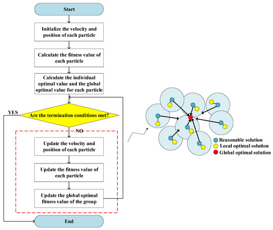
Figure 5.
Flow chart of standard particle swarm optimization algorithm.
In the case of the PSO algorithm, it was easy to fall into a local minimum value and fail to identify the global maximum value [45]. Based on various improvement experiences associated with the PSO, the learning factor and inertia weight were improved here.
- (1)
- Improvement in the inertia weight
When the inertia weight was large, the global search capability of the particle was enhanced and the local search capability was weakened. Conversely, when the inertia weight was small, the local search capability of the particle was enhanced and the global search capability was weakened. Proper adjustment of the inertia weight facilitated the rapid search of particles and improved the global search ability, but also facilitated local refinement and obtained a better global optimal solution in the shortest time. It was observed that selecting appropriate parameters was the key to the study and improved the capability of the PSO algorithm. The improvement equation was Equation (7).
where was the current number of iterations, the maximum number of iterations, and and were the maximum and minimum values of the inertia weights. Appropriate inertia weight played an important role in the search ability of IPSO. Combining previous research and real experimental results, we found that of 0.9 and of 0.3 were the most suitable for this model, which could achieve a balance between local search and global search.
- (2)
- Improvement of learning factors
Symbols and denoted the cognitive and social learning factors of the particles. Cognitive factors affected the local search performance and social factors affected the global search performance. Choosing appropriate learning factors was beneficial as they increased the convergence speed and avoided local extreme values. Equations (8) and (9) express the improvement formulas.
2.4. Model Evaluation Metrics
The model was validated with AQI index prediction experiments to evaluate the capability of the model and verify the effectiveness of the method. Training the model with excess training sets leads to the overfitting of the model, and training with insufficient training sets leads to the underfitting of the model. Therefore, selecting an appropriate data division method is vital for the accuracy of the model. Here, 8784 pieces of data were normalized, then 95% were selected as the training set and the remaining as the test set. Compared with BP, linear regression (LR), LSTM, EMD–LSTM, and EMD–IPSO–LSTM networks, the mean absolute error (), root-mean-square error (), mean absolute percentage error (), and R-square () were selected to evaluate the prediction performance of the model. Equations (10)–(13) express the relevant formulas.
where represented the predicted value, the true value, and the mean value. As the values of , , and became smaller, the model fitting effect was improved. Furthermore, as the value of came closer to 1, the model fitting effect was also improved.
3. Experiments
3.1. Data Sources and Preprocessing
This study selected 8784 pieces of historical monitoring information from three representative meteorological monitoring stations in Beijing from 1 January 2020 to 31 December 2020 as the experimental dataset. The dataset was obtained from the https://quotsoft.net/air/website accessed on 12 June 2021. Table 2 shows some of the data sets.
Table 2.
AQI data of Dongsi in 2020.
The collected data had to be preprocessed before being input in the model for training mainly owing to the following two aspects: first, there were missing values in the collected data which would influence the model predictive accuracy. Thus, before inputting the data into the model for training, the missing values needed to be filled. Given that the air pollutant concentration was influenced by the previous moment, the average of both previous values and the value of the next moment were used to deal with the missing values. Second, the different magnitudes made the prediction error larger. To reduce the large error where results were based on different types of data, the original data needed to be standardized, and the transformation function was Equation (14).
where was the mean of all data and the standard deviation of all data. This was by far the most common method of data standardization.
3.2. Predictive Modeling
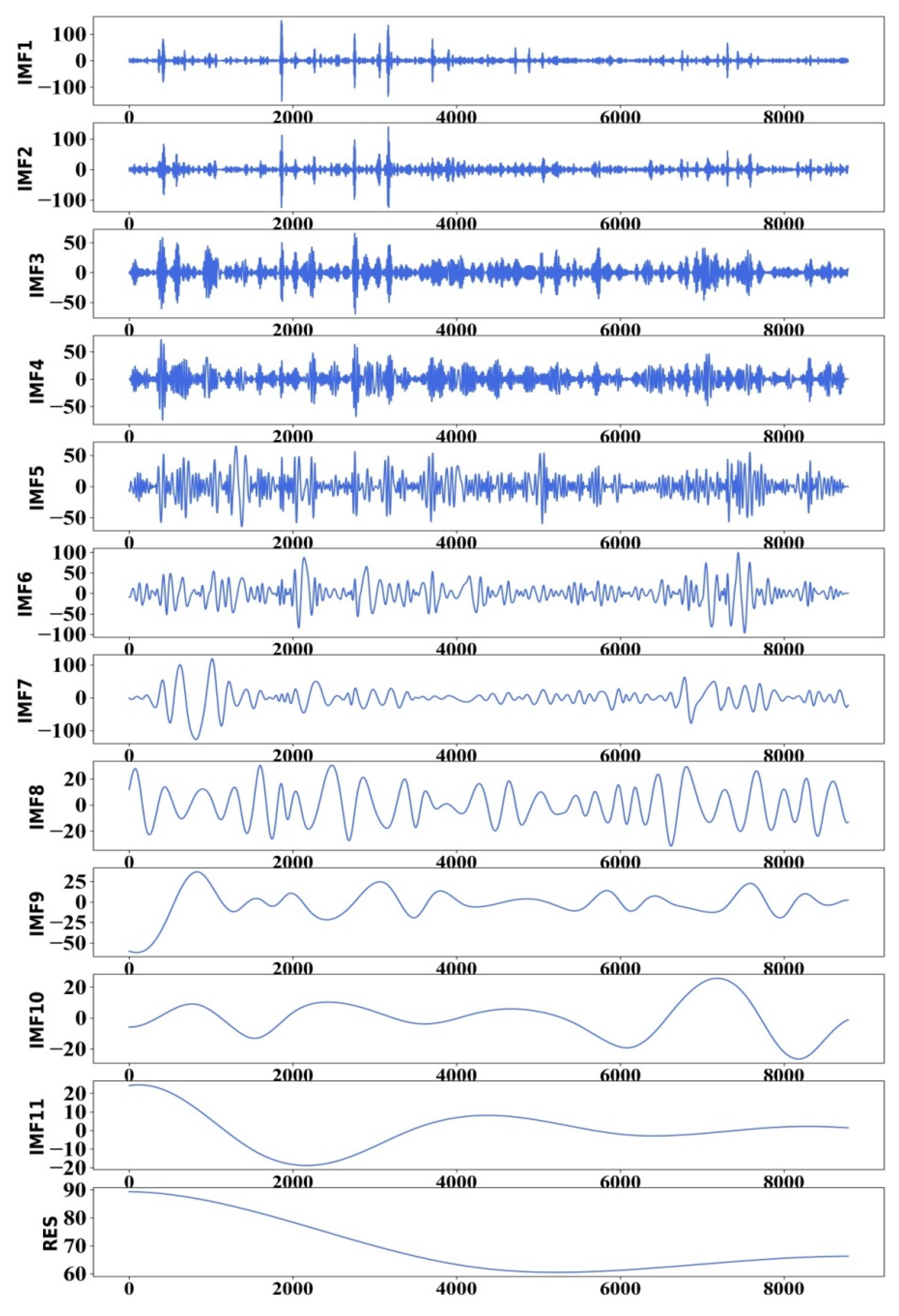
First, EMD was used to decompose the AQI sequence, and the AQI data were decomposed to the components of multiple IMF and to a residual component, which were respectively used as input variables of the EMD–LSTM model. Taking the Dongsi site as an example, the AQI values of the preceding 4 h period were used to predict the AQI value in the subsequent 1 h period. The AQI time series was decomposed in 11 IMF components and a RES component. Using the Dongsi station as an example, Figure 6 shows the EMD decomposition results.

Figure 6.
EMD decomposition results of Dongsi station.
It can be observed that the frequency of IMF1 is the highest; the frequencies of IMF2, IMF3, and IMF4 gradually decrease; and RES is the residual component. It is generally believed that the noise is mainly concentrated in the high-frequency IMF components and the low-frequency IMF components are less affected by the noise. However, deletion of the noise would reduce the prediction accuracy greatly. Hence, we retained all the IMF components.
Second, the EMD–LSTM prediction model was used to obtain the prediction value of each component. Third, the predictive results of each component were summarized to obtain the final prediction result.
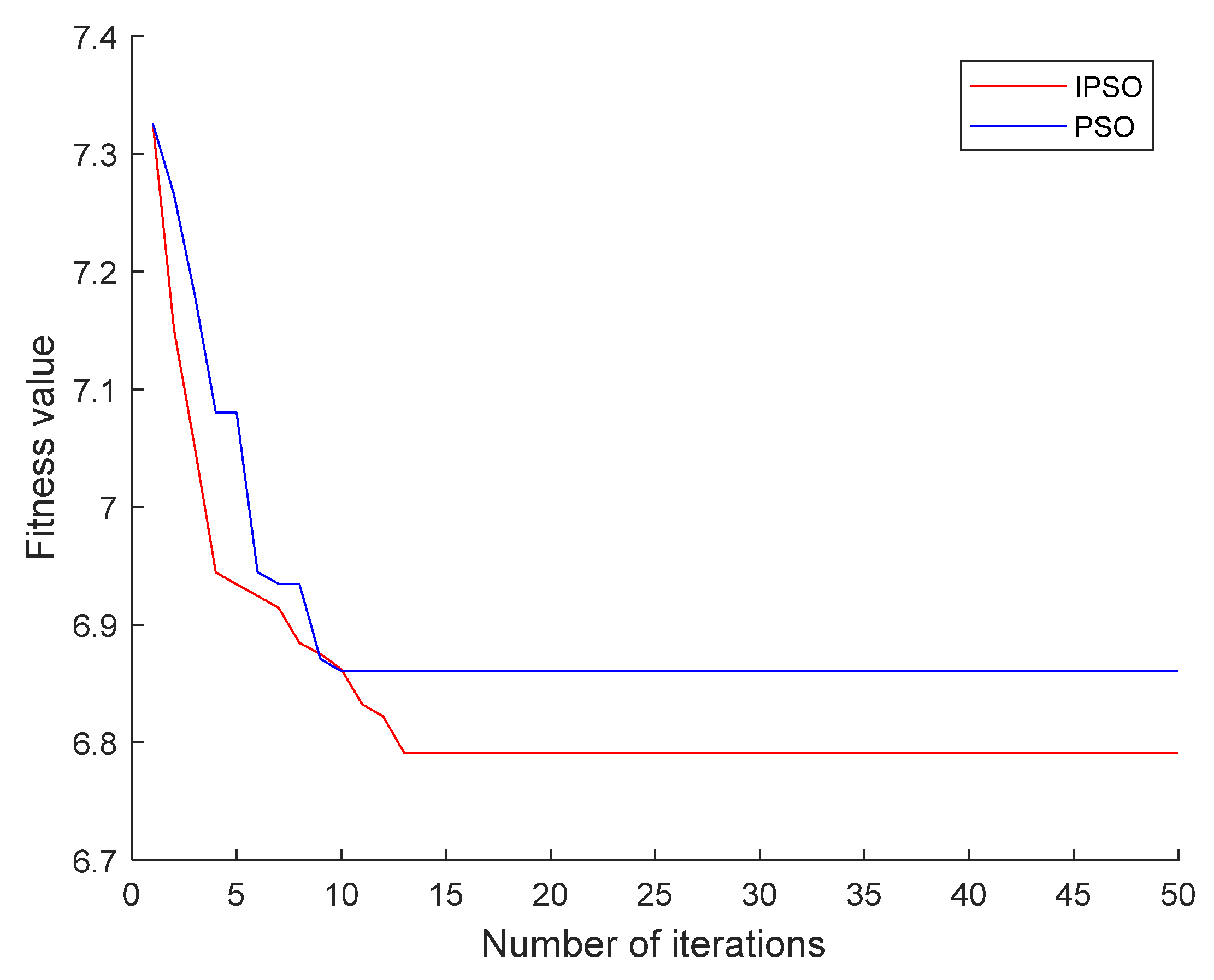
Because fewer neural network layers are difficult to fit complex data, more neural network layers lead to the complexity of the model. After repeated comparative experiments, we find that the two-layer neural network was sufficient to fit the training data, which can reduce the complexity of the model while ensuring the prediction accuracy. As Figure 7 shows, we chose a LSTM neural network with two hidden layers and used the PSO algorithm to find the optimal number of neurons L1 in the first layer and L2 in the second layer of the LSTM. To reach the global optimal value faster, an IPSO algorithm was designed to correct global optimal value here, and Figure 8 shows the algorithm comparison outcomes. When the results tend to converge, the fitness value of IPSO is smaller than that of PSO, indicating that the parameters found by IPSO are better than PSO and have higher prediction accuracy.

Figure 7.
Architecture of LSTM network.
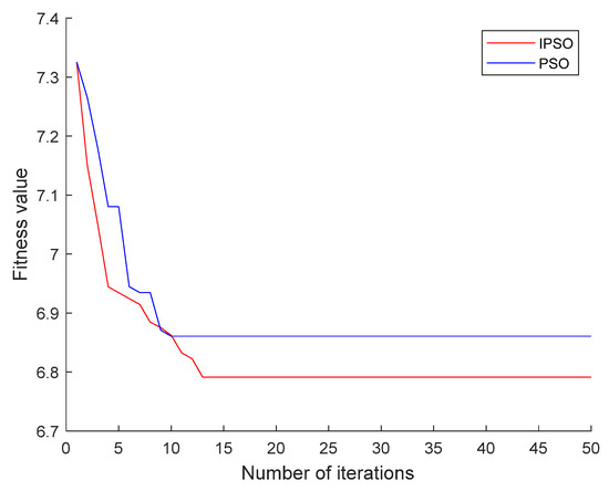
Figure 8.
Fitness curve.
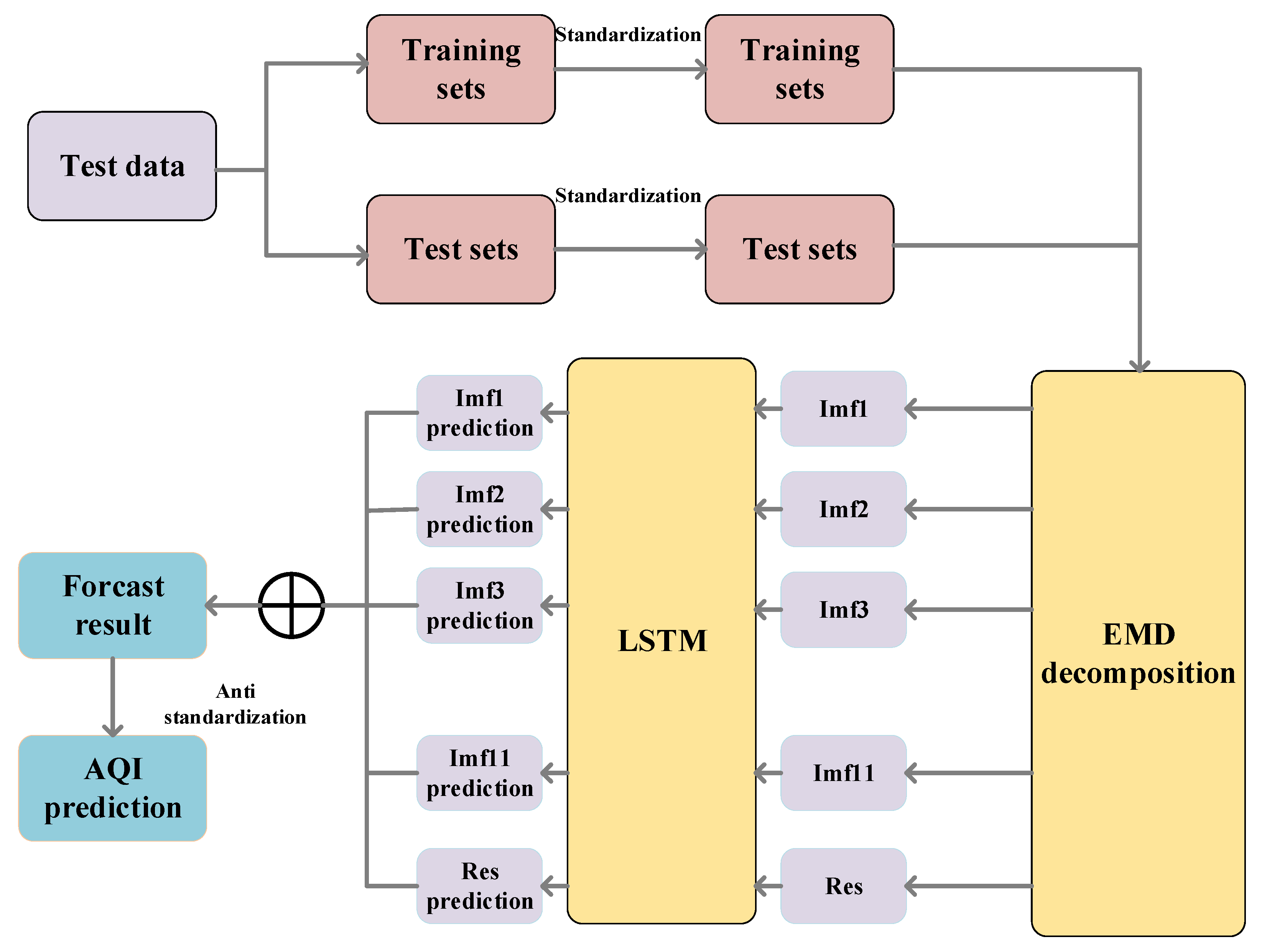
The output of each hidden layer of LSTM was used as the input of next layer, and the data were finally output through the fully connected layer. Figure 9 shows the architecture of the model. The specific steps were:
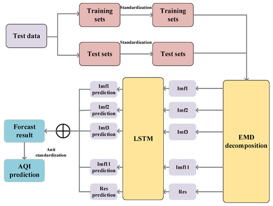
Figure 9.
Overall process of the model.
- (1)
- Normalize the AQI sequence and perform EMD decomposition to obtain multiple IMF and RES components. Then, 95% of the training set samples and 5% of the test set samples were selected and the raw data were transformed into supervised learning to predict the AQI for the future 1 h using data from the past 4 h.
- (2)
- After normalizing the original data, the normalized data were transformed into the data format required for LSTM, then the LSTM neural network was built. Due to the long training time of the LSTM neural network and the low efficiency of the multi-layer network, this experiment set up a two-layer LSTM which obtained better experimental results in the shortest time. Table 3 shows the main parameters of LSTM. Then, obtained components of IMF and the RES component were input into the LSTM neural network.
Table 3. Parameter description of LSTM.
- (3)
- Based on the multiple iterations of the training set, various parameters of the LSTM model network were trained. After the training set was trained, the prediction was performed on the test set and the components of the IMF prediction results were obtained.
- (4)
- Steps 2 and 3 were repeated to obtain the prediction results of the other components of the IMF and RES.
- (5)
- The predicted values of each IMF component and the remaining components were added, and inverse normalization was performed to obtain the final prediction results.
- (6)
- To initialize the IPSO parameters, we set the population size to 50 and the maximum number of iterations to 100. Taking the number of neurons in the two hidden layers of LSTM as the optimization goal, the optimization range is . MAE is selected as the objective function of the EMD–LSTM neural network, that is, the fitness of the IPSO algorithm function. Finally, through the IPSO algorithm, the optimal number of neurons in LSTM are L1 = 24 and L2 = 16. The number of hidden layer neurons obtained by IPSO is brought into EMD–LSTM, and we find that the model has higher prediction accuracy.
4. Results and Discussion
LSTM neural network was suitable for time series forecasting. However, although LSTM has achieved good results in handling time series problems, it did not achieve ideal results when applied to complex air quality data. Therefore, we summarize the main advantages and limitations of our proposed model according to the real datasets and use EMD combined with decomposition and reconstruction. For the decomposed components, the prediction accuracy is improved. The experimental results verify our hypothesis.
This paper chose the LSTM neural network as the core, which solved the long-term dependence problem of RNN. Simultaneously, EMD performed sequence decomposition according to the time scale characteristics of the sequence and had obvious advantages in processing nonlinear and nonstationary data. Finally, the particle swarm algorithm was proposed to improve the search speed. Considering the above reasons, we combined EMD and LSTM and used an IPSO to find the optimal solution for the number of neural units in LSTM.
To prove the effectiveness of the proposed model, we performed comparative experiments. The input characteristics of each model are seven-dimensional sequence data, and the output are one-dimensional data. We selected the data from the Dongsi monitoring station and used the five models of BP, LR, LSTM, EMD–LSTM and EMD–IPSO–LSTM to obtain the predicted values. Accordingly, the predicted values were compared with the true values. Then, the error was calculated to obtain the experimental result. Figure 10 shows the results of the Dongsi site. The results show that the EMD–IPSO–LSTM can better extract the potential characteristics of air quality data and has certain advantages in the prediction of AQI.
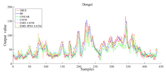
Figure 10.
Different model results of the Dongsi station.
Notably, in the comparative experiment, it is apparent that the prediction accuracy of LR is the worst, indicating that complex air quality data cannot be fitted using LR. Compared with other comparison models, the prediction performance of the proposed method is the best. In short, there are several reasons for this result. First, EMD decomposes the complex air quality data into multiple components; then, using only LSTM prediction, it can effectively improve the prediction accuracy. In addition, the improved PSO accurately extracts the best parameters of the model and improves the prediction performance of the LSTM, which further improves the accuracy of the proposed model.
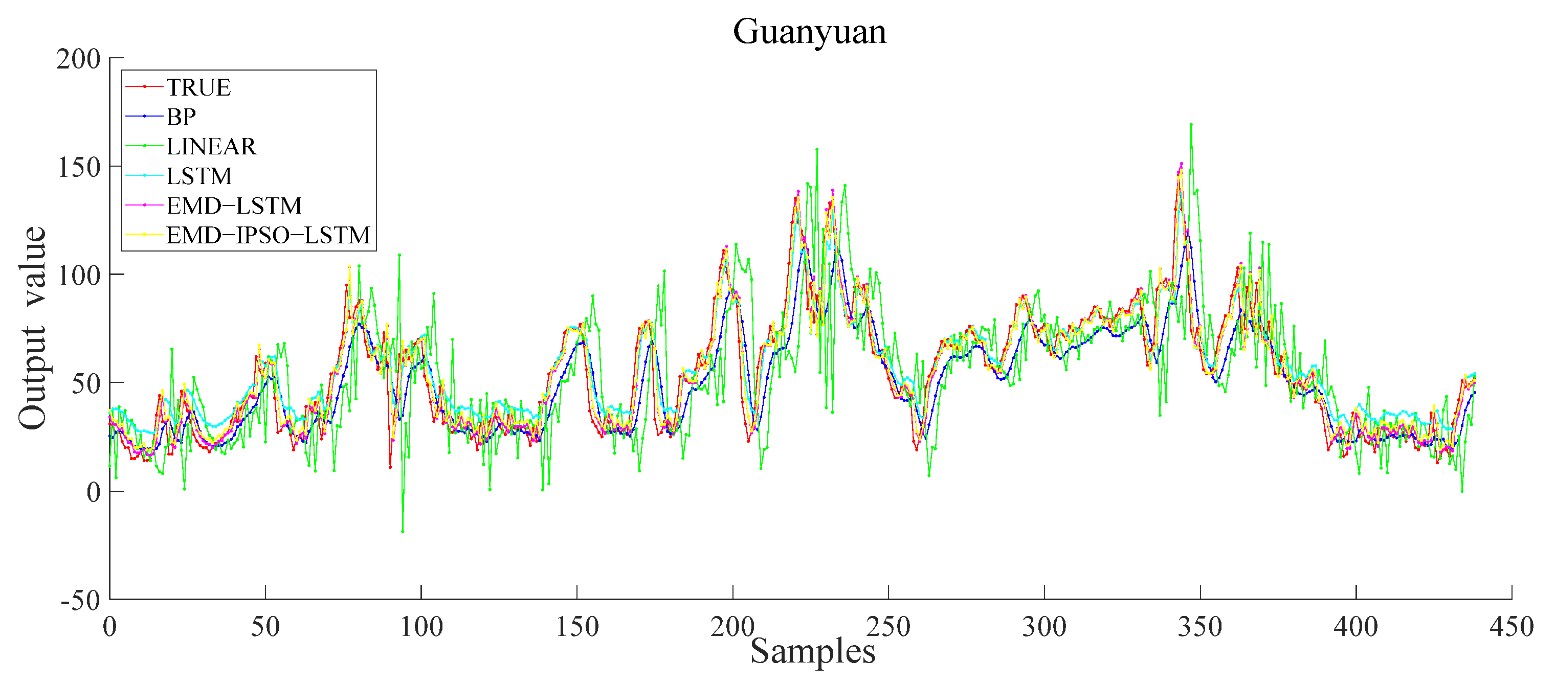
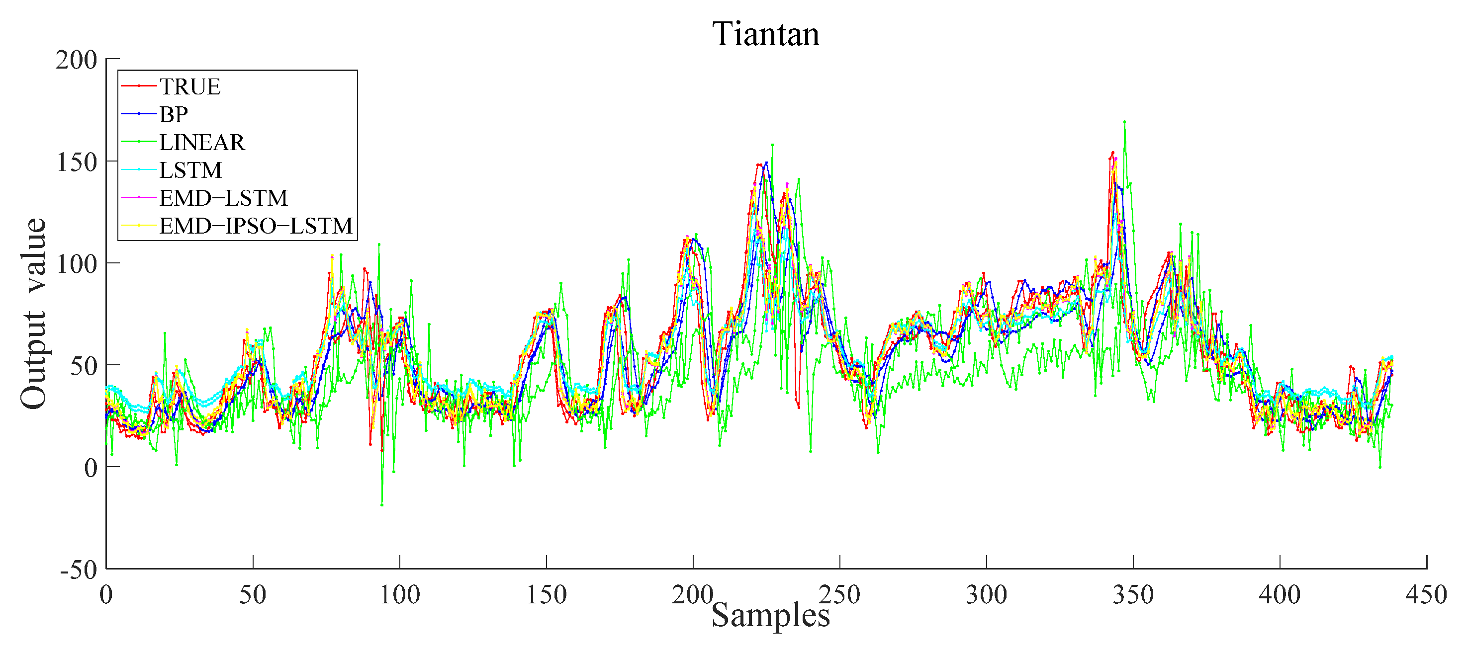
Next, to make the results of the model more convincing, we tested the stability of the model. We conducted the same comparative experiment on Guanyuan and Tiantan (see Figure 11 and Figure 12). The experimental results showed that the improved model had the highest prediction accuracy in the comparative experiment. The model was also suitable for Guanyuan and Tiantan, which further verified the model’s effectiveness.
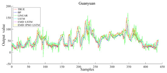
Figure 11.
Different model results of the Guanyuan station.
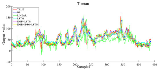
Figure 12.
Different model results of the Tiantan station.
To make the performance of the model more intuitive, Table 4 shows the evaluation indices of the BP, LR, LSTM, EMD–LSTM, and EMD–IPSO–LSTM models of the three sites of Dongsi, Guanyuan, and Tiantan. The errors and stability of the MAE, RMSE, MAPE, and R2 of the EMD–IPSO–LSTM model at the three stations were significantly improved, which provided more accurate air quality prediction accuracy than other models. The fluctuation trend of the predicted value was basically consistent with the actual value, which was used as a reference method for AQI prediction.
Table 4.
Air quality prediction performance index.
BP and LR are time series prediction models. The experimental results shows that the LSTM achieves a better fit of the data than the traditional ML model. Figure 10, Figure 11 and Figure 12 show that the fitting curve of the EMD–IPSO–LSTM model was smoother than those of the LSTM and the EMD–LSTM models (see Table 4). MAE, RMSE, and MAPE of the EMD–IPSO–LSTM model were all improved, and the R2 was closer to one. These findings proved that the long-term memory capability of the LSTM network optimized by the EMD decomposition and IPSO could have a better fitting effect on air-quality data. From an overall perspective, the combined EMD–IPSO–LSTM model was better in each index and had a better R2 fit.
The results showed that LSTM had long-term memory ability and high prediction accuracy. However, it was difficult to achieve the best performance with a single LSTM model for complex AQI data. After adding EMD, the prediction accuracy of the three stations was improved, which showed that EMD improved the prediction accuracy by decomposing complex time series data into time series with different frequencies. Similarly, in the comparative experiment of the three stations, it was seen that not selecting the appropriate parameters had a great impact on LSTM, worse than the BP neural network. Therefore, it was necessary to use a particle swarm optimization algorithm to find the optimal number of neural units of LSTM, which further improved the prediction accuracy of the model. Here, the EMD–IPSO–LSTM model was superior to other models in short-term air quality prediction and had practical application value.
Although this method accurately predicted AQI, the experimental data here was not sufficient due to experimental conditions. The results of this study can be further improved. Owing to the limitations of the air quality monitoring station data, we did not have information regarding the meteorological factors near the monitoring stations. Information regarding these factors would likely further improve the performance of our model and should be considered in future work. For example, temperature and wind would affect the diffusion of air pollutants. Future research should consider meteorological factors, vehicle emissions, and the interactions between different monitoring stations in the city, which would predict air quality more accurately. In addition, more advanced data interpolation technology could be used to replace cubic spline interpolation in EMD to reduce the error caused by fitting the envelope of each extreme point of the signal and improve the quality of signal decomposition.
5. Conclusions
Recently, air quality problems have seriously affected people’s health and daily life. Consequently, the prevention and control of air pollution has attracted public attention. Owing to the complex factors affecting air quality, AQI concentration series are complex and nonstationary. Therefore, accurate prediction of pollution is challenging. Traditional LSTM is a widely-used time series prediction method and an improvement of RNN. In addition, the LSTM can process data with long-term dependence and has a fast convergence speed. However, with the increase in complexity, it is difficult to provide accurate data to predict the AQI.
Here, a combined prediction model based on EMD–IPSO–LSTM was proposed. Based on the analysis of the AQI data of the three stations in Beijing in 2020, the following conclusions were drawn:
- (1)
- The decomposition of the data into multiple components of different frequencies through EMD decomposition and incorporating them into the LSTM model improved the accuracy of AQI prediction effectively.
- (2)
- The neural units in the hidden layer of LSTM were often determined themselves based on historical experience. Here, the PSO algorithm was selected for optimization and the optimal numbers of neurons in each layer were obtained.
- (3)
- Based on the slow convergence speed of the PSO, the problem of local optimization was easily countered; accordingly, a nonlinear decreasing inertia weight and a learning factor that changed with the inertia weight were proposed. These changes reduced the optimization time and led to a faster convergence toward the global optimum value.
- (4)
- Based on comparative experiments, it was observed that the EMD–IPSO–LSTM hybrid model proposed here had the best prediction performance, and the true and the predicted values had a high degree of fitting. These findings proved that the hybrid prediction method proposed here was effective for future AQI predictions. Therefore, this method has practical application value.
Author Contributions
Funding acquisition, Y.H.; Investigation, X.D. and Z.H.; Resources, Y.L.; Writing—original draft, J.Y. All authors have read and agreed to the published version of the manuscript.
Funding
This work was supported in part by the Project of the National Natural Science Foundation of China under Grant 61772451, in part by the Project of the University Science and Technology Research Youth Fund of Hebei Province under Grant QN2018073, and in part by the Project of the University Science and Technology Research Youth Fund of Hebei Province under Grant QN2019168.
Institutional Review Board Statement
Not applicable.
Informed Consent Statement
Not applicable.
Data Availability Statement
Not applicable.
Conflicts of Interest
The authors declare no conflict of interest.
References
- Carbajal-Hernández, J.J.; Sánchez-Fernández, L.P.; Carrasco-Ochoa, J.A. Assessment and prediction of air quality using fuzzy logic and autoregressive models. Atmos. Environ. 2012, 60, 37–50. [Google Scholar] [CrossRef]
- Yang, Z.S.; Wang, J. A new air quality monitoring and early warning system: Air quality assessment and air pollutant concentration prediction. Environ. Res. 2017, 158, 105–117. [Google Scholar] [CrossRef] [PubMed]
- He, H.D.; Li, M.; Wang, W.L. Prediction of PM2.5 concentration based on the similarity in air quality monitoring network. Build. Environ. 2018, 137, 11–17. [Google Scholar] [CrossRef]
- Zhai, W.X.; Cheng, C.Q. A long short-term memory approach to predicting air quality based on social media data. Atmos. Environ. 2020, 237, 117411. [Google Scholar] [CrossRef]
- Hu, F.P.; Guo, Y.M. Health impacts of air pollution in China. Front. Environ. Sci. Eng. 2021, 15, 74. [Google Scholar] [CrossRef]
- Cai, J.X.; Dai, X.; Hong, L. An Air Quality Prediction Model Based on a Noise Reduction Self-Coding Deep Network. Math. Probl. Eng. 2020, 2020, 3507197. [Google Scholar] [CrossRef]
- Yang, Z.C. DCT-based Least-Squares Predictive Model for Hourly AQI Fluctuation Forecasting. J. Environ. Inform. 2020, 36, 58–69. [Google Scholar] [CrossRef]
- Dimri, T.; Ahmad, S.; Sharif, M. Time series analysis of climate variables using seasonal ARIMA approach. J. Earth Syst. Sci. 2020, 129, 149. [Google Scholar] [CrossRef]
- Dun, M.; Xu, Z.C.; Chen, Y. Short-Term Air Quality Prediction Based on Fractional Grey Linear Regression and Support Vector Machine. Math. Probl. Eng. 2020, 2020, 8419501. [Google Scholar] [CrossRef]
- Ko, M.S.; Lee, K.; Kim, J.K. Deep Concatenated Residual Network with Bidirectional LSTM for One-Hour-Ahead Wind Power Forecasting. IEEE Trans. Sustain. Energy 2021, 12, 1321–1335. [Google Scholar] [CrossRef]
- Alotaibi, F.M.; Asghar, M.Z.; Ahmad, S. A Hybrid CNN-LSTM Model for Psychopathic Class Detection from Tweeter Users. Cogn. Comput. 2021, 13, 709–723. [Google Scholar] [CrossRef]
- Chen, Y.R.; Cui, S.H.; Chen, P.Y. An LSTM-based neural network method of particulate pollution forecast in China. Environ. Res. Lett. 2021, 16, 044006. [Google Scholar] [CrossRef]
- Choudhury, A.; Sarma, K.K. A CNN-LSTM based ensemble framework for in-air handwritten Assamese character recognition. Multimed. Tools Appl. 2021, 80, 35649–35684. [Google Scholar] [CrossRef]
- Ko, C.R.; Chang, H.T. LSTM-based sentiment analysis for stock price forecast. PeerJ Comput. Sci. 2021, 7, e408. [Google Scholar] [CrossRef]
- Liu, B.; Jin, Y.Q.; Li, C.Y. Analysis and prediction of air quality in Nanjing from autumn 2018 to summer 2019 using PCR-SVR-ARMA combined model. Sci. Rep. 2021, 11, 348. [Google Scholar] [CrossRef] [PubMed]
- Leong, W.C.; Kelani, R.O.; Ahmad, Z. Prediction of air pollution index (API) using support vector machine (SVM). J. Environ. Chem. Eng. 2020, 8, 103208. [Google Scholar] [CrossRef]
- Wang, P.; Zhang, H.; Qin, Z.D. A novel hybrid-Garch model based on ARIMA and SVM for PM2.5 concentrations forecasting. Atmos. Pollut. Res. 2017, 8, 850–860. [Google Scholar] [CrossRef]
- Du, B.; Liu, Y.R.; Atiatallah Abbas, I. Existence and asymptotic behavior results of periodic solution for discrete-time neutral-type neural networks. J. Frankl. Inst.-Eng. Appl. Math. 2016, 353, 448–461. [Google Scholar] [CrossRef]
- Liu, Y.R.; Liu, W.B.; Obaid, M.A. Exponential stability of Markovian jumping Cohen–Grossberg neural networks with mixed mode-dependent time-delays. Neurocomputing 2016, 177, 409–415. [Google Scholar] [CrossRef]
- Huang, A.L.; Wang, J. Wearable device in college track and field training application and motion image sensor recognition. J. Ambient Intell. Humaniz. Comput. 2021, 1–14. [Google Scholar] [CrossRef]
- Chinnappa, G.; Rajagopal, M.K. Residual attention network for deep face recognition using micro-expression image analysis. J. Ambient Intell. Humaniz. Comput. 2021, 1–14. [Google Scholar] [CrossRef]
- Chen, J.Y.; Zheng, H.B.; Xiong, H. FineFool: A novel DNN object contour attack on image recognition based on the attention perturbation adversarial technique. Comput. Secur. 2021, 104, 102220. [Google Scholar] [CrossRef]
- Sun, G.; Lin, J.J.; Yang, C. Stock Price Forecasting: An Echo State Network Approach. Comput. Syst. Sci. Eng. 2021, 36, 509–520. [Google Scholar] [CrossRef]
- Niu, H.L.; Xu, K.L.; Wang, W.Q. A hybrid stock price index forecasting model based on variational mode decomposition and LSTM network. Appl. Intell. 2020, 50, 4296–4309. [Google Scholar] [CrossRef]
- Carta, S.; Ferreira, A.; Podda, A.S. Multi-DQN: An ensemble of Deep Q-learning agents for stock market forecasting. Expert Syst. Appl. 2021, 164, 113820. [Google Scholar] [CrossRef]
- Lin, Y.H.; Ji, W.L.; He, H.W. Two-Stage Water Jet Landing Point Prediction Model for Intelligent Water Shooting Robot. Sensors 2021, 21, 2704. [Google Scholar] [CrossRef]
- Xie, J.; Chen, G.H.; Liu, S. Intelligent Badminton Training Robot in Athlete Injury Prevention Under Machine Learning. Front. Neurorobot. 2021, 15, 621196. [Google Scholar] [CrossRef]
- Ding, Y.H.; Hua, L.S.; Li, S.L. Research on computer vision enhancement in intelligent robot based on machine learning and deep learning. Neural Comput. Appl. 2021, 34, 2623–2635. [Google Scholar] [CrossRef]
- Seng, D.W.; Zhang, Q.Y.; Zhang, X.F. Spatiotemporal prediction of air quality based on LSTM neural network. Alex. Eng. J. 2021, 60, 2021–2032. [Google Scholar] [CrossRef]
- Qadeer, K.; Rehman, W.U.; Sheri, A.M. A Long Short-Term Memory (LSTM) Network for Hourly Estimation of PM2.5 Concentration in Two Cities of South Korea. Appl. Sci. 2020, 10, 3984. [Google Scholar] [CrossRef]
- Liu, D.R.; Hsu, Y.K.; Chen, H.Y. Air pollution prediction based on factory-aware attentional LSTM neural network. Computing 2020, 103, 75–98. [Google Scholar] [CrossRef]
- Arsov, M.; Zdravevski, E.; Lameski, P. Multi-Horizon Air Pollution Forecasting with Deep Neural Networks. Sensors 2021, 21, 1235. [Google Scholar] [CrossRef] [PubMed]
- Wang, J.Y.; Li, J.Z.; Wang, X.X. Air quality prediction using CT-LSTM. Neural Comput. Appl. 2020, 33, 4779–4792. [Google Scholar] [CrossRef]
- Cabaneros, S.M.; Calautit, J.K.; Hughes, B. Spatial estimation of outdoor NO2 levels in Central London using deep neural networks and a wavelet decomposition technique. Ecol. Model. 2020, 424, 109017. [Google Scholar] [CrossRef]
- Huang, G.Y.; Li, X.; Zhang, B. PM2.5 concentration forecasting at surface monitoring sites using GRU neural network based on empirical mode decomposition. Sci. Total Environ. 2021, 768, 144516. [Google Scholar] [CrossRef]
- Kong, X.Y.; Zhang, T. Improved Generalized Predictive Control for High-Speed Train Network Systems Based on EMD-AQPSO-LS-SVM Time Delay Prediction Model. Math. Probl. Eng. 2020, 2020, 6913579. [Google Scholar] [CrossRef]
- Luo, X.L.; Gan, W.J.; Wang, L.X. A Prediction Model of Structural Settlement Based on EMD-SVR-WNN. Adv. Civ. Eng. 2020, 2020, 8831965. [Google Scholar] [CrossRef]
- Shu, W.W.; Gao, Q. Forecasting Stock Price Based on Frequency Components by EMD and Neural Networks. IEEE Access 2020, 8, 206388–206395. [Google Scholar] [CrossRef]
- Sekertekin, A.; Bilgili, M.; Arslan, N. Short-term air temperature prediction by adaptive neuro-fuzzy inference system (ANFIS) and long short-term memory (LSTM) network. Meteorol. Atmos. Phys. 2021, 133, 943–959. [Google Scholar] [CrossRef]
- Wu, J.M.T.; Li, Z.C.; Herencsar, N. A graph-based CNN-LSTM stock price prediction algorithm with leading indicators. Multimed. Syst. 2021, 1–20. [Google Scholar] [CrossRef]
- Gundu, V.; Simon, S.P. PSO–LSTM for short term forecast of heterogeneous time series electricity price signals. J. Ambient Intell. Humaniz. Comput. 2020, 12, 2375–2385. [Google Scholar] [CrossRef]
- Kazemi, M.S.; Banihabib, M.E.; Soltani, J. A hybrid SVR-PSO model to predict concentration of sediment in typical and debris floods. Earth Sci. Inform. 2021, 14, 365–376. [Google Scholar] [CrossRef]
- Khari, M.; Armaghani, D.J.; Dehghanbanadaki, A. Prediction of Lateral Deflection of Small-Scale Piles Using Hybrid PSO–ANN Model. Arab. J. Sci. Eng. 2019, 45, 3499–3509. [Google Scholar] [CrossRef]
- Malik, A.; Tikhamarine, Y.; Sammen, S.S. Prediction of meteorological drought by using hybrid support vector regression optimized with HHO versus PSO algorithms. Environ. Sci. Pollut. Res. 2021, 28, 39139–39158. [Google Scholar] [CrossRef] [PubMed]
- Liu, H.B.; Dong, Y.J.; Wang, F.Z. Gas Outburst Prediction Model Using Improved Entropy Weight Grey Correlation Analysis and IPSO-LSSVM. Math. Probl. Eng. 2020, 2020, 8863425. [Google Scholar] [CrossRef]


Publisher’s Note: MDPI stays neutral with regard to jurisdictional claims in published maps and institutional affiliations. |
© 2022 by the authors. Licensee MDPI, Basel, Switzerland. This article is an open access article distributed under the terms and conditions of the Creative Commons Attribution (CC BY) license (https://creativecommons.org/licenses/by/4.0/).