A Dynamic Analysis for Mitigating Disaster Effects in Closed Loop Supply Chains

Abstract

The increased level of complexity in the case of Closed Loop Supply Chains (CLSCs) turns them into vulnerable systems under a disaster event. The latter calls for a methodological approach that allows a dynamic study under alternative policies in mitigating the disaster effects with a focus on creating sustainable CLSCs. For this reason, we provide a System Dynamics (SD)-based analysis for disaster events on the operation of CLSCs. By “disaster event”, we mean three different categories taking shape on the basis of duration. Furthermore, three different demand patterns emerging due to the disaster event are examined. We assume that the disaster event affects the manufacturer, and we examine the system response under different mitigation policies. For each demand pattern two different mitigation policies at the manufacturer level are examined by considering the total CLSC profit and demand backlog as measures of policy performance. For each combination, extensive simulation experimentation reveals sustainable policy recommendations under alternative settings regarding the reduction in the manufacturer’s production.

1. Introduction

The industrial world is increasingly exposed to risk as a result of major natural and man-made disasters, necessitating a rethinking of how industrial companies and communities recover [1]. Experience has shown that policies designed to operate within a given range of conditions are frequently confronted with unexpected challenges when they are used outside of that range due to an unexpected disaster event [2]. Makridakis et al. [3] proposed to distinguish between known–known, known–unknown, and unknown–unknown risks when handling uncertainty in a given situation. For a SC, disaster is a risk source of unknown–unknowns [4].

By “disaster”, we refer to extreme phenomena affecting the normal function of SCs to a great degree [5,6]. These phenomena can include natural disasters, such as typhoons [7,8] and earthquakes [9,10,11], or the spread of a pandemic as is the case with the COVID-19 disease [6,12,13]. They can be divided into three categories based on their duration: small-scale, medium-scale and large-scale. There are plenty real-world examples for each category: Earthquakes [9,10,11] are small-scale phenomena, such as the earthquake that hit Taiwan in 1999 and caused a two-week global semiconductor shortage because Taiwan was the world’s third largest provider of computer accessories when the phenomenon occurred [11].

Natural disasters, such as typhoons, are medium-scale phenomena [7,8]. Zhang Yi et al. [14] analyzed the economic loss of four selected ports in China due to typhoon-induced wind disasters from 2007 to 2017. The overall economic loss was calculated as the sum of reputational loss, loss to the shippers, loss to the carrier and loss to the ports and was approximately equal to $20 billion.

Finally, large-scale phenomena are outbreaks of diseases, epidemics and pandemics. For instance, disruptions caused by epidemics, such as the outbreak of mad cow disease in Europe (2001), which resulted in a shortage of leather goods, and the breakout of SARS in Asia (2003) that impacted information technology SCs, are large-scale phenomena [15]. Dixon et al. [16] mentioned that the trough of the economic downturn is expected to be around 19% at the end of the first quarter of 2020, with a 12% fall by the end of the second quarter. According to the CBO (2020), the Real GDP declined by 11% in the second quarter of this year, resulting in about 26 million fewer persons employed than in the fourth quarter of 2019.

A disaster effect may result in production disruptions with significant consequences on profitability. An important challenge is the identification of mitigation policies that should be implemented when production is disrupted due to disasters. In 2000, for example, Ericsson’s sole microchip source was the Phillips Electronics semiconductor factory in Albuquerque, New Mexico. Due to a fire caused by a lightning strike in 2000, this factory was destroyed, resulting in a $400 million loss for Ericsson [17].

On the contrary, Nokia, a competitor of Ericsson and a major customer of the same Philips Electronics plant, sensed this disruption following a multiple-supplier strategy and responsiveness and took immediate action by shifting its chip orders to other Philips factories and other Japanese and American suppliers. This quick response resulted in increasing Nokia’s handset market share from 27% to 30% [18]. According to estimates, 315 disasters occurred around the world in 2018, resulting in 11,804 deaths, 68.5 million people affected and $131.7 billion in economic damage [19].

Coordinated operations among supply chain actors and optimized emergency supply chain operations are critical to provide a speedy response to the presence of demand uncertainty, which remains one of the main challenges in disasters [20]. Ivanov and Dolgui [21] mentioned that the concerns that occurred particularly from the drastic increase or reduction in demand due to the COVID-19 pandemic cannot be handled within a narrow SC perspective but rather require a larger-scale analysis that goes beyond the current state-of-the-art in SC resilience.

In addition, Ivanov [22] presented the findings of a simulation study that opens up to some new research tendencies regarding the impact of COVID-19 on global SCs, specifically the consideration of different risk mitigation inventory levels as elements of pandemic plans. Umar and Wilson [23] adopted a multiple case study to examine the role of collaboration within food supply chains in two different South Asian regions in order to investigate how these capabilities influence the resilience of supply chains in rural communities that experience regular natural disasters.

Taking into consideration the relevant inventory policy suggestions by Ivanov [22] and the collaborative approach presented by Umar and Wilson [23], we provide an analysis based on System Dynamics (SD) that focuses on the development of effective policies in order to mitigate disaster effects for Closed-Loop Supply Chains (CLSCs).

In particular, we deal with a single manufacturer/multi-echelon CLSC with remanufacturing and recycling activities. The actors involved in the forward channel are the raw materials supplier, the parts producer, the manufacturer, the wholesaler and the retailer, while in the reverse channel it is the collector and the disassembly center that are involved. The reverse channel activities include the operations of disassembly, remanufacturing and recycling of used-product returns. Remanufacturing operations produce “as-good-as-new” parts for the manufacturer, while recycling operations supply the parts producer with recycled raw materials.

Moreover, we introduce dynamic feedback mechanisms, which control the rate of inflows and outflows for each echelon at both channels. We formulate a dynamic hypothesis about the effects of three (3) disaster scenarios on the manufacturer’s production, which are applied to each of the three categories of disaster events mentioned above (small-scale, medium-scale, large-scale).

We study the consequent economic impact on the manufacturer’s operations together with the side effects on the level of demand backlog. This study aims to fill the research gap by providing an SD model applicable to the disaster operations management in CLSCs. This dynamic analysis considers two different set of policies for mitigating the disaster effects. In the first case, the manufacturer follows alternative inventory management policies, regarding both the desired stock level and adjustment time in aligning the actual stock level with its desired value. In the second case, the manufacturer satisfies the wholesaler’s demand by contracting with a third-party producer who is not affected by the disaster event.

The above-mentioned policies were tested under alternative settings regarding the reduction in the manufacturer’s production due to the disaster event and also under the following demand patterns:

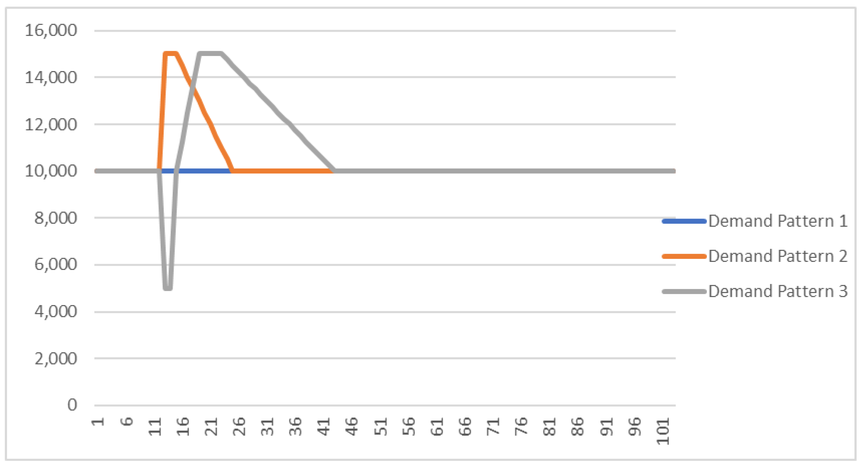
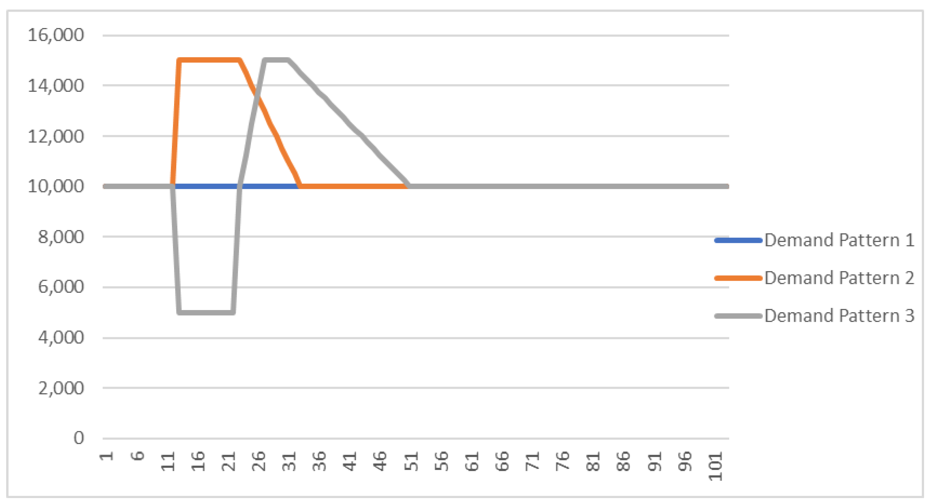
• Demand Pattern 1: Demand does not vary as a result of the phenomenon (for instance, food products during COVID-19 effect).
• Demand Pattern 2: Demand marks a sudden increase when disaster materializes. This increase is maintained for as long as the phenomenon last (disaster-period) and thereafter (post-disaster period) it returns to its pre-disaster level. An indicative example for this case is the sudden increase in demand for medical masks owing to the outbreak of COVID-19 [24].
• Demand Pattern 3: Demand marks a sudden decrease during the disaster period. During the post-disaster period, it increases to reach higher levels compared with pre-disaster conditions and after a certain amount of time, it returns to its pre-disaster level (for instance, the automotive industry during COVID-19 [24]).

In addition, we assume that the under study product is at the maturity stage of the product life cycle.

The rest of the paper is organized as follows: Section 2 provides a literature review of the basic elements of disaster management related to our study in order to identify the research gap and to justify the suitability of SD as an appropriate modeling approach. Section 3 presents a generic description of the CLSC under study and the formulation of effects due to a disaster event hitting the manufacturer. The mathematical representation of the SD model and mitigation policies are given in Section 4. Section 5 provides the settings of a numerical experimentation for each disaster scenario followed by a concluding discussion based on results gained by extensive simulation experimentation.

2. Literature Review

Τhere are many approaches that deal with different supply chain management issues, with a focus on sustainable CLSC. Wen-Hui et al. [25] introduced measures of the implementation of remanufacturing supply chain management in a CLSC. Hosseini-Motlagh et al. [26] studied the sustainability of a real pharmaceutical CLSC through effective collection interruption management. Ullah et al. [27] introduced mathematical models to reveal the best remanufacturing strategy and also reusable packaging capacity for single and multi-retailer CLSCs under stochastic demand and return rates.

Garai et al. [28] examined a CLSC for herbal medicines, while Garai and Sarkar [29] researched a CLSC for herbal medicines and biofuel by applying a minmax method based on a semi-autonomized multi-objective optimization algorithm from the economical point of view. By adopting a game-theoretical approach, Ma [30] examined different government subsidies for the management of CLSCs under demand disruption, in order to find the subsidies with the best economic and environmental benefit outputs. Sarkar et al. [31] proposed the conversion of a single food product supply chain into a two-stage supply chain in order to achieve zero waste through recycling. Although these contributions focus on sustainable CLSCs, the employed modelling and analysis approaches ignore issues related to disaster management.

In particular, disaster management in CLSCs has received increased attention over the last 15 years. It is remarkable that, although the topic is suitable for OR/MS research, the scientific community has not yet produced many articles dealing with operations management issues in large-scale disasters; interesting reviews of this field are provided in Altay and Green [5], Galindo and Batta [32] and Farahani et al. [33]. In addition, Borja et al. [34] mentioned that the literature on the dynamic behavior of CLSCs remains limited.

Complex adaptive systems theory [35,36,37], chaos theory [38,39,40], catastrophe theory [41], catastrophe-risk approaches [42], disaster preparedness [43], along with non-linear dynamic approaches [40,44,45], provide methods for the dynamic analysis and optimization of CLSCs under disaster effects. However, models based on these methods usually lead to more complex approaches and to more restrictions on the number of state variables and cost structure than they can handle.

Systems thinking may provide a systematic and structured approach to disaster management due to its ability to consider the systemic settings within a larger system. In addition, this approach may consider the interdependent nature of the system [46]. System-oriented and holistic approaches have been identified as important in modeling the complex, deeply uncertain and dynamic elements of disaster management [5,34,47].

The SD methodology introduced by Forrester [48] provides a more flexible and simple modeling and simulation framework for making decisions in dynamic and complicated industrial management situations [23,45]. It is an appropriate approach to study disaster operations problems in a CLSC context, mainly due to the following two reasons: (i) it has the ability to integrate soft factors into an operations analysis; (ii) it can deal with increased complexity caused by causal influences among different involved actors, non-linear behavior and time delays [46,49,50].

Additionally, the benefits of using SD models include: (i) allowing for the study and evaluation of alternative scenarios, making their impact on the system’s performance testable and (ii) being highly valued and well understood by managers, as they augment brainstorming and rely less on hard facts than other approaches [46]. This methodology provides an understanding of the changes occurring within a system by focusing on the interaction between physical flows, information flows, delays and policies that create the dynamics of the variables of interest.

Thereafter, the SD methodology searches for policies to improve system performance by considering the causal influences of relative decisions on the operational dynamics [51,52]. SD has been identified as promising for modeling complex and adaptive to nonlinear evolutionary change problems [47] and also as analysis tool to improve SC risk mitigation policies and recovery plans [53]. However, it is surprisingly underutilized in disaster operations management research [5,32,33] as shown in

Table 1. Methodological approaches in dealing with disaster management in CLSCs.

Approaches	Reference
Complex Adaptive Systems Theory	[35,36,37]
Chaos Theory	[38,39,40]
Catastrophe Theory	[41]
Catastrophe-Risk Approaches	[42]
Disaster Preparedness	[43]
System Dynamics	-
Non-Linear Dynamic Approaches	[40,44,45]

.

Some studies demonstrated SC dynamics as endogenous outcomes of feedback structures established under various dynamic hypotheses: Ozbayrak et al. [54] and Pierreval et al. [55] dealt with the dynamic analysis of manufacturing SCs and automotive industry, respectively; Keilhacker and Minner [56] applied an SD approach to examine the individual company’s reaction in the rare earth element (REEs) supply chain to China’s introduction of export restrictions; Lai et al. [57] studied the system dynamics in just-in-time logistics; Mikatia [58] examined the dependence of lead time on batch size in a manufacturing model; and Suryani et al. [59] studied capacity expansion decisions for innovative products with short lifecycles for the cement industry.

Other studies investigated the performance of SC systems under different operational disruption settings: Wilson [60] investigated the effect of transportation disruptions for the case of a five-echelon supply chain; Chen et al. [61] examined the effects of disruptions considering pipeline inventory control and vendor-managed inventory control; Ankit [62] studied the effects of SC between any two players in a multi-player SC system; and Aguila and ElMaraghy [63] proposed an SD model to study SC behavior in the face of interruptions.

The model may be used to predict the impact of potential interruptions on several critical performance indicators throughout the SC design and planning stage; Diaz et al. [64] proposed an SD model that analyzes the issue of housing recovery in the aftermath of a disaster, from both a demand and a supply standpoint; Bashiri et al. [65] investigated the sustainability risks in the Indonesia–UK coffee supply chain by using SD; and Zhang et al. [66] proposed an SD model to examine the effects of supply disruption, production disruption and sales disruption on the inventory, order accumulation rate and profit level of suppliers, manufacturers and retailers for a fixed outage time in a SC.

The contributions are limited when focusing on integrating aspects of SC and aspects of reverse logistics using SD [67]. Indeed, the formulation of dynamic strategic capacity planning policies [68,69], the examination of the bullwhip effect [70], the impact of environmental legislation on the long-term dynamic behavior of closed-loop remanufacturing networks [52] and the ecological and economic dimensions of sustainability in closed-loop recycling networks [71] are some of the few fields that have received special attention.

These models include either remanufacturing or recycling options of product reuse, while the integration of both remanufacturing and recycling into a closed-loop model for long-term evolutionary analysis and decision-making was introduced by Gu and Gao [72]. However, there is a gap in the SD literature in providing a dynamic approach for modeling and mitigation policy-making under disaster effects that considers a holistic picture of CLSC networks with remanufacturing and recycling options [73]. The purpose of this paper is to fill this gap by identifying effective policies in mitigating of disaster events.

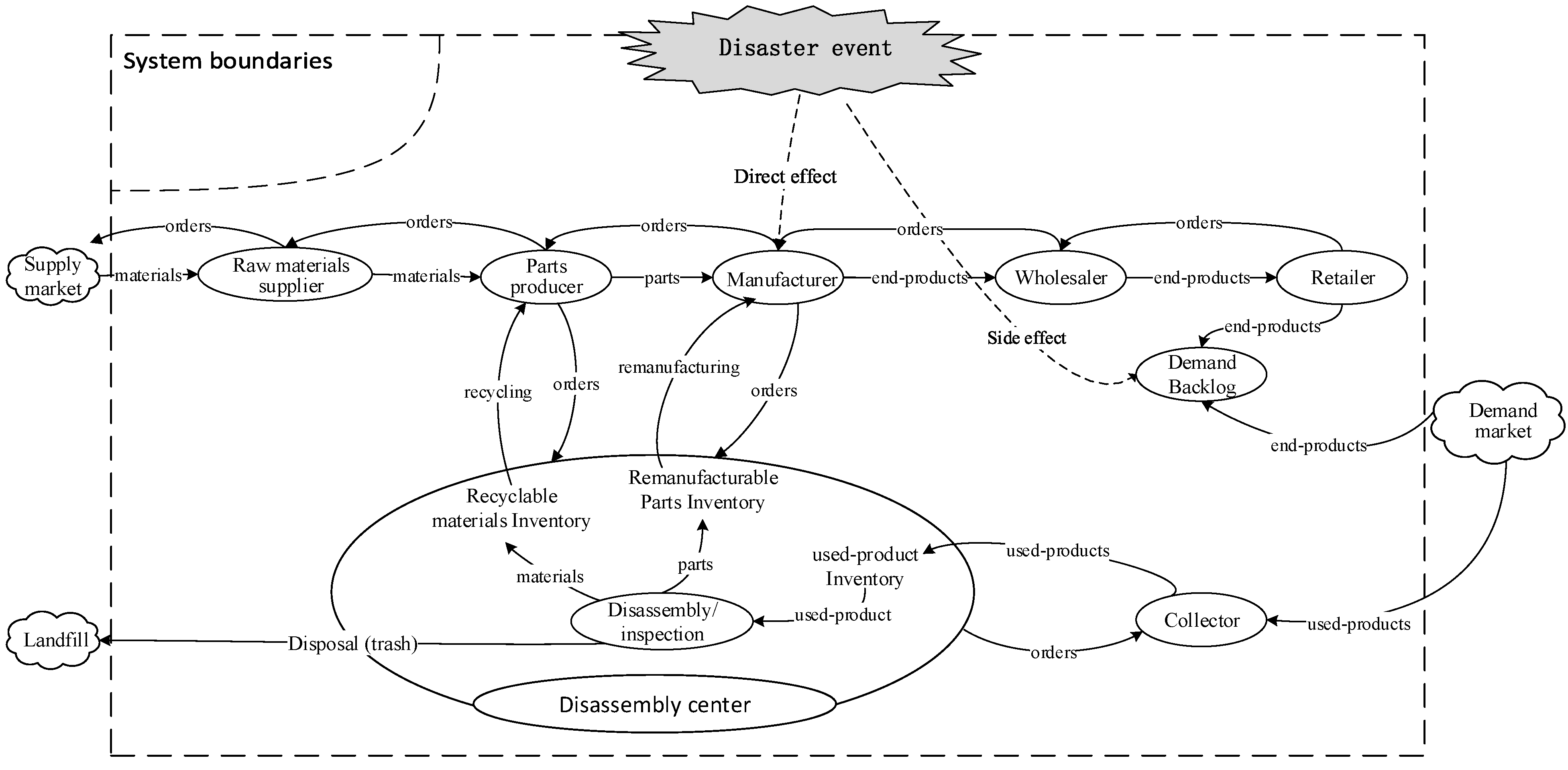
3. System and Problem Description

3.1. System Description

Figure 1 exhibits a very generic description of the CLSC under study. In particular, we deal with a single manufacturer/multi-echelon CLSC with remanufacturing and recycling activities. The forward supply chain comprises five echelons; Raw materials supplier, Parts producer, Manufacturer, Wholesaler and Retailer. The Raw materials supplier obtains materials from the Supply market. The Parts producer produces parts by using two inflows of materials; original raw materials by the Raw materials supplier and materials recovered by recycling.

Priority is given to supply with recycled materials. The Manufacturer produces end-products by assembling n = 1, 2, … N parts. The Manufacturer obtains these parts by using two inflows; original parts supplied by the Parts producer and parts obtained from a remanufacturing recovery process, which has priority over using original parts. The Wholesaler purchases end-products from the Manufacturer, while the Retailer purchases from the Wholesaler in order to satisfy the Demand Backlog. The latter is the level of all unsatisfied orders from Demand Market, which are backlogged in order to be satisfied in a subsequent time period.

The reverse channel includes the activities of collection (provided by the Collector), disassembly (provided by the Disassembly center), remanufacturing, recycling and Disposal. In particular, used-products are collected by the Collector for reuse and thereafter are transferred and sold to the Disassembly center. The re-manufacturability condition (quality) of parts obtained through the disassembly procedure is inspected to sort them in the remanufacturable stream. The condition of parts rejected for remanufacturing is inspected for recycling.

The parts accepted for recycling are sorted as recyclable materials, while those rejected are controllably disposed as trash (Disposal). The output of remanufacturing is “as-good-as-new parts” for the Manufacturer, while that of the recycling process is substitutes of virgin raw materials for the Parts producer. With regard to the buy/supply relationships among involved actors, we assume a single-supplier strategy in both channels, which means that a single Parts producer is the sole supplier for the Manufacturer, and the latter is the sole supplier for a single Wholesaler, etc.

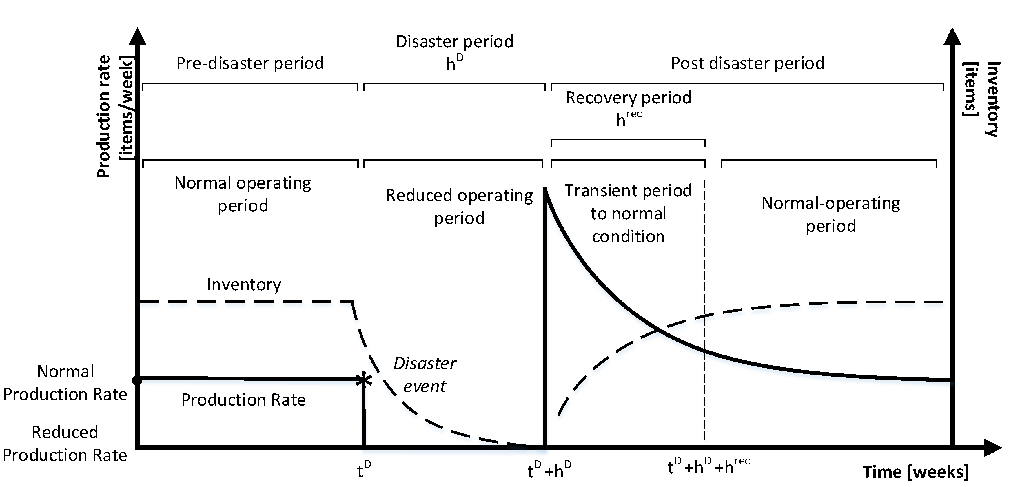
3.2. Problem Description

The main point of this paper is the examination of the dynamic behavior of a CLSC system under disaster effects hitting the manufacturer and the investigation of the efficiency of adopted alternative mitigation policies. This examination also takes into consideration the side effects of each mitigation policy on the demand backlog level.

The modeling of the disaster effect on the production rate of the manufacturer is shown in Figure 2, which illustrates a likelihood pattern for the production rate at the pre-disaster, disaster recovery and post-disaster time periods; t^D is the unknown time of occurrence of a disaster event, while h^D is the unknown duration of disaster event, and h^rec is the recovery period during which each mitigation policy is implemented by the manufacturer. This approach is based on the disaster resilience triangle concept originally introduced by Bruneau [74] and thereafter extended by Zobel and Khansa [75].

During the disaster event period (h^D), two options are considered regarding the disruptions of the manufacturer’s production rate due to the disaster effect: a 50% reduction of the production rate and a 20% reduction of the production rate.

4. The SD Model

Stocks and flows, along with feedback loops, are the two central characteristics of the SD theory. Stocks are the accumulations of the inflows and the outflows within the chain. SD uses a particular diagramming notation for stocks and flows [76]. Stocks are symbolized by rectangles; inflows are symbolized by pipes pointing into (adding to) the stock, and outflows are symbolized by pipes pointing out of (subtracting from) the stock. Stocks are defined by the stock equations as the time integrals of the net flows.

Flows are defined by the rate equations as the time functions of stocks and system parameters. In SD models, the stock and flow perspectives represent time as unfolding continuously; events can happen at any time, and change can occur continuously. The stock–flow diagram is translated into a system of differential equations, which is then solved via simulation, generally currently supported by high graphical simulation programs, such as PowerSim^®, Vensim^®, i-think^® and Stella^® [77].

The SD model’s full stock–flow diagram includes 30 stock variables, 58 rate variables, 151 auxiliary variables and over 45 balancing (negative) and reinforcing (positive) feedback loops. This section provides details regarding the mathematical modelling by keeping the analysis as generic as possible.

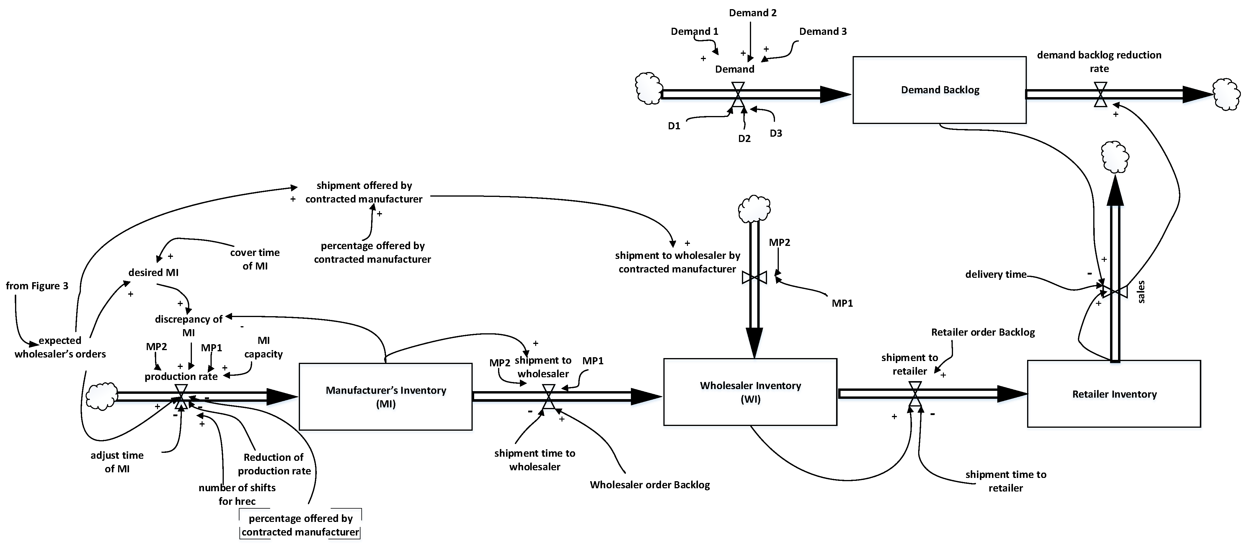
4.1. Generic Stock and Flow Structure

The generic stock–flow diagram is shown in Figure 3. The forward supply chain begins from the upper left corner. The Raw Materials Supplier’s Inventory (RMSI) is increased by the coming rate of new material and is decreased by the purchase rate of new material, which is the flow of virgin (new) materials to the parts producer. The demand of the parts producer for materials (total amount of the material) is satisfied with priority over recycled materials defining the recycling rate, while the unsatisfied part of demand is fulfilled by the raw materials supplier (purchase rate of new material).

The Parts Producer’s Inventory (PPI) is increased by the part production rate and is depleted by the purchase rate of new part. The manufacturer’s demand for parts (total amount of the part) is satisfied with priority over remanufactured parts, thus, defining the remanufacturing rate. The unsatisfied part of demand is fulfilled by supplies from the parts producer (purchase rate of new part). The production rate increases the Manufacturer’s Inventory (MI) in end-products, which is subsequently depleted by the shipment to wholesaler in order to satisfy as many of the wholesaler’s orders as possible. The Production rate is subject to the availability of inventory in parts; either recycled or new.

The shipments to the wholesaler take shipment time (shipment time to wholesaler) and deplete the wholesaler’s orders (wholesaler’s orders backlog). The shipment to the wholesaler increases the Wholesaler’s Inventory (WI). The Wholesaler’s Inventory is depleted by the shipment to retailer, which also takes shipment time (shipment time to retailer). The shipment to retailer depletes the retailer’s unfulfilled orders (retailer’s orders backlog) and increases the Retailer’s Inventory (RI). The latter is decreased by sales, which take delivery time to satisfy the demand for end-products (demand). All unsatisfied market demand is backlogged and satisfied in a subsequent time period (demand backlog). The same stands for orders placed by the retailer and directed to the wholesaler (retailer’s orders backlog), as well as for orders placed by the wholesaler and directed to the manufacturer (wholesaler’s orders backlog). Following a time delay (the usage period of a product), sales turn into used-products (coming rate 1).

The reverse channel starts with the collection activities. The stock of used-products at the collector (Collection Inventory (CI)) is increased by the expected collecting rate. The values of this rate are practically the forecasted values of the disassembly center’s demand for used-products. The Collection Inventory is depleted by supplies to the disassembly center (purchase rate), which also deplete the unsatisfied demand of the disassembly center (used-product should satisfy); the demand of the disassembly center for used-products is expressed by should satisfy rate of used-product, while the unsatisfied demand is backlogged and satisfied in a subsequent time period.

The purchase rate increases the Used-product inventory (UPI) at the disassembly center, which is depleted by the disassembly rate. The parts obtained through the disassembly operation (disassembly rate) are sorted into three streams. In particular, the output of the disassembly sorts the used-products (after inspection) with priority into remanufacturable parts. These parts (parts that can be remanufactured) increase the level of Remanufacturable Part Inventory. Parts rejected for remanufacturing are sorted as recyclable materials (material that can be recycled), which increase the level of Recyclable Material Inventory (RMI). Parts rejected for recycling are disposed as trash (remanent trash will be disposed). Finally, the remanufacturing rate delivers remanufactured parts to the manufacturer, while the recycling rate delivers recycled materials to the parts producer.

4.2. Mitigation Policies at the Manufacturer Level

Figure 4 represents the stock and flow structure of CLSC from production of the end-products to market demand satisfaction together with the implemented policies for mitigating the disaster effects. In particular, MP1 refers to the various mitigation policies regarding the serviceable inventory at the manufacturer level (Manufacturer’s Inventory (MI)). Their implementation is achieved through the alternation of the values for the adjusted time of MI and the cover time of MI parameters (base stock expressed in time units), which refer to the time for achieving the desired value for MI and to the level of the desired value for MI (Desired MI see Equation (14)), respectively.

In the case of MP2, the manufacturer enters into a contract with a third-party manufacturer who will fulfill a percentage (percentage offered by the contracted manufacturer) of the expected wholesaler’s orders placed by the wholesaler only during the disaster period and recovery period. Parameters MP1 and MP2 shown in Figure 4 take dual values (0/1), activating (MP_i = 1) or deactivating (MP_i = 0) the corresponding MP_i. The sets of control parameters that fully describe MP1 and MP2 are the following:

• MP1: [MP_1, cover time of MI, cover time of MI due to event, adjust time of MI, adjust time of MI due to event, h^rec].
• MP2: [MP₂, cover time of MI, cover time of MI due to event, adjust time of MI, adjust time of MI due to event percentage offered by contracted manufacturer, h^rec].

The mathematical representation for MP₁ and MP₂ is given by the following equations; where equations are differentiated, the values of parameters MP_i are given to indicate the active mechanism.

4.3. Stock Equations

$$\mathrm{MI}\left(t\right)=\mathrm{MI}\left(t=0\right)+{{\displaystyle \int }}_0^t\left[\mathrm{production} \mathrm{rate}\left(t\right)- \mathrm{shipment} \mathrm{to} \mathrm{wholesaler}\left(t\right)\right] \mathrm{d}t$$

(1)

$$\mathrm{WI}\left(t\right)=\mathrm{WI}\left(t=0\right)+{{\displaystyle \int }}_0^t\left[\begin{array}{c}\mathrm{shipment} \mathrm{to} \mathrm{wholesaler}\left(t\right)+\mathrm{shipment} \mathrm{to} \mathrm{wholesaler} \mathrm{by} \mathrm{the} \mathrm{contracted} \mathrm{manufacturer}\left(t\right)\\ - \mathrm{shipment} \mathrm{to} \mathrm{retailer}\left(t\right)\end{array}\right] \mathrm{d}t$$

(2)

$$\mathrm{Retailer} \mathrm{Inventory}\left(t\right)=\mathrm{Retailer} \mathrm{inventory}\left(t=0\right)+{{\displaystyle \int }}_0^t\left[\mathrm{shipment} \mathrm{to} \mathrm{retailer}\left(t\right)- \mathrm{sales}\left(t\right)\right] \mathrm{d}t$$

(3)

$$\mathrm{Demand} \mathrm{Backlog}\left(t\right)=\mathrm{Demand} \mathrm{Backlog}\left(t=0\right)+{{\displaystyle \int }}_0^t\left[\mathrm{Demand}\left(t\right)- \mathrm{demand} \mathrm{backlog} \mathrm{reduction} \mathrm{rate}\left(t\right)\right] \mathrm{d}t$$

(4)

4.4. Flow Equation

$$\begin{gathered} \begin{array}{l}\mathrm{production} \mathrm{rate}(t)=\\ \\ \{\begin{array}{c}\min \left(\begin{array}{c}\mathrm{M}\mathrm{I} \mathrm{c}\mathrm{a}\mathrm{p}\mathrm{a}\mathrm{c}\mathrm{i}\mathrm{t}\mathrm{y},\\ \mathrm{e}\mathrm{x}\mathrm{p}\mathrm{e}\mathrm{c}\mathrm{t}\mathrm{e}\mathrm{d} \mathrm{w}\mathrm{h}\mathrm{o}\mathrm{l}\mathrm{e}\mathrm{s}\mathrm{a}\mathrm{l}\mathrm{e}\mathrm{r}’\mathrm{s} \mathrm{o}\mathrm{r}\mathrm{d}\mathrm{e}\mathrm{r}\mathrm{s} \left(t\right)+\frac{\mathrm{discrepancy}\mathrm{of}\mathrm{MI}\left(t\right)}{\mathrm{adjusted}\mathrm{time}\mathrm{of}\mathrm{MI}}\end{array}\right) \mathrm{f}\mathrm{o}\mathrm{r} t\langle t^D\mathrm{a}\mathrm{n}\mathrm{d} t\rangle t^D+h^D+h^{rec}\\ \mathrm{m}\mathrm{i}\mathrm{n}\left[\begin{array}{c}\mathrm{M}\mathrm{I}\mathrm{capacity}\ast \mathrm{reduction}\mathrm{of}\mathrm{the}\mathrm{production}\mathrm{rate},\left(100-\mathrm{percentage}\mathrm{offerd}\mathrm{by}\mathrm{the}\mathrm{contracted}\mathrm{manufacturer}\left(t\right)\right)\ast \\ \ast \left(\mathrm{expected}\mathrm{wholesaler}’\mathrm{s}\mathrm{orders}\left(t\right)+\frac{\mathrm{discrepancy}\mathrm{of}\mathrm{MI}\left(t\right)}{\mathrm{adjusted}\mathrm{time}\mathrm{of}\mathrm{MI}}\right)\end{array}\right]\mathrm{f}\mathrm{o}\mathrm{r} t^D\le t \le t^D+h^D+h^{\mathrm{rec}}\end{array}\end{array} \end{gathered}$$

(5)

$$\begin{array}{c}\mathrm{shipment} \mathrm{to} \mathrm{wholesaler}\left(t\right)\\ =\{\begin{array}{c}\left(\frac{\min (\mathrm{MI}\left(t\right),\mathrm{wholesaler}\text{’}\mathrm{s}\mathrm{orders}\mathrm{backlog}\left(t\right))}{\mathrm{shipment}\mathrm{time}\mathrm{to}\mathrm{wholesaler}}\right) \mathrm{for} M{P}_1=1\\ \{\begin{array}{c}\frac{\min \left(\mathrm{MI}\left(t\right),\mathrm{wholesaler}\text{’}\mathrm{s}\mathrm{orders}\mathrm{backlog}\left(t\right)\right)}{\mathrm{shipment}\mathrm{time}\mathrm{to}\mathrm{wholesaler}} \mathrm{for}t<t^D \mathrm{and} {t\text{>}t}^D{+h}^D+h^{rec}\\ \mathrm{for} M{P}_2=1\\ \frac{\min \left(\mathrm{MI}\left(t\right),\mathrm{wholesaler}\text{’}\mathrm{s}\mathrm{orders}\mathrm{backlog}\left(t\right)\right)}{\mathrm{shipment}\mathrm{time}\mathrm{to}\mathrm{wholesaler}}-\mathrm{shipment}\mathrm{to}\mathrm{wholesaler}\mathrm{by}\mathrm{contracted}\mathrm{manufacturer}\left(t\right) {\mathrm{for}t}^D\le t\le t^D{+h}^D+h^{rec}\end{array}\end{array}\end{array}$$

(6)

$$\begin{array}{l}\mathrm{shipment} \mathrm{to} \mathrm{wholesaler} \mathrm{by} \mathrm{contracted} \mathrm{manufacturer} \left(t\right)\\ =\{\begin{array}{c}0 \mathrm{for} M{P}_1=1\\ \{\begin{array}{c}0 \mathrm{for} t<t^D \mathrm{and} { t>t}^D{+h}^D+h^{rec}\\ \hspace{1em}\hspace{1em}\hspace{1em}\hspace{1em}\hspace{1em}\hspace{1em}\hspace{1em}\hspace{1em}\hspace{1em}\hspace{1em}\hspace{1em}\hspace{1em}\hspace{1em}\hspace{1em}\hspace{1em}\hspace{1em}\hspace{1em}\hspace{1em}\hspace{1em}\hspace{1em}\hspace{1em}\mathrm{for} M{P}_2=1\\ {\mathrm{expected} \mathrm{wholesalers} \mathrm{orders}\ast \mathrm{percentage} \mathrm{offered} \mathrm{by} \mathrm{contracted} \mathrm{manufacturer} \mathrm{for} t}^D\le t\le t^D{+h}^D+h^{rec}\end{array}\end{array}\end{array}$$

(7)

$$\mathrm{shipment} \mathrm{to} \mathrm{retailer}\left(t\right)=\frac{\min (\mathrm{WI}\left(t\right), \mathrm{retailer}’\mathrm{s} \mathrm{orders} \mathrm{backlog}\left(t\right))}{\mathrm{shipment} \mathrm{time} \mathrm{to} \mathrm{retailer}}$$

(8)

$$\mathrm{sales}\left(t\right)=\frac{\min (\mathrm{Retailer} \mathrm{Inventory}\left(t\right), \mathrm{Demand} \mathrm{Backlog}\left(t\right))}{\mathrm{delivery} \mathrm{time}}$$

(9)

4.5. Auxiliary Equations

$$\mathrm{percentage} \mathrm{offered} \mathrm{by} \mathrm{contracted} \mathrm{manufacturer}\left(t\right)=\{\begin{array}{c}0 \mathrm{f}\mathrm{o}\mathrm{r} M{P}_1=1 \\ \\ \mathrm{p}\mathrm{e}\mathrm{r}\mathrm{c}\mathrm{e}\mathrm{n}\mathrm{t}\mathrm{a}\mathrm{g}\mathrm{e} \mathrm{o}\mathrm{f}\mathrm{f}\mathrm{e}\mathrm{r}\mathrm{e}\mathrm{d} \mathrm{b}\mathrm{y} \mathrm{t}\mathrm{h}\mathrm{e} \mathrm{c}\mathrm{o}\mathrm{n}\mathrm{t}\mathrm{r}\mathrm{a}\mathrm{c}\mathrm{t}\mathrm{e}\mathrm{d} \mathrm{m}\mathrm{a}\mathrm{n}\mathrm{u}\mathrm{f}\mathrm{a}\mathrm{c}\mathrm{t}\mathrm{u}\mathrm{r}\mathrm{e}\mathrm{r}\left(t\right) \mathrm{f}\mathrm{o}\mathrm{r} M{P}_2=1\end{array} [\%]$$

(10)

$$\mathrm{discrepancy} \mathrm{of} \mathrm{MI}\left(t\right)=\mathrm{desired} \mathrm{MI}\left(t\right)- \mathrm{MI}\left(t\right)$$

(11)

desired MI(t) = cover time of MI ∗ expected wholesaler’s orders(t)

(12)

$$\mathrm{adjust} \mathrm{time} \mathrm{of} \mathrm{MI} =\{\begin{array}{ll}\mathrm{initial} \mathrm{adjust} \mathrm{time} \mathrm{of} \mathrm{MI}& \mathrm{for} t<t^D{ \mathrm{and} t>t}^D{+h}^D\\ \mathrm{adjust} \mathrm{time} \mathrm{of} \mathrm{MI} \mathrm{due} \mathrm{to} M{P}_i& \mathrm{for} t^D\le t\le t^D{+h}^D+h^{rec} \end{array}$$

(13)

$$\mathrm{cover} \mathrm{time} \mathrm{of} \mathrm{MI} =\{\begin{array}{ll}\mathrm{initial} \mathrm{cover} \mathrm{time} \mathrm{of} \mathrm{MI}& \mathrm{for} t<t^D{ \mathrm{and} t>t}^D{+h}^D\\ \mathrm{cover} \mathrm{time} \mathrm{of} \mathrm{MI} \mathrm{due} \mathrm{to} M{P}_i& \mathrm{for} t^D\le t\le t^D{+h}^D+h^{rec}\end{array}$$

(14)

expected wholesalers’ orders = DELAYMTR (wholesaler orders; Tm; 1; wholesaler orders)

(15)

Equations (1)–(4) represent the stock equations for MI, WI, Retailer Inventory and Demand Backlog in end-products. The inflow to MI is the production rate (see Equation (5)), and the outflow from MI is the shipment to wholesaler, which is defined by Equation (6). At the same time, shipment to wholesaler constitutes the inflow to WI. The second inflow to WI is the shipment to wholesaler by contracted manufacturer (see Equation (7)). The outflow from WI (shipment to retailer) is defined by Equation (8). The inflow to Retailer Inventory is the same with the outflow of WI (shipment to retailer), while the outflow from Retailer Inventory is sales, which is defined by Equation (9). The inflow to Demand Backlog (demand) is determined under alternative demand patterns, while the outflow from Demand Backlog (demand backlog reduction rate) is equal to sales.

In Equation (5), the production rate is defined for the normal operating period, the disaster period and the recovery period h^rec as the combination of the expected wholesaler’s orders with an adjustment that brings the MI in line with its desired value (desired MI). The production rate is subject to the availability of actual stock in parts. The percentage offered by contracted manufacturer in Equation (5) is defined by Equation (10) under MP₂, while the expected wholesaler’s orders is a forecasted value for wholesaler’s orders (see Figure 3 and Equation (15)) calculated from a first-order exponential smoothing. The adjustment of MI is based on a proportional rule that controls the discrepancy (discrepancy of MI) between desired MI and actual MI (Equation (11)).

The adjustment time (adjust time of MI) represents how quickly the manufacturer decides to close the gap between the desired and the actual inventory level. It expresses the incorporated mitigation policies during the disaster period and the recovery period h^rec. Especially during the disaster period and during the recovery period h^rec, the value of adjust time of MI is decreased so as for the system to be able to respond to the changes caused by the disaster event (see Equation (13)). Cover time of MI (see Equation (14)) is the base stock expressed in time units.

4.6. Profit Equations

Profit equations are provided through profit per period (Profit) and Total Profit as the sum of Profit (profit per simulation time-step) over the simulation horizon. The Profit is captured by monetary flows created by physical flows per period (Profit calculation in Figure 3).

$$\mathrm{Profit}\left(t\right)=\mathrm{Sales}\left(t\right)\ast \mathrm{Price}–\mathrm{Operational} \mathrm{Cos}\mathrm{ts}\left(t\right) [€/\mathrm{tu}]$$

(16)

$$\mathrm{Total} \mathrm{Profit}\left(t\right)=\mathrm{Total} \mathrm{Profit}\left(t=0\right)+{{\displaystyle \int }}_0^t\left[ \mathrm{Sales}\left(t\right)\ast \mathrm{price} -\mathrm{Operational} \mathrm{Cos}\mathrm{ts}\left(t\right)\right]\mathrm{d}t [€]$$

(17)

Sales and Price refer to market demand. Operational Costs include: (i) the production, inventory holding and transportation costs in the forward channel, i.e., the sum of operational costs for the raw materials supplier (RMScost), the parts producer (PPcost), the manufacturer (Mcost), the wholesaler (Wcost) and the retailer (Rcost); (ii) the collection, disassembly, remanufacturing, recycling, transportation, holding and disposal costs in the reverse channel, i.e., the sum of operational costs for the collector, the disassembly center, the remanufacturer and the recycler; and (iii) the cost of supplies by a contracted third-party manufacturer in the case of MP₂. The detailed income/cost equations are based on standard calculations.

5. Numerical Experimentation and Discussion

By utilizing the SD model, we conducted a simulation experimentation in order to examine the system response to the effect of a disaster event. Our target was to search for sustainable mitigation policies that allow the manufacturer to return as soon as possible to normal condition operations through transitional dynamics. During this experiment, we considered the total CLSC profit and demand backlog as measures of policy performance. Throughout investigation, the output results are presented as ratios to the corresponding values obtained by the simulation run of the basic scenario (namely, Profit index, Total profit index, Demand Backlog index). The basic scenario (BS) refers to a CLSC operation under normal conditions (disaster-free model).

5.1. Validation of the SD Model

Structure and behavior validity are the basic criteria for the validation of an SD model. These are detected following certain procedures and tests suggested by the SD literature [46,78,79].

The above-mentioned tests were conducted as follows: First, we checked the dimensional consistency of the model. Then, we conducted extreme condition tests to assess whether or not the model behaved realistically even under extreme situations. For example, we verified that if no used products were collected, only raw materials were used for production, or that, in the absence of demand, production ceased. Integration error tests were subsequently conducted. The model employs the Euler integration method with an integrating time-step equal to 1 week. The results of the tests indicated no integrating errors. Structural validation tests were executed, which confirmed the sensitivity of the model structure to specific parameters.

Due to the absence of real data and published research for a point-by-point match between model behavior and real behavior, the behavior validation of the SD model was tested by comparing the simulation results obtained by running the disaster-free model with those provided by the literature. In particular, Figure 5 shows that the accumulated level of inventory at the manufacturer (MI, see Equation (1) and Figure 4) exhibited similar dynamic behavior compared to that provided by Yadav et al. [80]. The comparative study of simulation results with those given by Gu and Gao [72], resulted in similar dynamic behavior regarding the crucial rate variables, namely, the production rate (see Equation (5)), part production rate and disassembly rate (see Section 4.1 and Figure 3).

5.2. Settings

The SD model was executed for a simulation horizon of 24 months with time-step equal to 1 week. The Demand at normal operation conditions for end-products followed a normal distribution function [Demand ~N (10,000 items/week, 1,000 items/week]. We assumed that normal operation conditions belongs to the maturity stage of product life cycle, while the CLSC refers to products that are included in the group of furnishings and household equipment (major household appliances whether electric or not and small electric household appliances). The time of disaster occurrence was equal to t^D = 12 [week], while the duration of the disaster period (h^D) was examined under three sets of value: 2 weeks (small-scale); 6 weeks (medium-scale); 10 weeks (large-scale). The alternative demand patterns (Demand Pattern 1, Demand Pattern 2 and Demand Pattern 3) due to the disaster event (see explanation in Section 1) are given in Figure 6, Figure 7 and Figure 8.

The sale price of end-product is equal to 200 €/end-product.

The alternative mitigation policies are expressed by the following sets of control parameters:

• MP1: [MP_1, cover time of MI, cover time of MI due to event, adjust time of MI, adjust time of MI due to event, h^rec].
• MP2: [MP₂, cover time of MI, cover time of MI due to event, time of MI, adjust time of MI due to event, percentage offered by contracted manufacturer, h^rec].

Finally, the settings for the basic scenario are as follows:

• BS: [Demand ~N(10,000 items/week, 1000 items/week, stock management: cover time of MI = 4 weeks; adjust time of MI = 6 weeks].

5.3. Recommendations for Mitigating Disaster Effects

We concentrate on the efficiency of two mitigation policies for the manufacturer in responding to the demand market. Specifically, we examine the dynamic response of the system for three categories of disaster event, three sets of demand patterns and under two possible mitigation policies in combination with: (i) four sets of values for the cover time of MI due to event (2, 4, 6 and 8 weeks); (ii) five sets of value for the adjustadjusted time of MI due to event (1, 2, 3, 4 and 6 weeks); (iii) two sets of value for the reduction of production rate (20% and 50%); and (iv) three sets of value for the h^rec (4, 8 and 12 weeks).

All possible combinations (3 × 3 × 2 × 4 × 5 × 2 × 3 = 2160) represent a broad area of response scenarios for mitigating the effects of disaster event. For each combination, 20 repetitive simulation runs were conducted to test for alternative generators of random numbers (used in definition of Demand), thus, giving a total of 2160 × 20 = 43,200 runs. In each run, the values of stock variables and of smoothing functions were first initialized by considering an initialization horizon of 260 weeks in order to capture the system’s behavior outside its transient region.

Thereafter, a simulation horizon of 24 months, starting at t = 0 and using time-step equal to 1 week, represents the real-time experimentation for each combination. Throughout investigation, the CLSC profitability (profit per week (Profit)—see Equation (15), Total profit—see Equation (16) and Demand Backlog level—see Equation (4), (as the mean values of 20 repetitive runs) are considered as the output of the relative combinations for each category of disaster event and each demand pattern. The output results are presented as ratios to the corresponding values obtained by the simulation run of the basic scenario (i.e., Profit index, Total profit index and Demand Backlog index). The basic scenario (BS) refers to a CLSC operation under normal conditions (disaster-free model).

5.3.1. Profitability of the CLSC System

Table 2. Best/worst mitigation policies according to the Total Profit Index.

hD (Weeks)	Reduction of Production Rate	Demand Pattern	Best/Worst Cases	MP *	hrec (Weeks)	Adjust Time due to Event (Weeks)	Cover Time due to Event (Weeks)	$$\begin{gathered} \mathbf{Total} \mathbf{Profit} \mathbf{Index} \\ \left[\frac{\mathbf{T}\mathbf{o}\mathbf{t}\mathbf{a}\mathbf{l} \mathbf{p}\mathbf{r}\mathbf{o}\mathbf{f}\mathbf{i}\mathbf{t}{ }_{\mathbf{t}}}{\mathbf{T}\mathbf{o}\mathbf{t}\mathbf{a}\mathbf{l} \mathbf{p}\mathbf{r}\mathbf{o}\mathbf{f}\mathbf{i}\mathbf{t}{ }_{\mathbf{t}}^{\left(\mathbf{B}\mathbf{S}\right)}}\ast 100\right] \end{gathered}$$
								Lower	Upper	Equilibrium State
2	0%	1	Basic Scenario (BS)					100	100	100
	20%	1	Best	MP2	12	1	2	100	106.58	100.88
			Worst	MP2	12	2	8	80.41	99.93	95.90
	20%	2	Best	MP2	12	4	2	99.81	142.83	105.60
			Worst	MP2	12	2	8	95.67	119.84	103.60
	20%	3	Best	MP2	12	2	2	82.59	160.12	137.00
			Worst	ΜP1	12	4	8	73.29	154.10	134.00
	50%	1	Best	MP1	12	2	2	100	109.66	100
			Worst	MP2	12	4	8	85.73	99.30	96.60
	50%	2	Best	MP1	12	4	2	99.87	145.95	106.80
			Worst	MP1	12	3	6	96.61	130.04	105.45
	50%	3	Best	MP1	12	3	2	85.49	162.30	137.40
			Worst	MP1	8	6	8	76.92	148.91	123.90
6	20%	1	Best	MP2	12	2	2	98.93	108.97	99.00
			Worst	MP2	12	2	8	82.13	97.99	94.58
	20%	2	Best	MP2	12	2	2	99.26	156.45	108.20
			Worst	MP1	12	4	8	95.90	132.55	107.50
	20%	3	Best	MP2	12	2	2	65.08	151.73	133.86
			Worst	MP1	12	4	8	45.07	145.35	131.60
	50%	1	Best	MP1	8	4	2	100.33	114.48	100.53
			Worst	MP2	12	1	8	91.84	99.17	97.79
	50%	2	Best	MP1	12	3	2	101.13	163.40	109.82
			Worst	MP2	8	3	6	97.82	147.99	107.97
	50%	3	Best	MP1	12	4	2	67.64	155.12	135.10
			Worst	MP1	12	3	8	53.80	147.33	132.97
10	20%	1	Best	MP2	8	6	2	98.11	110.12	98.15
			Worst	MP2	8	3	8	83.04	98.43	95.35
	20%	2	Best	MP2	12	1	2	100.13	166.10	111.00
			Worst	MP1	12	4	8	96.17	143.76	110.90
	20%	3	Best	MP1	12	3	2	50.33	144.16	131.52
			Worst	MP2	12	2	8	30.72	135.70	125.90
	50%	1	Best	MP1	12	4	2	99.94	119.43	100.90
			Worst	MP1	4	6	8	93.41	102.90	99.13
	50%	2	Best	MP1	8	2	2	100.88	178.86	113.40
			Worst	MP1	8	4	8	97.66	158.60	112.70
	50%	3	Best	MP1	12	4	2	58.92	148.35	133.80
			Worst	MP1	12	2	8	42.75	137.77	127.70

* MP1: mitigation policies regarding the serviceable inventory at the manufacturer level (see Section 4.2); MP2: a contract with a third-party manufacturer who will fulfill a percentage of expected wholesaler’s orders (see Section 4.2).

displays the best and worst mitigation policies in each set of values for disaster event under each combination of reduction of production rate and demand pattern. Note that the results refer to the period from the appearance of the disaster event to the end of the simulation period. The lower/upper limits of the Total profit index express the detected minimum/maximum values. Depending on the combination, we found that the best policy recommendations are either MP1 or MP2 combined with specific values of cover time of MI due to event, adjust time of MI due to event and h^rec.

Taking all the above into consideration, we observe that, from an economic perspective, it is preferable to preserve a low security stock (defined by cover time of MI due to event) upon materialization of the disaster event, throughout its duration and during the recovery period (h^rec). In addition, it is preferable for the duration of h^rec to be long (8 or 12 weeks). For example, in the case of h^D = 6 weeks and reduction of production rate = 20%, from Table 2, we found that the best policy recommendations were: MP2, h^rec = 12 weeks, adjust time due to event = 2 weeks and cover time due to the event = 2 weeks for all demand patterns.

It is necessary to combine this safety stock with the time parameters regarding system control at MI level, because—as it appears from the results—a wrong combination may have undesirable consequences on the Total Profit. Another very important observation is that cooperation with a third party (MP2) is recommended in cases where the duration of the disaster event (h^D) or the reduction of production rate fluctuate among small values. In the opposite cases, MP1 with the appropriate adjustments to the rest of the parameters is preferable. Finally, we observe that, if the best mitigation policies are implemented, the system returns to the same or an even better condition compared with the one in the pre-disaster period.

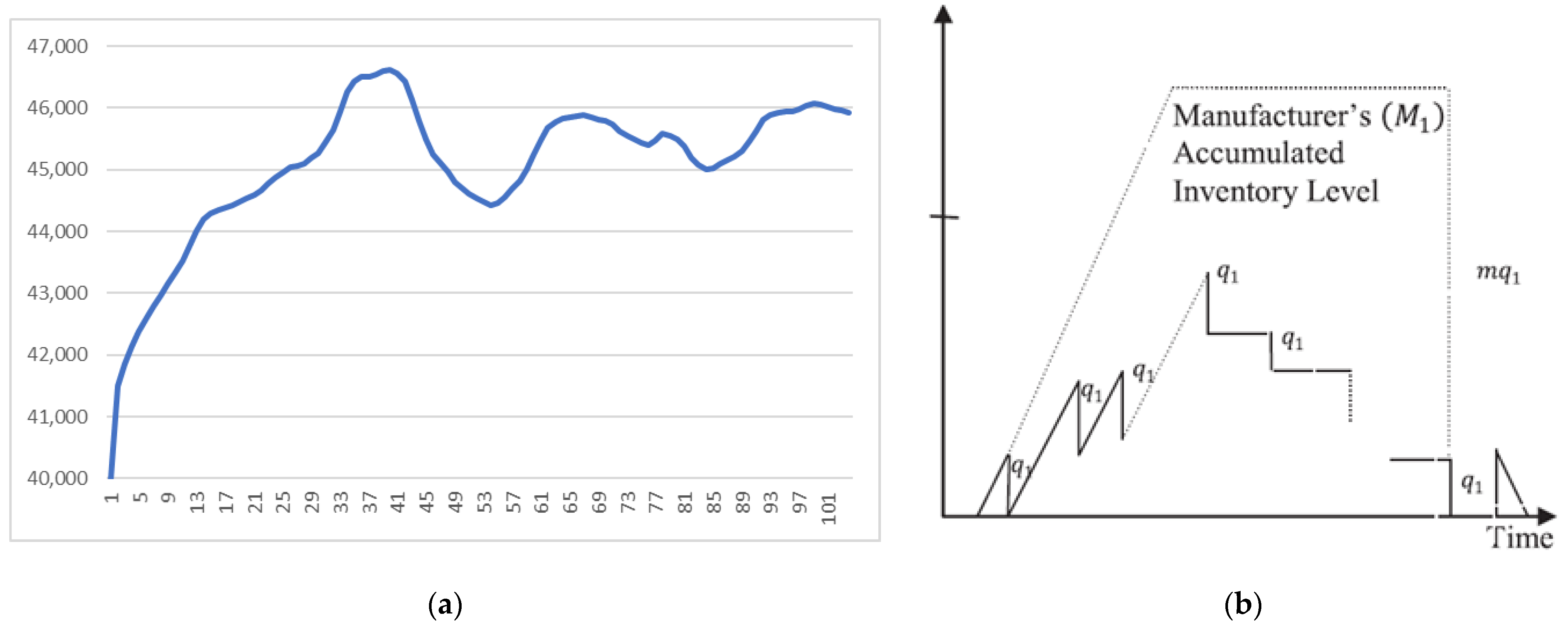
5.3.2. Demand Backlog and Manufacturer Inventory

In order to examine the burden observed on the system due to the disaster event as far as order fulfillment is concerned, we have created the DBMI indicator where we calculate the quotient between Demand Backlog (see Equation (4)) and the Manufacturer Inventory (see Equation (1)) in proportion to the corresponding BS (see Equation (18)).

$$DBM{I}_{index}=\frac{\frac{Demand Backlo{g}_t}{M{I}_t}}{{\left(\frac{Demand Backlo{g}_t}{M{I}_t}\right)}^{BS}}$$

(18)

If this particular indicator takes values larger than 1, this means that there is extra delay in demand fulfillment, while there is faster demand fulfillment due to the mitigation policies implemented if it takes smaller values than 1.

Table 3. Best mitigation policies according to DBMI_index.

hD (Week)	Reduction of Production Rate	Demand Pattern	MP	hrec [Weeks]	Adjust Time Due to Event (Week)	Cover Time Due to Event (Week)	$\mathbf{D}\mathbf{B}\mathbf{M}{\mathbf{I}}_{\mathbf{i}\mathbf{n}\mathbf{d}\mathbf{e}\mathbf{x}}$
							Max	Equilibrium State (Value/Time (Week) 1)
2	0%	1	Basic Scenario (BS)				1	-
	20%	1	MP2	12	All values	6 or 8	1.01	0.91/7
	20%	2	MP2	8 or 12	All values	6 or 8	1.52	0.93/36
	20%	3	MP1 or MP2	4	All values	6 or 8	1.54	1.02/60
	50%	1	MP1	12	All values	6 or 8	1.35	0.84/20
	50%	2	MP1 or MP2	All values	All values	4 or 6 or 8	2.05	1.06/50
	50%	3	MP1 or MP2	4	All values	6 or 8	2.05	1.11/74
6	20%	1	MP1	12	All values	8	1.07	0.72/20
	20%	2	MP1 or MP2	All values	All values	4 or 6 or 8	2.09	1.06/45
	20%	3	MP1 or MP2	4	1	8	1.23	0.96/50
	50%	1	MP1	12	All values	6 or 8	2.80	1.09/45
	50%	2	MP1 or MP2	All values	All values	4 or 6 or 8	5.50	1.11/80
	50%	3	MP2	4	All values	6 or 8	2.40	1.11/70
10	20%	1	MP1	12	All values	8	1.14	0.72/25
	20%	2	MP1 or MP2	All values	All values	4 or 6 or 8	4.85	1.12/70
	20%	3	MP1 or MP2	4	1	8	1.48	1.06/80
	50%	1	MP1 or MP2	All values	All values	4 or 6 or 8	7.41	1.09/45
	50%	2	MP1 or MP2	All values	All values	4 or 6 or 8	11.09	1.14/75
	50%	3	MP1 or MP2	4	1 or 2 or 3 or 4	6 or 8	3.67	1.12/70

¹ in number of weeks (t − t^D).

displays the best mitigation policies for each category of disaster events for each combination of reduction of production rate and for each demand pattern.

The equilibrium state refers to the values that makes the system reach that state after the disaster event. The time refers to the time needed for the system to enter again into an equilibrium state after the disaster event. Representative values are shown in Figure 9 for the best results in terms of DBMI_index for the case of medium scale (h^D = 6 weeks) disaster events and 20% reduction of production rate, for the three demand patterns described above. From the results, we found that the system entered into different equilibrium state for each demand pattern compared to BS (in all cases equilibrium state is differential to 1).

Taking all the above results into consideration, we conclude that, in most cases, the best mitigation policy, based on DBMI_index, is independent from adjust time of MI due to event. As far as the safety stock is concerned, it reaches high levels in this case. For example, in the case of h^D = 6 weeks and reduction of production rate = 50%, from Table 3, we found that the best policy recommendations were: MP2, h^rec =4 weeks, cover time due to event = 6 weeks or 8 weeks and is independent from adjust time of MI due to event for Demand Pattern 3. In most cases, MP2 is recognized as the best mitigation policy. Nevertheless, there are cases where MP1 is preferable, mainly when Demand Pattern 1 applies (for example when h^D = 2 weeks, reduction of production rate = 50% for Demand Pattern 1 MP1 is preferable). Finally, as far as h^rec is concerned, there are cases where the best policy is indicated for short time lapses, for long time lapses or is independent from time lapse.

6. Summary, Limitations and Future Research

This paper presents the development of an SD model for a single manufacturer/multi-echelon CLSC with remanufacturing and recycling activities in order to manage the effects of disaster events. In particular, the SD model examines three categories of disaster events under three demand patterns. The system reactions to two different mitigation policies, as well as to different values of time variables of the system control at the manufacturer level are examined.

It can be concluded from the results that the choice of the best policy for the creation of a sustainable CLSC varies depending on the level of focus (economic level, inventory level). For example, if we wish to create an economically sustainable CLSC, we would have to preserve a low security stock in the implementation of the mitigation policy. On the other hand, if we opt for sustainability in demand fulfillment from the manufacturer’s stock, then a high security stock must be preserved.

This study is limited to the examination of a single manufacturer/multi-echelon CLSC with remanufacturing and recycling activities with single actors involved in the forward and reverse channel. Remanufacturing operations produce “as-good-as-new” parts for the manufacturer, while recycling operations supply the parts producer with recycled raw materials. The CLSC under study represents the supply chain of furnishings and household equipment (major household appliances whether electric or not and small electric household appliances).

The disaster event affects only the manufacturer, while the remaining actors of CLSC operate in normal conditions. The results presented in this paper certainly do not exhaust the possibility of investigating all the aspects of disaster management policies to the CLSCs. One differentiation is to include the possibility that some of the orders are not satisfied [81]. Another possible extension could be the study of disaster management under different remanufacturing settings, assuming, for example, that the remanufacturing process may produce not only as-good-as-new products but also B-class products directed to secondary markets [24]. Further possible extensions include the control of the system response to contingency that the disaster event effects as well as other partners of CLSC apart from the manufacturer [82].

References

1. Liu, M.; Scheepbouwer, E.; Giovinazzi, S. Critical success factors for post-disaster infrastructure recovery: Learning from the Canterbury (NZ) earthquake recovery. Disaster Prev. Manag. Int. J. 2016, 25, 685–700. [Google Scholar] [CrossRef]
2. Maureen, S.G.; Laura, H.J.; Linkov, I. Trends and applications of resilience analytics in supply chain modeling: Systematic literature review in the context of the COVID-19 pandemic. Environ. Syst. Decis. 2020, 40, 222–2430. [Google Scholar]
3. Makridakis, S.; Hogarth, R.M.; Gaba, A. Why Forecasts Fail. What to Do Instead? MIT Sloan Manag. Rev. 2010, 51, 83–90. [Google Scholar]
4. Simchi-Levi, D. Operations Rules: Delivering Customer Value through Flexible Operations; MIT Press: Cambridge, MA, USA, 2010. [Google Scholar]
5. Altay, N.; Green, W.G., III. OR/MS research in disaster operations management. Eur. J. Oper. Res. 2006, 175, 475–493. [Google Scholar] [CrossRef] [Green Version]
6. Pawson, R.; Manzano, A.; Geoff, W. The Coronavirus Response: Known Knowns, Known Unknowns, Unknown Unknowns. In The Relevance of Realism in the Pandemic; The Rameses Projects: Oxford, UK, 2020. [Google Scholar]
7. Lawrence, J.-M.; Hossain, N.; Rinaudo, C.; Buchanan, R.; Jaradat, R. An Approach to Improve Hurricane Disaster Logistics Using System Dynamics and Information Systems. In Proceedings of the 18th Annual Conference on Systems Engineering Research (CSER), Redondo Beach, CA, USA, 19–21 March 2020. [Google Scholar]
8. Medel, K.; Kousar, R.; Masood, R. A collaboration–resilience framework for disaster management supply networks: A case study of the Philippines. J. Humanit. Logist. Supply Chain. Manag. 2020, 10, 509–553. [Google Scholar] [CrossRef]
9. Peng, M.; Peng, Y.; Chen, H. Post-seismic supply chain risk management: A system dynamics Disruption analysis approach for inventory and logistics planning. Comput. Oper. Res. 2014, 42, 14–24. [Google Scholar] [CrossRef]
10. Shareef, M.; Dwivedi, Y.; Mahmud, R.; Wright, A.; Rahman, M.; Kizgin, H.; Rana, N. Disaster management in Bangladesh: Developing an effective emergency supply chain network. Ann. Oper. Res. 2019, 283, 1463–1487. [Google Scholar] [CrossRef] [Green Version]
11. Li, X.P.; Chen, Y.R. Impacts of supply disruptions and customer differentiation on a partial-backordering inventory system. Simul. Modeling Pract. Theory 2010, 18, 547–557. [Google Scholar] [CrossRef]
12. Baz, J.E.; Ruel, S. Can supply chain risk management practices mitigate the disruption impacts on supply chains’ resilience and robustness? Evidence from an empirical survey in a COVID-19 outbreak era. Int. J. Prod. Econ. 2021, 233, 107972. [Google Scholar] [CrossRef]
13. Rose, A. COVID-19 economic impacts in perspective: A comparison to recent U.S. disasters. Int. J. Disaster Risk Reduct. 2021, 60, 102317. [Google Scholar] [CrossRef]
14. Zang, Y.; Wei, K.; Shen, Z.; Bai, X.; Lu, X.; Soares, C.G. Economic impact of typhoon-induced wind disasters on port operations: A case study of ports in China. Int. J. Disaster Risk Reduct. 2020, 50, 101719. [Google Scholar] [CrossRef]
15. Natarajarathinam, M.; Capar, I.; Narayanan, A. Managing supply chains in times of crisis: A review of literature and insights. Int. J. Phys. Distrib. Logist. Manag. 2009, 39, 535–573. [Google Scholar] [CrossRef] [Green Version]
16. Dixon, P.; Rimmer, M.; Giesecke, J.; King, C.; Waschik, R. The effects of COVID-19 on the U.S. Macro economy, industries, regions and national critical functions. In Report to the U.S. Department of Homeland Security Centre of Policy Studies, Victoria University, (Melbourne, Australia); Centre of Policy Studies (CoPS): Footscray, Australia, 2020. [Google Scholar]
17. Eglin, R. Can suppliers bring down your firm? Sunday Times, 23 November 2003; 6. [Google Scholar]
18. Latour, A. Trial by fire: A blaze in albuquerque sets off major crisis for cell phone giants. Wall Street Journal, 29 January 2001. [Google Scholar]
19. Disasters 2018: Year in Review; Centre for Research on the Epidemiology of Disasters: Brussels, Belgium, 2019.
20. Song, J.M.; Chen, W.; Lei, L. Supply chain flexibility and operations optimization under demand uncertainty: A case in disaster relief. Int. J. Prod. Res. 2018, 56, 3699–3713. [Google Scholar] [CrossRef]
21. Ivanov, D.; Dolgui, A. Viability of Intertwined Supply Networks: Extending the Supply Chain Resilience Angles towards Survivability. A Position Paper Motivated by COVID-19 Outbreak. Int. J. Prod. Res. 2020, 58, 2904–2915. [Google Scholar] [CrossRef] [Green Version]
22. Ivanov, D. Predicting the Impact of Epidemic Outbreaks on the Global Supply Chains: A Simulation-Based Analysis on the Example of Coronavirus (COVID-19/SARS-CoV-2) Case. Transp. Res.–Part E 2020, 136, 101922. [Google Scholar] [CrossRef] [PubMed]
23. Umar, M.; Wison, M. Supply Chain Resilience: Unleashing the Power of Collaboration in Disaster Management. Sustainability 2021, 19, 10573. [Google Scholar] [CrossRef]
24. Ivanov, D. Viable supply chain model: Integrating agility, resilience and sustainability perspectives—lessons from and thinking beyond the COVID-19 pandemic. Ann. Oper. Res. 2020, 1–21. [Google Scholar] [CrossRef]
25. Wen-Hui, X.; Dian-Yan, J.; Yu-Yuing, H. The remanufacturing reverse logistics management based on closed-loop supply chain management processes. Procedia Environ. Sci. 2011, 11, 351–354. [Google Scholar] [CrossRef]
26. Hosseini-Motlagh, S.; Nami, N.; Farshadfar, Z. Collection disruption management and channel coordination in a socially concerned closed-loop supply chain: A game theory approach. J. Clean. Prod. 2020, 276, 124173. [Google Scholar] [CrossRef]
27. Ullah, M.; Asghar, I.; Zahid, M.; Omair, M.; Al Arjani, A.; Sarkar, B. Ramification of remanufacturing in a sustainable three-echelon closed-loop supply chain management for returnable products. J. Clean. Prod. 2021, 290, 125609. [Google Scholar] [CrossRef]
28. Garai, A.; Chowdhury, S.; Sarkar, B.; Kumar Roy, T. Cost-effective subsidy policy for growers and biofuels-plants in closed-loop supply chain of herbs and herbal medicines: An interactive bi-objective optimization in T-environment. Appl. Soft Comput. J. 2021, 100, 106949. [Google Scholar] [CrossRef]
29. Garai, A.; Sarkar, B. Economically independent reverse logistics of customer-centric closed-loop supply chain for herbal medicines and biofuel. J. Clean. Prod. 2022, 334, 129977. [Google Scholar] [CrossRef]
30. Ma, C. Impacts of demand disruption and government subsidy on closed-loop supply chain management: A model-based approach. Environ. Technol. Innov. 2022, 27, 102425. [Google Scholar] [CrossRef]
31. Sarkar, B.; Debnath, A.; Chiu, A.; Ahmed, W. Circular economy-driven two-stage supply chain management for nullifying waste. J. Clean. Prod. 2022, 339, 130513. [Google Scholar] [CrossRef]
32. Galindo, G.; Batta, R. Review of recent developments in OR/MS research in disaster operations anagement. Eur. J. Oper. Res. 2013, 23, 201–211. [Google Scholar] [CrossRef]
33. Farahani, R.Z.; Lotfi, M.M.; Baghaian, A.; Ruiz, R.; Rezapour, S. Mass casualty management in disaster scene: A systematic review of OR&MS research in humanitarian operations. Eur. J. Oper. Res. 2020, 287, 787–819. [Google Scholar]
34. Borja, P.; Mohamed, M.N.; Syntetos, A.A. The effect of returns volume uncertainty on the dynamic performance of closed-loop supply chains. J. Remanufacturing 2019, 10, 1–14. [Google Scholar]
35. Surana, A.; Kumara, S.; Greaves, M.; Raghavan, U.N. Supply-chain networks: A complex adaptive systems perspective. Int. J. Prod. Res. 2005, 43, 4235–4265. [Google Scholar] [CrossRef]
36. Li, G.; Hongjiao, Y.; Sun, L.; Ji, P.; Feng, L. The evolutionary complexity of complex adaptive supply networks: A simulation and case study. Int. J. Prod. Econ. 2010, 124, 310–330. [Google Scholar] [CrossRef]
37. Braz, A.C.; De Melo, A.M. Circular economy supply network management: A complex adaptive system. Int. J. Prod. Econ. 2022, 243, 108317. [Google Scholar] [CrossRef]
38. Hwarng, H.B.; Yuan, X. Interpreting supply chain dynamics: A quasi-chaos perspective. Eur. J. Oper. Res. 2014, 233, 566–579. [Google Scholar] [CrossRef]
39. Gong, Y.; Chen, M.; Wang, Z.; Zhan, J. With or without deposit-refund system for a network platform-led electronic closed-loop supply chain. J. Clean. Prod. 2021, 281, 125356. [Google Scholar] [CrossRef]
40. Wu, Y.; Zhang, D.Z. Demand fluctuation and chaotic behaviour by interaction between customers and suppliers. Int. J. Prod. Econ. 2007, 107, 250–259. [Google Scholar] [CrossRef]
41. Helbing, D.; Ammoser, H.; Äuhnert, C.K. Disasters as Extreme Events and the Importance of Networks for Disaster Response Management. In Extreme Events in Nature and Society; Springer: Berlin/Heidelberg, Germany, 2006. [Google Scholar]
42. Peterson, M. The Limits of Catastrophe Aversion. Risk Anal. 2002, 22, 527–538. [Google Scholar] [CrossRef] [PubMed]
43. Kwesi-Buor, J.; Menachof, D.A.; Talas, R.; Ivanov, D.; Sokolov, B. Scenario analysis and disaster preparedness for port and maritime logistics risk management. Accident Anal. Prev. 2019, 123, 433–447. [Google Scholar] [CrossRef]
44. Mosekilde, E.; Laugesen, J.L. Nonlinear dynamic phenomena in the beer model. Syst. Dyn. Rev. 2008, 23, 229–252. [Google Scholar] [CrossRef]
45. Chang, M.-S.; Tseng, Y.-L.; Chen, J.-W. A scenario planning approach for the flood emergency logistics preparation problem under uncertainty. Transp. Res. Part E Logist. Transp. Rev. 2007, 43, 737–754. [Google Scholar] [CrossRef]
46. Sterman, J.D. Business Dynamics: Systems Thinking and Modeling for a Complex World; McGraw-Hill: New York, NY, USA, 2000. [Google Scholar]
47. Tang, O.; Musa, S.N. Identifying risk issues and research advancements in supply chain risk management. Int. J. Prod. Econ. 2011, 133, 25–34. [Google Scholar] [CrossRef] [Green Version]
48. Forrester, J.W. Industrial Dynamics; MIT Press: Cambridge, MA, USA, 1961. [Google Scholar]
49. Größler, A.; Thun, J.H.; Milling, P.M. System dynamics as a structural theory in operations management. Prod. Oper. Manag. 2008, 17, 373–384. [Google Scholar] [CrossRef]
50. Aydin, N. Designing reverse logistics network of end-of-life-buildings as preparedness to disasters under uncertainty. J. Clean. Prod. 2020, 256, 120341. [Google Scholar] [CrossRef]
51. Georgiadis, P.; Michaloudis, C. Real-time production planning and control system for job-shop manufacturing: A system dynamics analysis. Eur. J. Oper. Res. 2012, 216, 94–104. [Google Scholar] [CrossRef]
52. Yang, J.; Mu, D.; Li, X. A system dynamics analysis about the recycling and reuse of new energy vehicle power batteries: An insight of closed-loop supply chain. IOP Conf. Ser. Earth Environ. Sci. 2020, 508, 012058. [Google Scholar] [CrossRef]
53. Ivanov, D.; Sokolov, B. Simultaneous structural–operational control of supply chain dynamics and resilience. Ann. Oper. Res. 2020, 283, 1191–1210. [Google Scholar] [CrossRef]
54. Ozbayrak, M.; Papadopoulou, T.C.; Akgun, M. Systems dynamics modeling of a manufacturing supply chain system. Simul. Modeling Pract. Theory 2007, 15, 1338–1355. [Google Scholar] [CrossRef]
55. Pierreval, H.; Bruniaux, R.; Caux, C. A continuous simulation approach for supply chain in the automotive industry. Simul. Modeling Pract. Theory 2007, 15, 185–198. [Google Scholar] [CrossRef]
56. Keilhacker, M.; Minner, S. Supply chain risk management for critical commodities: A system dynamics model for the case of the rare earth elements. Resour. Conserv. Recycl. 2014, 125, 349–362. [Google Scholar] [CrossRef]
57. Lai, C.L.; Lee, W.B.; Ip, W.H. A study of system dynamics in just-in-time logistics. J. Mater. Process. Technol. 2003, 138, 265–269. [Google Scholar] [CrossRef]
58. Mikatia, N. Dependence of lead time on batch size studied by a system dynamics model. Int. J. Prod. Res. 2010, 48, 5523–5532. [Google Scholar] [CrossRef]
59. Suryani, E.; Chou, S.; Hartono, R.; Chen, C.H. Demand scenario analysis and planned capacity expansion: A system dynamics framework. Simul. Modeling Pract. Theory 2010, 18, 732–751. [Google Scholar] [CrossRef]
60. Wilson, M.C. The impact of transportation disruptions on supply chain performance. Transp. Res. Part E Logist. Transp. Rev. 2007, 43, 295–320. [Google Scholar] [CrossRef]
61. Chen, J.X.; Li, G.H.; Shi, G.H. Supply Chain System Dynamics Simulation with Disruption Risks. Ind. Eng. Manag. 2011, 16, 35–41. [Google Scholar]
62. Ankit, J. Impact of Supply Uncertainty in Supply Chain; LAP Lambert Academic Publishing AG & Co KG: Sunnyvale, CA, USA, 2010. [Google Scholar]
63. Aguila-Olivares, J.; ElMaraghy, W.J. System dynamics modelling for supply chain disruptions. Int. J. Prod. Res. 2021, 59, 1757–1775. [Google Scholar] [CrossRef]
64. Diaz, R.; Behr, J.; Longo, F.; Padovano, A. Supply Chain Modeling in the Aftermath of a Disaster: A System Dynamics Approach in Housing Recovery. IEEE Trans. Eng. Manag. 2020, 67, 531–544. [Google Scholar] [CrossRef]
65. Bashiri, M.; Tjahjono, B.; Lazell, J.; Ferreira, J.; Tomy, P. The Dynamics of Sustainability Risks in the Global Coffee Supply Chain: A Case of Indonesia–UK. Sustainability 2021, 13, 589. [Google Scholar] [CrossRef]
66. Zhang, Q.; Fan, W.; Lu, J.; Wu, S.; Wang, X. Research on Dynamic Analysis and Mitigation Strategies of Supply Chains under Different Disruption Risks. Sustainability 2021, 13, 2462. [Google Scholar] [CrossRef]
67. Ivanov, D.; Dolgui, A. OR-methods for coping with the ripple effect in supply chains during COVID-19 pandemic: Managerial insights and research implications. Int. J. Prod. Econ. 2020, 232, 107921. [Google Scholar] [CrossRef]
68. Georgiadis, P.; Vlachos, D.; Tagaras, G. The impact of product lifecycle on capacity planning of closed-loop supply chains with remanufacturing. Prod. Oper. Manag. 2006, 15, 514–527. [Google Scholar] [CrossRef]
69. Georgiadis, P.; Athanasiou, E. Flexible long-term capacity planning in closed-loop supply chains with remanufacturing. Eur. J. Oper. Res. 2013, 225, 43–58. [Google Scholar] [CrossRef]
70. Tombido, L.; Louw, L.; Van Eeden, J. The Bullwhip Effect in Closed-Loop Supply Chains: A Comparison of Series and Divergent Networks. J. Remanufacturing 2020, 3, 207–238. [Google Scholar] [CrossRef]
71. Manoranjan, D.; Giri, B.C. Modeling a closed-loop supply chain with a heterogeneous fleet under carbon emission reduction policy. Transp. Res. Part E 2020, 133, 101813. [Google Scholar]
72. Gu, Q.L.; Gao, T.G. Joint decisions for R/M integrated supply chain using system dynamics methodology. Int. J. Prod. Res. 2012, 50, 4444–4461. [Google Scholar] [CrossRef]
73. Rebs, T.; Brandenburg, M.; Seuring, S. System dynamics modeling for sustainable supply chain management: A literature review and systems thinking approach. J. Clean. Prod. 2019, 208, 1265–1280. [Google Scholar] [CrossRef]
74. Michel, B.; Chang, S.E.; Eguchi, R.T.; Lee, G.C.; O’Rourke, T.D.; Reinhorn, A.M.; Shinozuka, M.; Tierney, K.; Wallace, W.A.; von Winterfeldt, D. A framework to quantitatively assess and enhance the seismic resilience of communities. Earthq. Spectra 2003, 19, 733–752. [Google Scholar]
75. Zobel, C.W.; Khansa, L. Characterizing multi-event disaster resilience. Comput. Oper. Res. 2014, 42, 83–94. [Google Scholar] [CrossRef]
76. Sterman, J.D. Modeling managerial behavior: Misperceptions of feedback in a dynamic decision making experiment. Manag. Sci. 1989, 35, 321–339. [Google Scholar] [CrossRef] [Green Version]
77. Samara, E.; Andronikidis, A.; Komninos, N.; Bakouros, Y.; Katsoras, E. The Role of Digital Technologies for Regional Development: A System Dynamics Analysis. J. Knowl. Econ. 2022. [Google Scholar] [CrossRef]
78. Barlas, Y. Formal aspects of model validity and validation in system dynamics. Syst. Dyn. Rev. 2000, 12, 183–210. [Google Scholar] [CrossRef]
79. Forrester, J.W.; Senge, P.M. Tests for building confidence in system dynamics models. TIMS Stud. Manag. Sci. 1980, 14, 209–228. [Google Scholar]
80. Yadav, D.; Kumari, R.; Kumar, N.; Sarkar, B. Reduction of waste and carbon emission through the selection of items with cross-price elasticity of demand to form a sustainable supply chain with preservation technology. J. Clean. Prod. 2021, 297, 126298. [Google Scholar] [CrossRef]
81. Patra, D.P.; Jha, J.K. A two-period newsvendor model for prepositioning with a post-disaster replenishment using Bayesian demand update. Socio-Econ. Plan. Sci. 2021, 78, 101080. [Google Scholar] [CrossRef]
82. Tirkolaee, E.B.; Goli, A.; Ghasemi, P.; Goodarzian, F. Designing a sustainable closed-loop supply chain network of face masks during the COVID-19 pandemic: Pareto-based algorithms. J. Clean. Prod. 2021, 333, 130056. [Google Scholar] [CrossRef] [PubMed]
Figure 1. Generic Closed Loop Supply Chain and disaster event.
Sustainability 14 04948 g001
Figure 2. Likelihood pattern for the production rate and level of inventory under disaster effects at the manufacturer.
Sustainability 14 04948 g002
Figure 3. Generic stock and flow diagram of the CLSC under study.
Sustainability 14 04948 g003
Figure 4. Stock and flow structure of MP1–MP2.
Sustainability 14 04948 g004
Figure 5. Dynamic behavior of Inventory level at the manufacturer. (a) This study (MI, disaster-free model); (b) Yadav et al. [80]. Copyright Year: 2022, Copyright Owner’s Name: Elsevier.
Sustainability 14 04948 g005
Figure 6. Demand patterns (tD = 12 weeks hD = 2 weeks).
Sustainability 14 04948 g006
Figure 7. Demand patterns (tD = 12 weeks, hD = 6 weeks).
Sustainability 14 04948 g007
Figure 8. Demand patterns (tD = 12 weeks, hD = 10 weeks).
Sustainability 14 04948 g008
Figure 9. DBMIindex for medium scale (hD = 6 weeks) disaster event and reduction of production rate 20%.
Sustainability 14 04948 g009