Abstract
The multilevel capacitated lot-sizing problem (MLCLSP) is a vital theoretical problem of production planning in discrete manufacturing. An improved algorithm based on the genetic algorithm (GA) is proposed to solve the MLCLSP. Based on the solution results, the distribution of energy consumption in a synchronous production case is analyzed. In the related literature, the GA has become a much-discussed topic in solving these kinds of problems. Although the standard GA can make up for the defects of the traditional algorithm, it will lead to the problems of unstable solution results and easy local convergence. For these reasons, this research presents an adaptive genetic algorithm based on fuzzy theory (fuzzy-GA) to solve the MLCLSP. Firstly, the solving process of the MLCLSP with the fuzzy-GA is described in detail, where algorithms for key technologies such as the capacity constraint algorithm and the algorithm of solving fitness value are developed. Secondly, the auto-encoding of decision variables for MLCLSPs is studied; within this, the decision variables of whether to produce or not are encoded into a hierarchical structure based on the bill of material; combined with external demand, the decision variables of lot-sizing are constructed. Thirdly, the adaptive optimization process of parameters of the GA for the MLCLSP based on fuzzy theory is expounded, in which membership function, fuzzy rule, and defuzzification of the MLCLSP is mainly presented. Experimental studies using the processed dataset collected from a synchronizer manufacturer have demonstrated the merits of the proposed approach, in which the energy consumption distribution of the optimized production plan is given. The optimal lot-sizing is closer to the average value of the optimal value compared with the standard GA, which indicates that the proposed fuzzy-GA approach has better convergence and stability.
1. Introduction
Production of automobile synchronizers is typical discrete manufacturing, which is characterized by a production process that can be decomposed into multiple tasks. Each task goes through a series of discontinuous processes to obtain semi-finished products, and finally the semi-finished products obtained from each task are assembled to obtain finished products. It can be seen from the characteristics of production that production planning belongs to multilevel planning. Against the background of information and intelligence of manufacturing, the optimization and automatic generation of production plans are beneficial to reduce production resource costs and improve production efficiency.
At present, the competition of the global manufacturing industry is becoming more and more intense [1]. Meanwhile, the energy issue has also become more prominent for the manufacturing industry [2]. Therefore, on the premise of ensuring quality, reducing costs is an important way to improve the competitiveness of enterprises. Reasonable operational planning is the core of reducing production costs [3,4] and can be divided into: workshop scheduling that is the core of manufacturing execution system, production lot-sizing planning implemented by enterprise resource planning, and various combinations of these [5]. In most specific production scenarios, these problems are NP-hard problems, which have been proved by previous studies [6,7]. Moreover, rising energy prices are driving manufacturing companies to reduce their production energy consumption [8]. The optimization of the production plan can also improve energy efficiency, which could slow the cost increase in products caused by rising energy prices.
In the presented article, we focus on the algorithm of the production lot-sizing problem. This problem can be defined as the problem of minimizing production total cost (including production cost, inventory cost, and setup cost caused by the immediate setup of products on the same production line), while also meeting the customer demand under limited capacity [9,10,11,12]. Depending on whether the planning of the lot size is affected by the production capacity of the production resources, the lot-sizing problem can be divided into two groups: uncapacitated and capacitated. Lot-sizing problems can be divided into single level and multilevel according to the structure of the bill of material (BOM), which consists of subassembly, pieces, raw material, and finished products, and is a structured material list that describes the assembly relationship of components [13,14,15]. Since the single-level uncapacitated lot-sizing problem, known as the Wagner–Whitin problem, was proposed, there have been single-level capacitated lot-sizing problems, multilevel uncapacitated lot-sizing problems, and multilevel capacitated lot-sizing problems. Of these, the MLCLSP is the most complex and presents the most problems. Moreover, the issues of introducing overtime, backorders, carryovers, etc., further extends the above lot-sizing problems. For a more comprehensive understanding of this topic, we refer interested readers to the survey in [6]. As the energy crisis is becoming a challenge, energy consumption in industrial production has attracted increasing attention, such as in [16,17]. Hence, the fact that the energy consumption distribution of production is analyzed in the case of synchronizer application production.
This study is motivated by the problem faced by an automobile gearbox supplier in the Chinese city of Xi’an. The supplier is a large-scale professional production enterprise that has been committed to developing, manufacturing, and selling several series of synchronizers, including dozens of specifications of products. The synchronizer workshop production system of this supplier consists of parts production lines, assembly production lines, and production lot-sizing planning, which is a typical MLCLSP. The mathematical model of the MLCLSP is a mixed integer programming problem. The existing literature has proved that the MLCLSP is NP hard; the traditional methods include the branch and bound method, the heuristic method, and the search algorithm. These methods usually either take too long or the accuracy of the solution is not high enough. Obviously, the supplier is unable to adjust the production planning in time. In recent years, many bionic algorithms have been used to help solve the production planning problem, such as the ant colony algorithm, neural network algorithm, fruit fly algorithm, genetic algorithm, and so on [18,19,20,21,22,23]. Among them, the genetic algorithm has good efficiency and accuracy. However, the stability of the GA in solving the lot-sizing problem is relatively poor: when the algorithm is run many times in the same scenario, the results differ.
Motivated by the above application background, we considered improving the stability of the GA using the fuzzy inference system, which has the ability to realize automatic reasoning according to the rule of experience [24]. The major contributions of this study are listed as follows: firstly, the genetic algorithm based on fuzzy theory is used to deal with the MLCLSP for the first time. Secondly, the key technologies of the improved GA with the lot-sizing problem are studied, including the encoding method, a variable number of multipoint genetic operation methods, etc. Thirdly, fuzzy theory is used to improve the adaption of the algorithm, and the adaptive parameters suitable for solving MLCLSP are explored. Meanwhile, the distribution of energy consumption in the production process is also explored.
The remainder of this paper is organized as follows. Section 2 briefly reviews the existing literature. Section 3 demonstrates how the fuzzy-GA solves the MLCLSP, including the problem statement and algorithm design. The experiment setup including experiment data, the design hypothesis of experiments, and the performance evaluation metrics of the algorithm are described in Section 4. Then, Section 5 presents the results and discussion of the experiment. Section 6 concludes the paper.
2. Literature Review—Existing Approaches for the MLCLSP
2.1. Decomposition-Based Approaches
The decomposition-based approaches divide the problem into submodules and tend to be more flexible than other procedures with respect to distributed computing. One can distinguish between problem-based decomposition methods and solution space-based decomposition algorithms. The former decomposes the original problem into subproblems. The MLCLSP is decomposed into a sequence of capacitated lot-sizing problems (CLSP) in the literature [25], then the CLSP is solved by a modified Dixon–Silver heuristic method. The MLCLSP is considered to be a serial bill-of-material structure with item-specific resources. The authors of [26] treated the multilevel problem by constructing a surrogate single-level problem, which is then solved by a greedy heuristic. Solution space-based decomposition algorithms decompose the entire solution space into subspaces, such as the branch and bound algorithm, the branch and cut algorithm, and the branch and selection algorithm, all of which generate part-new disjoint subsets of the solution space during the “branching” part. The authors of [27] solve multi-item capacitated lot-sizing problems with setup times using branch-and-cut, which gives strong valid inequalities, and then they implement these inequalities successfully in a branch-and-cut algorithm. The authors of [28] combine a data-driven process with the branching and selection process, solving a CLSP. One major research trend in the field of the solving methods of MLCLSP is the construction of heuristic methods.
2.2. Traditional Heuristic Methods
In heuristic methods, only parts of the solution space are explored and there is an attempt to find a good, feasible solution in a reasonable time; its purpose is to meet the requirement of a certain level of accuracy and to reduce the solution time. The authors of [29] implement three heuristic methods to generate a plan for the MLCLSP with availability constraints; within these methods, binary variables and constraints are relaxed. A Lagrangian heuristic is used to relax a two-level CLSP into a continuous knapsack problem, which is easily solved using bounded variable linear programs [30]. A Lagrangian heuristic is developed to solve the MLCLSP with linked lot sizes in [31]. To achieve high-quality solutions in reasonable computational time, [32] deals with the MLCLSP with backlogging, in which the LugNP method is used to fix a subset of the binary variable vector to obtain quickly a feasible candidate solution by heuristic methods. The authors of [33] combine variable neighborhood decomposition search and accurate mixed-integer programming to solve the MLCLSP, which uses the exact LP/MIP solvers ILOG CPLEX, and then the variables can be fixed according to the neighborhood search rule. A fix-and-optimize approach is proposed for solving the MLCLSP, then a variable neighborhood search (VNS) approach further improves the solution in [34]. Rolling-horizon and fix-and-relax heuristics are used in the process of solving the MLCLSP with sequence dependence to overcome computational infeasibility in [35].
2.3. Bionic Algorithms
Bionic algorithms denote the process of simulating natural phenomena or laws to solve problems, such as the bees algorithm, GA, and ant colony optimization algorithm (ACO), etc. The authors of [11] propose a hybrid algorithm of the bees algorithm and fix-and-optimize algorithm, in which the bees algorithm is implemented to avoid local optima. The authors of [36] combined an ant colony optimization algorithm with a fix and relax heuristic for solving the MLCLSP, in which ACO uses virtual pheromone concentrations that have been built up during previous iterations to single out promising subsets for the next iteration. To solve the MLCLSP with backlogging in the [37], a hybrid multi-population GA (HMPGA) is proposed, which combines a multi-population based on a fix-and-optimize heuristic and mathematical programming techniques. The authors of [38] propose a GA-based heuristic for CLSP with sequence-dependent setups, in which the rolling horizon heuristic improves genetic algorithm to overcome computational infeasibility. A GA hybridized with VNS solves CLSP with setup times indicated in [39], where GA generates the solutions and VNS improves the quality of solutions. The ACO algorithm is more suitable for searching paths on the graph and thus more inclined to deal with problems that can be translated into path optimization. In solving MCLSP problems, the bees algorithm is more suitable to improve other algorithms to avoid falling into the local extremum. GA is more suitable as the main algorithm to solve batch problems, as shown in references [37,38,39].
2.4. A Brief Summary
For a more comprehensive understanding of approaches to solving the MLCLSP, interested readers are referred to the surveys in [6,40]. Decomposition-based approaches need to decouple the association between each sub-module in the implementation process, and finding a decomposition method for specific instances of MLCLSP is often difficult. The traditional heuristic methods are mainly based on heuristic rules, in which the search of solution space is one-sided and leads to feasible solutions. However, the quality of solutions is bad, and finding specific heuristic rules for problems, which are often difficult to construct, is necessary. Although bionic algorithms are also heuristic algorithms, the search has a specific evolutionary orientation and randomness. Most solutions of MLCSLP implemented by bionic algorithms have better qualities. Genetic algorithms have been widely studied in solving production planning and scheduling problems. Although GA worked quite effectively for the lot-sizing problem, the average value of multiple results is utilized as the effective result when the results of CLSP solved by a GA-based algorithm are processed in [38,39]. The reason for this is to reach a local solution. Thus, reducing the difference of each running result is meaningful to improve the stability of the solution. This study uses fuzzy theory to enhance the probability of the crossover and mutation of GA, the algorithm’s adaptability, and the solution’s stability.
3. The Proposed Fuzzy-GA for MLCLSP
This section mainly describes the method of the fuzzy-GA for solving the MLCLSP. Fuzzy-GA denotes an adaptive genetic algorithm, which adjusts the crossover probability and mutation probability of parameters in GA by fuzzy theory in this study. The MLCLSP is described with the production process of the synchronizer, and the mathematical model of the MLCLSP is given. Two key techniques in the algorithm are emphasized. On the one hand, the coding method of the proposed algorithm based on hierarchy structure is explained. On the other hand, the adaptive optimization process of parameters based on fuzzy theory is expounded.
3.1. Problem Statement
This section starts with an example describing the synchronizers’ production process, a core component of the automobile gearbox, as shown in Figure 1. For the convenience of describing the problem, only critical parts of the synchronizer are shown. The blank of the hub is sent into a processing workshop, which is composed of multiple non-equivalent machines. After processing, the synchronizer body can be used for assembly and stored in the buffer. In the same process, the gear ring and sleeve to be assembled are put into the buffer. The synchronizer body, gear ring, and sleeve are assembled in a particular proportion on the assembly line, composed of multiple non-equivalent machines. The finished products are put into storage for handling by next-level producers.
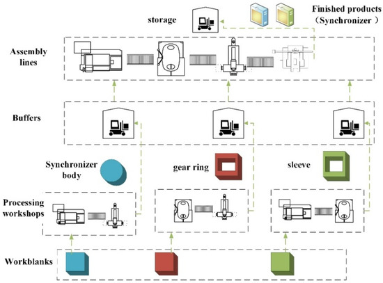
Figure 1.
Example of synchronizer production.
In the production process of the synchronizers, the production plan for the next month should be made according to the demand, making the best weekly production lot-sizing of each type of synchronizer and corresponding components to balance inventory and setup costs. The lot-sizing of every product per week is affected by external order requirements, product dependencies in BOM, and equipment production capacity. This problem can be described as an MIP model. Parameters and decision variables used in the model are defined as follows.
By using the notation in Table 1, Table 2 and Table 3, the lot-sizing problem we considered in synchronizer production can be formulated as follows:
s.t.

Table 1.
Indices and sets.

Table 2.
Parameters.

Table 3.
Decision variables.
3.2. Solving Model of MLCLSP with the Fuzzy-GA
When using the fuzzy-GA to deal with lot-sizing production problems, the general idea is to relax first. The capacity constraints are relaxed initially, the initial solution is obtained using the demand relationship, and the genetic operation is carried out. Then, the capacity constraint algorithm eliminates the solution that does not meet the constraints. The solution with the highest fitness is obtained on this basis and iterated several times until the optimization criteria are satisfied.
The MLCLSP solved in detail by the fuzzy-GA is given in Figure 2. First, the binary random variables are generated randomly, the initial lot-sizing is calculated, and stored as a hierarchical structure. Then, the capacity constraint algorithm is used to eliminate the individuals that do not meet the capacity constraint in the population, which is shown in Algorithm 1.
| Algorithm1 Capacity constraint algorithm |
| Input: xit, ; output: xit |
|
| {production lot size of period t is obtained without capacity constraints sort in ascending order . Then, find the minimum lot size . Calculate , Else calculate if . End this cycle and jump to Step 5 for the next cycle. End End |
|
| {the corresponding lot-sizing of is transferred to the production lot-sizing of . Set the corresponding binary variable to zero. Cyclic variable . Calculate }. |
|
| End |
|
|
If , jump to Step 4. Else, update . If , output updated lot-sizing, setup variable as result, and end the whole procedure; Else, the solution cannot satisfy the capacity constraint and end the whole procedure. End End |
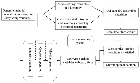
Figure 2.
Diagram of application of improved GA in lot-sizing production.
For individuals that satisfy capacity constraints, fitness value is calculated as follows: Using the variables, , xit, and Iit correspond to those meeting the capacity constraints to solve the target cost. The maximum value of all target costs in the population is selected and divided by the individual target cost as the individual fitness value. Algorithm 2 provides details of the algorithm.
| Algorithm 2 Algorithm of solving fitness value |
| Input: production lot-sizing x_it, inventory I_it, and setup variable Y_it; output: fitness value: f |
|
On the one hand, individuals with the largest fitness value were selected as the best solution and judged whether the iteration condition was satisfied. If it was satisfied, the algorithm ends and provides the result. If not, the algorithm continues to convert the decision variables of the hierarchy to single-layer binary strings hierarchical structure in preparation for genetic operations. On the other hand, the crossover and mutation probability was automatically adjusted according to fitness values combined with fuzzy theory. Finally, the roulette method is used for selection operation. The crossover and mutation operation adopts multipoint operation with the variable number of operation points determined by Formula (6).
where means to round to an integer, denotes the length of the chromosome to be interlaced or mutated, and is the proportional coefficient of operation point of mutation or crossover operation, which is a constant.
When the proposed algorithm is used to solve MLCLSP problems, the length of chromosomes is affected by the size of the production problem instance. Formula (6) ensures that the effects of crossover and mutation operations on population can be fully reflected when dealing with lot-sizing production problems of different scales. The fuzzy inference system obtains the mutation and crossover probability automatically during each iteration. The process of mutation operation and crossover operation is shown in Figure 3.
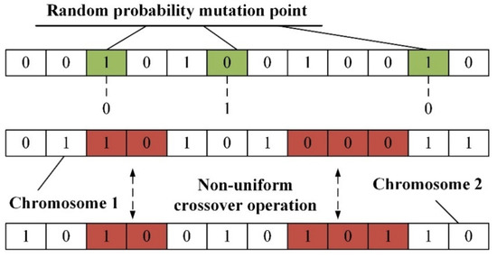
Figure 3.
Schematic diagram of crossover and mutation.
Compared with the traditional GA, the fuzzy-GA first uses the fuzzy reasoning system to calculate the crossover probability and mutation probability of an individual according to the fitness value in each iteration cycle before carrying out the genetic operation to realize the automatic adjustment of crossover and mutation probability in the genetic operation of each iteration.
3.3. Encoder Based on Hierarchical Structure
According to the planning period and product type, the initial population with size n is randomly generated, and the chromosome in the population is the binary string with length i × t corresponding to the setup variable . This binary string indicates whether the product i is produced during the planning period t. The specific relationship is shown in Figure 4. represents the product j at the BOM structure level i. Individuals in the population are arranged in sequence according to the plan period and then from top to bottom according to the BOM structure to form a binary string.
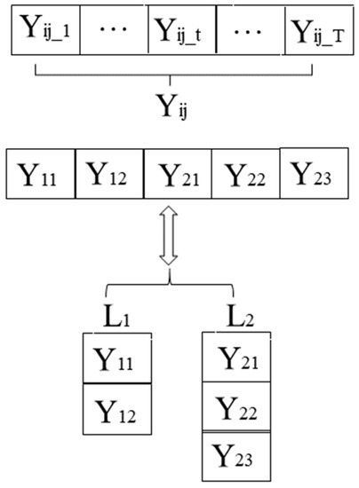
Figure 4.
Relational graph of encoding and multilevel structure.
The chromosome generated by 1 is stored as a hierarchical structure according to the product BOM. The conversion relationship of them is shown in Figure 4. The data of whether the product is ready for production in each planning period in the BOM are stored in each level. Taking , quantity dependence Rij, and external demand Dit as input variables, the lot-sizing algorithm constructed by demand relation (refer to Algorithm 3) is used to calculate the production decision variables xit.
| Algorithm 3 Algorithm of a lot-sizing solution according to the demand constraints |
| Input: setup variable, product demand, and material quantity relationship , , ; output: production lot-sizing |
|
| Use demand balance relation and solve production lot-sizing of product i at different planning periods. Else, use demand balance relation and solve production lot-sizing . End |
|
3.4. Adaptive Optimization Process of Parameters Based on Fuzzy Theory
The convergence and stability of the solution of traditional GAs are mainly affected by the crossover probability and mutation probability . and are fixed before the traditional GA runs, but they cannot be changed during the running process. During the algorithm’s operation, the same mutation and crossover rates are used regardless of the fitness value of individuals in the population. However, from the characteristics of the genetic algorithm, in each genetic operation, for individuals with high fitness, appropriately reducing the crossover rate and mutation rate is conducive to improving the convergence speed of the algorithm. For individuals with low fitness, appropriately increasing the value of the two is conducive to the global search of the solution, reducing the possibility of the solution converging to the local optimum. Aiming at the problem that the GA is easy to use to obtain an optimal local solution and unstable in solving lot-sizing production problems, this section proposes to apply a fuzzy reasoning system to control and . In each genetic operation, the fuzzy inference system is used to infer different crossover and mutation rates for individuals with different adaptive values to improve the global search ability and convergence speed of the algorithm.
Figure 5 shows the schematic diagram of the fuzzy reasoning system. In each iteration of the proposed algorithm, the maximum fitness value of the chromosome in the population is different, leading to the uncertainty of the input value range during the fuzzy reasoning process. Differences in the input value ranges of fuzzy inference systems correspond to different membership functions. To ensure that the input of the fuzzy reasoning process in each iteration has the same domain and is easy to be realized by programming, scale transformation mapping of input variables is needed. Therefore, when fuzzy reasoning is carried out in each iteration, combined with the characteristics of fitness value in each iteration, the following scale transformation formula is performed:
where represents the fitness value corresponding to the chromosome in the population of each iteration, represents the maximum of all fitness values in the population, and represents the output value after transformation. The same range of input variables is ensured in each reasoning process; they are all in the domain of [0, 1].
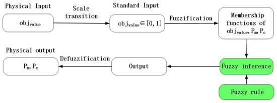
Figure 5.
Diagram of fuzzy reasoning system.
In the second step, the variables of input and output are fuzzified into fuzzy language variables by fuzzy set, which uses the mapping of membership function to describe the variables so that the same variable can belong to multiple sets but have different degrees of membership. Fuzzification can be divided into fuzzy division and membership function determination. Fuzzy partition determines the number of fuzzy sets on the domain. The higher the number of sets is, the more precise the association between fuzzy sets and precise quantities is. However, fine division quickly increases the amount of calculation. According to input and output characteristics, three fuzzy sets are divided in the input and output domain, namely, PS, PM, and PB, which indicate that the value is small, moderate, and large, respectively. The membership functions of all fuzzy sets are Gaussian functions commonly used in fuzzy reasoning, such as Formula (8), but different parameters are selected.
where is a variable in the domain, and parameters determine the rapid and slow change and the central position of the function curve, respectively.
In Formula (8), and are taken to obtain the small positive PS of the fuzzy language variable of input , which is represented by . Similarly, and can be substituted into Formula (8) to obtain the membership function corresponding to the positive middle PM of the input fuzzy language variable. The membership function of the fuzzy variable PM of the input can be obtained by making and in Formula (8).
In the proposed algorithm, the mutation probability value is small. Thus, in the fuzzy reasoning process, the range of mutation probability is [0, 0.003], [0, 0.03], or [0, 0.3]. The optimal range suitable for this problem will be determined by a trial method in Experiment 2 of the paper. Then, taking different and values for Formula (8) in the experiment, we can obtain the membership function , , and corresponding to fuzzy language variables PB, Pm, and PS of output , respectively.
The domain of output crossover probability in fuzzy inference system is [0, 1]. In Formula (8), . In Experiment 2, the values of membership functions , and corresponding to fuzzy language PB, and PM and PS for are discussed.
Then, according to the fuzzy rules, the fuzzy input can obtain the fuzzy output through fuzzy reasoning. Finally, after defuzzification, the output can give the actual crossover probability and mutation probability output. The primary purpose of defuzzification is to transform the fuzzy output from fuzzy reasoning into the available actual production. In the algorithm, the centroid method is used as the defuzzification method, as shown in Formula (9):
where is the domain of output mutation or crossover probability. is membership function of fuzzy sets in the domain. represents the output after defuzzification.
In the implementation process, fuzzy inference and the establishment of fuzzy rules are the core steps, which are the green boxes shown in Figure 5.
Fuzzy rules are expert experiences or known rules expressed by fuzzy language variables. Through observation, in the iteration process of the algorithm, when the fitness value , is small, slightly increasing the mutation rate or increasing crossover probability can improve the global search ability of the algorithm. When the fitness value is large, appropriately decreasing mutation rate or crossover probability can improve the convergence speed of the algorithm and improve the stability of the solution. The rules expressed by if−then are as follows:
If is PS, then and are PB.
If is PM, then and are PM.
If is PB, then and are PS.
A fuzzy control table can be obtained according to the above empirical rules, as shown in Table 4.

Table 4.
Rules of fuzzy inference.
Fuzzy reasoning is the process of obtaining the fuzzy output of the system by using fuzzy logic operations, such as implication and synthesis according to the fuzzy rules. The fuzzy relation model Rm and Rc of output Pm and Pc that is based on the max−min composition rule can be expressed as follows:
where intersection represents the smaller value of two operands and union indicates finding the maximum value of the two operands.
Formula 10 is established with fuzzy rules in Table 4. The operation within rules takes intersection, and the operation between rules takes union. Fuzzy decision-making is performed by the fuzzy relation model, which determines the output of the fuzzy system by combining the input of the fuzzy system with the fuzzy reasoning model. As shown in Formula (11),
where and denote the membership function of output and denotes the membership function of the input.
4. Experimental Setup
4.1. Experimental Data and Design Hypothesis
This study designs three experiments to verify the algorithm’s effectiveness, find the optimal parameters of the fuzzy reasoning algorithm, and illustrate the comprehensive performance of the algorithm. The experimental results are obtained in the environment of i5-7200U 2.71 GHz CPU and 4.00 GB memory, running MATLAB programming software version R2014b and the commercial software lingo 11.0.0.20.
4.1.1. Experiment 1 Validation of Fuzzy-GA in Solving MLCLSP
A two-level BOM material structure is constructed based on an actual production line of a synchronizer. The first level is composed of products 1 and 2. The second level is composed of products 3, 4, and 5. The proposed algorithm and the commercial software lingo were compared to verify the solution results. The production costs obtained from both methods are calculated to verify the algorithm’s effectiveness. Table 5 shows the production demand of product in planning period .

Table 5.
Product demand .
Table 6 shows the production capacity of the equipment in each planning period. Table 7 lists the quantity relationship between the secondary products and the primary products in the BOM.

Table 6.
Capacity of production devices .

Table 7.
Product assembly ratio in BOM.
The production setup time and the unit production time of product on the equipment at period are shown in Table 8. Other parameters of the example, unit production cost, inventory cost, production setup cost, and initial inventory are given in Table 9.

Table 8.
Time cost \ of setup\production per unit.

Table 9.
Other model parameters.
4.1.2. Experiment 2 Adaptive Parameters of the Fuzzy-GA
In this experiment, the dataset from Experiment 1 is still used. The central parameters of the output membership function greatly influence the algorithm performance in the fuzzy reasoning system. Thus, the parameters suitable for crossover probability and mutation probability are determined in the process of solving the MLCLSP with the proposed algorithm. Multiple sets of values are used to solve the problem. By comparing the results, the better operation parameters of the algorithm are given.
Table 10 shows the specific values of the central control parameters of the membership functions in the language variable set corresponding to the mutation probability in the fuzzy reasoning system in three cases, , which represent parameters of different orders of magnitude.

Table 10.
Parameters of mutation with different magnitudes.
Table 11 shows the specific values of the central control parameters of each membership function in the language variable set corresponding to the crossover probability in the fuzzy reasoning system under three cases . A PM equal to 0.7 means that the chromosome crossover probability of the intermediate fitness value tends to be large in each iteration population. A PM equal to 0.3 means that the chromosome crossover probability of the intermediate fitness value tends to be small in each iteration population. A PM equal to 0.5 is between the two.

Table 11.
Parameters of crossover with different magnitude.
4.1.3. Experiment 3 Performance of Fuzzy-GA in Solving MLCLSP
On the basis of the production examples of different scales, the MLCLSP was solved by GA and the proposed algorithm, and the superiority of the proposed algorithm was verified. This experiment mainly verifies whether the algorithm’s speed, quality, and stability are improved for the proposed algorithm in solving the MLCLSP. The response speed of the improved algorithm is verified by comparing the solution time. The comparison of the best solution is used to verify the quality of the solution. The difference between the average and the best solution is used to verify the stability of the solution.
Computational experiments were conducted on three groups of test instances (i.e., N(5,10,20)-T5-M9, N20-T(5,7,10)-M9, and N20-T10-M(9,15,20), representing different problem scales, where the numbers represent products, periods, and machines, respectively). These groups are similar to the data structure of Experiment 1. N(5,10,20) means N5, N10, and N20. Thus, each combination has three instances, producing seven instances in total. According to the synchronizer generation process, all instances have a two-level BOM structure. Although the real-life data are unavailable because of confidentiality, the setting of those instances was simulated from the practice in a production line of a synchronizer assembly manufacturing company in China.
4.2. Performance Evaluation Metrics
Different performance characteristics require different methods to measure. This study mainly examined the effectiveness, optimal parameter selection, and stability of the algorithm. Thus, the corresponding measurement methods for these performance characteristics are given below.
The proposed algorithm is a random algorithm, which has a certain difference in the results of each solution for the same instance. The optimal total cost of the MLCLSP solved by the proposed algorithm is the expected value of n calculations as follows:
Assuming that the optimal cost of the commercial software lingo solution is denoted as , then the effectiveness of the proposed algorithm can be measured by Formula (13).
Adjusting the mutation probability can improve the defect that easily falls into the optimal local solution for the GA. Thus, the selection of the central parameters of the output membership function of mutation rate takes the minimum value of the optimal cost under different parameters as the measurement index. Assuming that is the optimal cost of the proposed algorithm in the case of , the measurement index can be written as follows:
Adjusting the crossover probability can improve the stability of the solution, which means the amplitude of the target value will weaken as the number of iterations increases. Thus, the central parameters of the output membership function of crossover rate with the highest density of curves is selected as the best parameter, according to the different densities of curves in the figure of optimization target changing with the number of iterations under the case of different .
In Experiment 3, the optimal value of different scales takes the minimum objective value of multiple solutions as Formula (15). The average optimal value is the expected value of various solutions, which can be expressed by Formula (12).
The stability of the proposed algorithm can be expressed by the difference between the average value and the best value as Formula (16).
Assuming that elapsed time of the proposed algorithm denotes , the proposed algorithm’s computational speed is measured by the average speed of multiple algorithm solutions, as shown in Formula (17).
5. Results and Discussion
5.1. Results and Discussion for Experiment 1
The number of iterations is 100, and the population size is 30. The proportional coefficient of mutation operation , the proportional coefficient of crossover operation , and and in the fuzzy reasoning system are selected. Using the proposed algorithm, the optimal value of comprehensive cost is 18,320 by running the example, and the corresponding lot-sizing production results are shown in Table 12.

Table 12.
Production lot-size under optimal objective value.
Verifying that the production lot size can meet external demand in Table 5, and capacity requirements in Table 6 are easy, indicating the algorithm’s feasibility. The commercial soft lingo is used for solving, and the optimal value is 18,203. The difference is 150, and the relative error is 0.639% between the two, which shows the proposed algorithm’s effectiveness.
As shown in Figure 6, the legend number corresponds to the product number. The abscissa is the production planning period. The ordinate is the product production quantity, which shows the production quantity change rule of various products in the same planning period. Figure 7 reflects the proportion distribution of energy consumption of different products in the total energy consumption in each period, where the different colors are consistent with Figure 6. Combining Figure 6 and Figure 7, the distributions of energy consumption are consistent with the size of product lot-sizing but show some differences, such as products 4 and 5 in the fourth period, mainly caused by the difference in energy consumption costs between them.
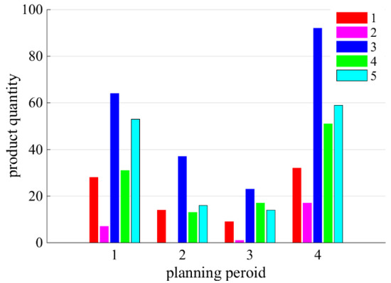
Figure 6.
Column diagram of production quantity of different planning periods.
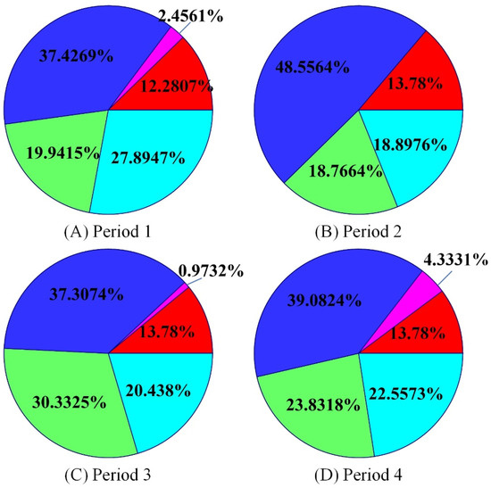
Figure 7.
Energy costs of all products for: (A) planning period 1; (B) planning period 2; (C) planning period 3; (D) planning period 4.
The legend number in Figure 8 corresponds to the production planning period, the abscissa is the product type number, and the ordinate is the product production quantity. Figure 8 describes the production quantity of the same product in a different production period. Through the classified display of the two results, the lot-sizing distribution of different products in each planning period can be displayed clearly. Figure 9 shows the proportion of energy consumption of each period in the total energy consumption for various products, in which the different colors are consistent with Figure 8. Comparing Figure 8 and Figure 9, different products have a large proportion of energy consumption in period 4. Thus, optimizing energy consumption can focus on the planning of period 4.
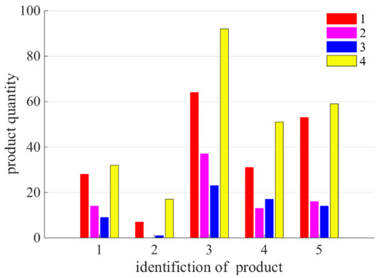
Figure 8.
Quantity column diagram of different productions.
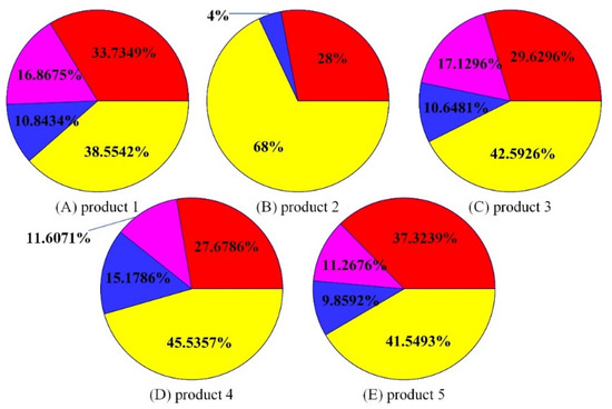
Figure 9.
Energy costs of synchronizers for: (A) product 1; (B) product 2; (C) product 3; (D) product 4; (E) product 5 in the planning horizon.
5.2. Results and Discussion for Experiment 2
The results in Figure 10 are randomly run five times and are drawn by taking the minimum target value in each case. Three smooth curves are the fitting results of three actual curves in the figure, obtained using a six-order polynomial function. The fitting curve shows that the variation trend of the solution tends to be flat and the worst effect of the optimal solution is when the magnitude of the mutation parameter is too small. When the magnitude of the mutation parameter is the largest, as shown in the curve , the change of the target value has a sharp convergence with the number of iterations, and the overall target value tends to decrease. However, the final convergence result is poorer than curve . When the mutation parameter takes the middle value, according to the curve , the intensity of the overall trend of the target value is slightly worse than that of curve , but the effect of the optimal solution is the best of the three. Thus, when the proposed fuzzy-GA is used to solve a lot-sizing problem, groups of parameters can be selected.
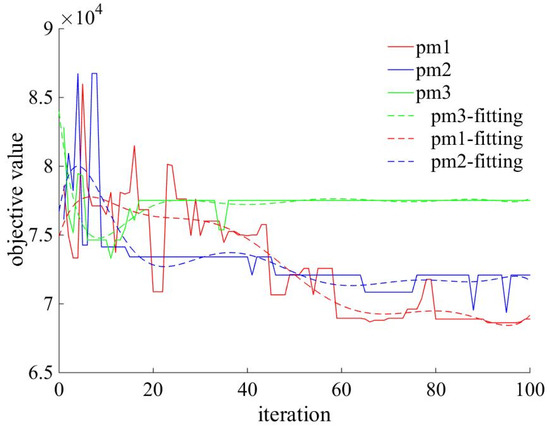
Figure 10.
Comparison of results with different parameters of mutation.
Figure 11, Figure 12 and Figure 13 show the parameters in the case of When the fuzzy-GA is run many times, the target value changes with the number of iterations. Compared with , the trend of the curves between the target value and the number of iterations is better. Although the optimal results are close to each other with different parameters, the curves are more concentrated in the case of , , and and are relatively scattered. Therefore, the fuzzy-GA algorithm has better stability for lot-sizing problem solving under the parameter of .
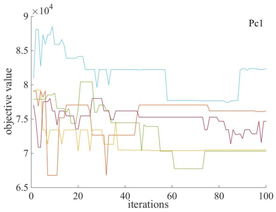
Figure 11.
Results with parameters Pc1 of crossover.
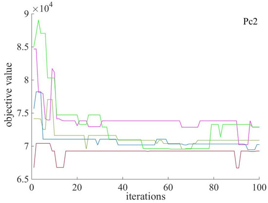
Figure 12.
Results with parameters Pc2 of crossover.
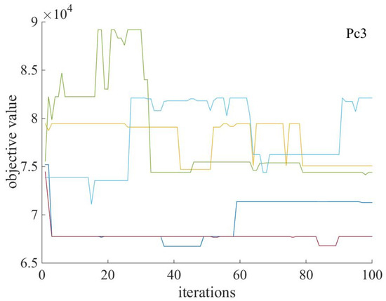
Figure 13.
Results with parameters of Pc3 crossover.
5.3. Results and Discussion for Experiment 3
In this experiment, the parameter of the mutation probability membership function adopts , and the parameter of the crossover probability membership function adopts . Table 13 shows the results of solving the MLCLSP by the general GA and the fuzzy-GA, which includes different production scales indicated by product type, planning period, and the number of devices.

Table 13.
Comparison of results between GA and fuzzy-GA.
The iterations in Table 13 represent the average number of iterations for 10 runs of the algorithm. Iterations are the number of iterations based on the criterion that the optimization objective has not been optimized for 50 consecutive times during the algorithm’s operation. The average optimal value and running time in Table 6 are the average value of the algorithm running 10 times. The optimal value is the minimum of 10 running results. The smaller the target value, the better the performance of the corresponding lot-sizing solution. The table shows that, when the planning period and the number of devices are the same, with the increase in product types, fuzzy-GA’s optimal value is smaller than that of the traditional GA. Therefore, the improved genetic algorithm has better optimization ability for different product types. The average optimal value of the fuzzy-GA is smaller when the production scale is the same, which indicates that the improved genetic algorithm still shows superior stability. At the same time, the number of iterations fluctuates less, and the running time is less, which shows that the algorithm has better stability for the increase in product types in solving lot-sizing problems. Table 13 also shows that, when the product type and the number of pieces of equipment are fixed, compared with the traditional GA, the optimal value and average optimal value of the fuzzy-GA are smaller, which indicates that the result performance of the improved genetic algorithm is better when the scale of the planning period is increased. The iterations of the two algorithms have slight fluctuation, and the running time is similar, which indicates that the running time of the two algorithms is relatively stable when the scale of the planning period increases, but the running time of the improved algorithm is slightly shorter. When product types and planned periods are fixed, Table 13 shows that, with the increase in the number of devices, the improved genetic algorithm solution has a better effect, the iteration times are more stable, and the algorithm runs faster.
In general, with the increase in the number of products, planning periods, and devices, compared with the traditional GA, the fuzzy-GA has a better effect on the optimal and average values of the target, more stable iterations, and less running time.
Table 14 shows the optimal value and running time of calculation examples of different scales under the proposed iteration stop condition, iteration 100 times, iteration 300 times, and iteration 500 times, respectively. In order to reduce the influence caused by the randomness of the algorithm, the optimal value is the optimal value of 10 calculations, and the running time is the average of 10 calculations. As can be seen from Table 14, when the number of iterations is constant, the iteration time increases with the increase of production scale. At the same scale, the optimal value becomes better and better with the increase of iterations, but calculation time is also increasing. Under different scales, the optimal value of the proposed stop condition of iteration is similar to the result performance of 300 iterations, but requires less calculation time.

Table 14.
Results of different iterations with fuzzy-GA.
Table 15 presents the performance comparison with other methods; the mean of iterations indicates the average number of iterations the algorithm runs to obtain the best value in all calculation examples. This indicator reflects the search capability of the algorithm. References [4,21] do not give the number of iterations of the algorithm. The mean of deviation is the expected ratio between the average and best values of the calculation examples in the dataset and the average values. This indicator can reflect the possibility of obtaining the optimal global solution of the algorithm. The smaller the value is, the greater the likelihood of obtaining the optimal solution during each algorithm operation. The range of variation indicates the difference between the maximum and the minimum values of the deviation, reflecting the fluctuation range of understanding. The smaller the value of the indicator, the more stable the solution. These two indicators together reflect the algorithm’s global search capability and stability. Table 15 reveals that each proposed algorithm indicator is superior to the algorithm in references [21,39] and the PSO algorithm in reference [4]. Compared with the GLNPSO algorithm in reference [4], the global optimization ability of the proposed literature is slightly worse, but the stability of the solution is better.

Table 15.
Performance comparison with other methods.
6. Conclusions and Prospects
This study realizes solving the MLCLSP by the fuzzy-GA, which analyzes the results of different values of parameters of mutation membership function and crossover membership function in the fuzzy-GA and gives the specific parameters suitable for the MLCLSP. In the different production scales, the GA and the fuzzy-GA are run, and the optimal solution, the average value of the optimal solution, the iterations, and the running time are recorded. Compared with the traditional GA, the proposed algorithm can improve the solution speed, stability, and accuracy of the solution. The distribution of energy consumption is given for the case of the production of the synchronizer, which can provide a reference for relevant enterprises to reduce energy consumption.
Although the setup time is considered in the MLCLSP, the setup carryover during the planning period is not considered in order to reduce the difficulty of problem-solving, which actually exists in the synchronizer production. Moreover, the scheduling optimization in each planning period is also not considered when dealing with the MLCLSP in this study. Therefore, the proposed algorithm in this paper may not be effective for such cases. Future work will focus on improving algorithms which can be used to solve the MLCLSP with setup carryover or scheduling optimization.
Author Contributions
Conceptualization, S.W. and B.Z.; funding acquisition, J.H.; methodology, S.W.; project administration, J.H.; supervision, J.H.; writing—original draft, S.W.; writing—review and editing, B.Z. and Y.L. All authors have read and agreed to the published version of the manuscript.
Funding
This research was funded by the intelligent manufacturing support project for major science and technology programs of Shaanxi Province grant number Grant No. 2018zdzx01-01-01.
Institutional Review Board Statement
Not applicable.
Informed Consent Statement
Not applicable.
Data Availability Statement
The data involved in this study are available through the corresponding author.
Acknowledgments
The authors are grateful to the financial support of the intelligent manufacturing support of the intelligent manufacturing support project for major science and technology programs of Shaanxi Province (Grant No. 2018zdzx01-01-01).
Conflicts of Interest
The authors declare no conflict of interest.
References
- Awad, M.I.; Hassan, N.M. Joint decisions of machining process parameters setting and lot-size determination with environmental and quality cost consideration. J. Manuf. Syst. 2018, 46, 79–92. [Google Scholar] [CrossRef]
- Jia, S.; Yuan, Q.; Cai, W.; Li, M.; Li, Z. Energy modeling method of machine-operator system for sustainable machining. Energy Convers. Manag. 2018, 172, 265–276. [Google Scholar] [CrossRef]
- Klement, N.; Abdeljaouad, M.A.; Porto, L.; Silva, C. Lot-Sizing and Scheduling for the Plastic Injection Molding Industry—A Hybrid Optimization Approach. Appl. Sci. 2021, 11, 1202. [Google Scholar] [CrossRef]
- Boonmee, A.; Sethanan, K. A GLNPSO for multi-level capacitated lot-sizing and scheduling problem in the poultry industry. Eur. J. Oper. Res. 2016, 250, 652–665. [Google Scholar] [CrossRef]
- Berretta, R.; Rodrigues, L.F. A memetic algorithm for a multistage capacitated lot-sizing problem. Int. J. Prod. Econ. 2004, 87, 67–81. [Google Scholar] [CrossRef]
- Buschkühl, L.; Sahling, F.; Helber, S.; Tempelmeier, H. Dynamic capacitated lot-sizing problems: A classification and review of solution approaches. Or Spectr. 2010, 32, 231–261. [Google Scholar] [CrossRef]
- Duda, J.; Stawowy, A. Optimization Methods for Lot-Sizing Problem in an Automated Foundry. Arch. Metall. Mater. 2013, 58, 863–866. [Google Scholar] [CrossRef][Green Version]
- Jia, S.; Yuan, Q.; Lv, J.; Liu, Y.; Ren, D.; Zhang, Z. Therblig-embedded value stream mapping method for lean energy machining. Energy 2017, 138, 1081–1098. [Google Scholar] [CrossRef]
- Jinxing, X.; Jiefang, D. Heuristic genetic algorithms for general capacitated lot-sizing problems. Comput. Math. Appl. 2002, 44, 263–276. [Google Scholar]
- Yijun, L.; David, L. Self-adaptive randomized constructive heuristics for the multi-item capacitated lot-sizing problem. arXiv 2021, arXiv:2103.04199. [Google Scholar]
- Furlan, M.M.; Santos, M.O. BFO: A hybrid bees algorithm for the multi-level capacitated lot-sizing problem. J. Intell. Manuf. 2017, 28, 929–944. [Google Scholar] [CrossRef]
- Kirschstein, T.; Meisel, F. A dynamic multi-commodity lot-sizing problem with supplier selection storage selection and discounts for the process industry. Eur. J. Oper. Res. 2019, 279, 393–406. [Google Scholar] [CrossRef]
- Cunha, J.O.; Kramer, H.H.; Melo, R.A. On the computational complexity of uncapacitated multi-plant lot-sizing problems. Optim. Lett. 2021, 15, 803–812. [Google Scholar] [CrossRef]
- Han, Y.; Kaku, I.; Tang, J.; Dellaert, N.; Cai, J.; Li, Y. A Comparison of Particle Swarm Optimizations for Uncapacitated Multilevel Lot-sizing Problems(Theory and Methodology). J. Jpn. Ind. Manag. Assoc. 2010, 61, 203–213. [Google Scholar]
- Seeanner, F. Multi-Stage Simultaneous Lot-Sizing and Scheduling—Planning of Flow Lines with Shifting Bottlenecks; Springer Science & Business Media: Berlin/Heidelberg, Germany, 2013. [Google Scholar] [CrossRef]
- Jia, S.; Yuan, Q.; Cai, W.; Lv, J.; Hu, L. Establishing prediction models for feeding power and material drilling power to support sustainable machining. Int. J. Adv. Manuf. Technol. 2019, 100, 2243–2253. [Google Scholar] [CrossRef]
- Jia, S.; Cai, W.; Liu, C.; Zhang, Z.; Bai, S.; Wang, Q.; Li, S.; Hu, L. Energy modeling and visualization analysis method of drilling processes in the manufacturing industry. Energy 2021, 228, 120567. [Google Scholar] [CrossRef]
- Zohali, H.; Naderi, B.; Mohammadi, M. The economic lot scheduling problem in limited-buffer flexible flow shops: Mathematical models and a discrete fruit fly algorithm. Appl. Soft Comput. 2019, 80, 904–919. [Google Scholar] [CrossRef]
- Farooq, B.; Bao, J.; Raza, H.; Sun, Y.; Ma, Q. Flow-shop path planning for multi-automated guided vehicles in intelligent textile spinning cyber-physical production systems dynamic environment. J. Manuf. Syst. 2021, 59, 98–116. [Google Scholar] [CrossRef]
- Che, Z.H.; Chiang, T.A.; Lin, T.T. A multi-objective genetic algorithm for assembly planning and supplier selection with capacity constraints. Appl. Soft Comput. 2021, 101, 107030. [Google Scholar] [CrossRef]
- Hadi, A.S.; Mehdi, R.B. Solving a flexible job shop lot sizing problem with shared operations using a self-adaptive COA. Int. J. Prod. Res. 2021, 59, 483–515. [Google Scholar]
- Andrés, A.; Mingyuan, C. Multi-level lot-sizing with raw-material perishability, deterioration, and lot-sizing ordering: An application of production planning in advanced composite manufacturing. Comput. Ind. Eng. 2020, 145, 106484. [Google Scholar]
- Sikora, R. A genetic algorithm for integrating lot-sizing and sequencing in scheduling a capacitated flow line. Comput. Ind. Eng. 1996, 30, 969–981. [Google Scholar] [CrossRef]
- Soltanali, H.; Rohani, A.; Tabasizadeh, M.; Abbaspour-Fard, M.H.; Parida, A. An improved fuzzy inference system-based risk analysis approach with application to automotive production line. Neural Comput. Appl. 2020, 32, 10573–10591. [Google Scholar] [CrossRef]
- Tempelmeier, H.; Helber, S. A heuristic for dynamic multi-item multi-level capacitated lot-sizing for general product structures. Eur. J. Oper. Res. 1984, 75, 296–311. [Google Scholar] [CrossRef]
- Boctor, F.F.; Poulin, P. Heuristics for N-product, M-stage, economic lot sizing and scheduling problem with dynamic demand. Int. J. Prod. Res. 2005, 43, 2809–2828. [Google Scholar] [CrossRef]
- Miller, A.J.; Nemhauser, G.L.; Savelsbergh, M. Solving Multi-Item Capacitated Lot-Sizing Problems with Setup Times by Branch-and-Cut; CORE Discussion Papers; Université Catholique de Louvain: Ottignies-Louvain-la-Neuve, Belgium, 2000. [Google Scholar]
- Zhang, C.; Zhang, D.; Wu, T. Data-driven Branching and Selection for Lot-sizing and Scheduling Problems with Sequence-dependent Setups and Setup Carryover. Comput. Oper. Res. 2021, 132, 105289. [Google Scholar] [CrossRef]
- Ramezanian, R.; Saidi-Mehrabad, M.; Fattahi, P. MIP formulation and heuristics for multi-stage capacitated lot-sizing and scheduling problem with availability constraints. J. Manuf. Syst. 2013, 32, 392–401. [Google Scholar] [CrossRef]
- Verma, M.; Sharma, R. Lagrangian relaxation and bounded variable linear programs to solve a two-level capacitated lot sizing problem. In Proceedings of the 2011 3rd International Conference on Electronics Computer Technology, Kanyakumari, India, 8–10 April 2011; Volume 6, pp. 188–192. [Google Scholar]
- Tempelmeier, H.; Buschkühl, L. A heuristic for the dynamic multi-level capacitated lot-sizing problem with linked lot-sizes for general product structures. Or Spectr. 2009, 31, 385–404. [Google Scholar] [CrossRef]
- Wu, T.; Shi, L.; Geunes, J.; Akartunalı, K. An optimization framework for solving capacitated multi-level lot-sizing problems with backlogging. Eur. J. Oper. Res. 2011, 214, 428–441. [Google Scholar] [CrossRef]
- Zhao, Q.; Xie, C.; Xiao, Y. A variable neighborhood decomposition search algorithm for multi-level capacitated lot-sizing problems. Electron. Notes Discret. Math. 2012, 39, 129–135. [Google Scholar] [CrossRef]
- Chen, H. Fix-and-optimize and variable neighborhood search approaches for multi-level capacitated lot sizing problems. Omega 2015, 56, 25–36. [Google Scholar] [CrossRef]
- Mohammadi, M.; Fatemi Ghomi SM, T.; Karimi, B.; Torabi, S.A. Rolling-horizon and fix-and-relax heuristics for the multi-product multi-level capacitated lot-sizing problem with sequence-dependent setups. J. Intell. Manuf. 2010, 21, 501–510. [Google Scholar] [CrossRef]
- Pitakaso, R.; Almeder, C.; Doerner, K.F.; Hartl, R.F. Combining exact and population-based methods for the constrained multi-level lot-sizing problem. Int. J. Prod. Res. 2006, 44, 4755–4771. [Google Scholar] [CrossRef]
- Toledo, C.F.M.; De Oliveira, R.R.R.; França, P.M. A Hybrid Multi-Population Genetic Algorithm Applied to Solve the Multi-Level Capacitated Lot Sizing Problem with Backlogging; Elsevier Science Ltd.: Amsterdam, The Netherlands, 2013; Volume 40, pp. 910–919. [Google Scholar]
- Mohammadi, M.; Ghomi, S.M.T.F. Genetic algorithm-based heuristic for capacitated lot-sizing problem in flow shops with sequence-dependent setups. Expert Syst. Appl. 2011, 38, 7201–7207. [Google Scholar] [CrossRef]
- Duda, J. A hybrid genetic algorithm and variable neighborhood search for multi-family capacitated lot-sizing problem. Electron. Notes Discret. Math. 2017, 58, 103–110. [Google Scholar] [CrossRef]
- Quadt, D.; Kuhn, H. Capacitated lot-sizing with extensions: A review. 4OR 2008, 6, 61–83. [Google Scholar] [CrossRef]
Publisher’s Note: MDPI stays neutral with regard to jurisdictional claims in published maps and institutional affiliations. |
© 2022 by the authors. Licensee MDPI, Basel, Switzerland. This article is an open access article distributed under the terms and conditions of the Creative Commons Attribution (CC BY) license (https://creativecommons.org/licenses/by/4.0/).