Review on Millimeter-Wave Radar and Camera Fusion Technology

Abstract

Cameras allow for highly accurate identification of targets. However, it is difficult to obtain spatial position and velocity information about a target by relying solely on images. The millimeter-wave radar (MMW radar) sensor itself easily acquires spatial position and velocity information of the target but cannot identify the shape of the target. MMW radar and camera, as two sensors with complementary strengths, have been heavily researched in intelligent transportation. This article examines and reviews domestic and international research techniques for the definition, process, and data correlation of MMW radar and camera fusion. This article describes the structure and hierarchy of MMW radar and camera fusion, it also presents its fusion process, including spatio-temporal alignment, sensor calibration, and data information correlation methods. The data fusion algorithms from MMW radar and camera are described separately from traditional fusion algorithms and deep learning based algorithms, and their advantages and disadvantages are briefly evaluated.

1. Introduction

MMW radar corresponds to electromagnetic waves with a frequency range from 30~300 GHz and a vacuum wave length from 0.1~1.0 cm. Its unique frequency range gives it better penetration in radar detection, allowing it to easily penetrate snow, smoke, dust, etc., with the ability to work all-weather in extreme environments. Based on its all-weather and even space exploration applications and other reconnaissance advantages, scientists have conducted a great deal of research into its application in the field of precision navigation, particularly in military applications such as radar guidance heads for missiles [1] and gunfire control and tracking of low-altitude targets [2]. Based on its good performance, MMW radar is used in vehicle radar [3], intelligent robots [4], biological sign recognition [5], gesture recognition [6], and so on. However, MMW radar also has some defects, firstly, MMW radar is susceptible to interference from electromagnetic waves, detection is sparse, and the density of detection is not sufficient to represent the physical characteristics of the target, like lines and angles, it is also not to mention detecting lanes and pedestrians. Secondly, the low accuracy of MMW radar leads to ambiguity in the manual interpretation of measurement data, which makes the data tagging process become more difficult and expensive. Finally, without large amounts of high-quality labelled training data, it is difficult to ensure that supervised machine learning models can predict, classify or analyse phenomena of interest with the required accuracy.

The camera has a good ability to discriminate the features of the target and is good at identifying all stationary and moving objects such as pedestrians and vehicles and is good at providing spatial information about the object. In the past few decades, computer vision has combined computer, geometric, optical and psychological, etc., and has had a wide range of applications in professions such as industry [7], agriculture [8], medicine [9], military [10], aerospace [11], public security [12] and transportation [13], and is still gradually expanding. However, it has a short field of vision and is affected by extreme weather, dim light, and other conditions. It can be “blind” in rain, fog, and darkness, and it does not work properly in strong or low light.

In summary, MMW radar offers relatively high distance resolution, but it has a lower resolution in terms of orientation (azimuth/elevation). Compared to MMW radar, the camera offers high spatial resolution but is less accurate in estimating object distances. It can be seen that MMW radar and camera sensors are complementary, and the fusion of MMW radar data and camera data can make good use of the information provided by the different sensors to complement each other, reducing the reliance on individual sensors and making the fused information richer and more comprehensive. The fusion of MMW radar and vision sensors facilitates image recognition by using MMW radar for accurate range and angle measurement of targets and vision sensors for classification of targets detected by MMW radar, improving the detection capability of the detection system under different environmental and climatic conditions.

2. Materials and Methods

2.1. MMW Radar and Camera Information Fusion Technology

2.1.1. Definition of MMW Radar and Camera Information Fusion

MMW radar and camera information fusion is the fusion of MMW radar point cloud information and image video information, from the fused information to obtain the point cloud position of the object, the velocity and acceleration of the object, as well as the shape and relative distance of the object. The fusion of MMW radar and camera mainly consists of spatio-temporal fusion and velocity fusion. The accuracy of the fusion algorithm determines the fusion result.

2.1.2. MMW Radar and Camera Information Fusion Architecture

Information fusion [14] as the integrated processing of multiple MMW radar and camera information is intrinsically complex, currently, the main fusion structures for MMW radar and cameras are divided into three types: centralized fusion, distributed fusion, and hybrid fusion. Their main fusion structures, advantages and disadvantages are shown in the following

Table 1. Advantages and disadvantages of each fusion structure.

Fusion Structure	Definition	Advantages	Disadvantages
Centralised convergence	The centralised fusion architecture means that the raw data obtained by each MMW radar and camera is sent directly to the central processor for fusion processing, which allows for real-time fusion.	The structure has a low information loss rate and largely preserves the original data, it has a simple structure, high data processing accuracy, relatively flexible algorithms and fast fusion.	Each MMW radar and camera is independent of each other and the data flows directly to the fusion centre without the necessary connection; the method requires a large communication bandwidth for transmission and requires the fusion centre to have a high information processing computing power. The fusion centre is overloaded with computing and communication, the system is poorly fault tolerant and less reliable.
Distributed Convergence	In a distributed fusion architecture, each MMW radar and camera locally processes the raw data, makes an initial prediction and then sends the results separately to the fusion centre for fusion and finally obtains the target results.	Each MMW radar and camera in this approach has the ability to estimate global information, reducing the transmission and computing pressure on the fusion centre. Failure of any one MMW radar or camera will not cause the system to crash, resulting in high system reliability and fault tolerance. And with its low communication bandwidth requirements, fast computing speed, reliability and continuity, this fusion architecture has also become more popular with researchers in recent years.	Each MMW radar and camera requires an application processor, which is larger and more power-efficient; and the central processor can only access the processed object data from the individual sensors, not the raw data.
Hybrid integration	A hybrid architecture, a mixture of centralised and distributed applications, where some sensors use a centralised fusion architecture and the remaining sensors use a distributed one. Measurements from multiple sensors for each target are combined into a hybrid measurement, and the hybrid measurement is then used to update the full data.	The hybrid converged architecture retains the advantages of both centralised and distributed architectures, allowing for flexibility in fulfilling task requirements in different situations and a high degree of usability.	Hybrid sensor fusion has a more complex structure, increasing the communication and computational load, but it requires high structural design requirements for communication bandwidth and computational power, and the system is instable.

.

2.1.3. Layers of MMW Radar and Camera Data Fusion

The differences between radar fusion systems and visual fusion systems are mainly in the level of fusion and the synchronous or asynchronous processing schemes. Alessandretti et al. [15,16] have classified the level of fusion into three levels, including low, medium, and high levels, and have achieved good results with all.

• The low level is data-level fusion, where low-level fusion combines several sources of raw data to produce new raw data.
• Medium level fusion, which is target level fusion, which combines various features, such as edges, corners, lines, texture parameters, etc., into a feature map that is then further processed.
• Advanced fusion, also known as decision-level fusion, where each input source produces a decision and finally all decisions are combined.

Data Level Convergence

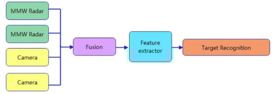
Data layer fusion of MMW radar data and camera data is the fusion of radar point clouds and image pixels, sometimes called pixel-level fusion, where MMW radar and camera observed data are fused directly without pre-processing. The aim of this method is to fuse the original MMW radar data and camera data and then produce new raw data, which contains more useful information within the new fused data. The specific operation method is to project the coordinate of the radar data onto the image pixels and matching them with the joint calibration of the image pixels. Feature extraction and classification is then performed on the fused data. The process framework is shown in the Figure 1.

The advantages of MMW radar and cameras fuse at the data level are that it ensures data integrity, provides subtle information that is not available at other fusion levels, and has a high correlation between data. However, no pre-processing of the raw data leads to high data redundancy, poor real-time performance, poor interference immunity and high bandwidth requirements during communication; on the other hand, fusion is carried out at the lowest layer of information, which has high requirements for error correction ability. The common fusion methods of pixel layer are weighted average method and Kalman filter method. This technique is widely used in road traffic and has achieved corresponding success.

As the fusion of the MMW radar data and the camera data is mostly asynchronous at the data level, temporal data calibration using a set of filters for interpolating data is required for data fusion, followed by correlating data from multiple sensors, associating observations from MMW radar and vision sensors with different targets through a variety of algorithms that are feasible for efficient classification. Finally dynamic target can be tracked and estimated, at present, Kalman filter is widely used to estimate the target state.

Grover et al. [17] fused the low-level features which was detected in radar data and visual data in 2001 using a single radar map and a single night vision image, the fusion was in polar coordinates and based on angular position. Steux [18] developed a fusion system that automatically combines the results of four different image processing algorithms with 12 different features to fuse radar information and generates multiple possible target location suggestions. In the same year, Fang and Masaki [19] proposed a target detection method that fuses target depth information with binocular stereo images. Typically, radar can provide the required target depth and information from the radar sensor (coarse depth) is used to guide the processing (segmentation) of the video sensor. The reliability of the algorithm is improved by decomposing the multi-target segmentation task into multiple single-target segmentation tasks on a depth-based target feature layer. Shigeki et al. [20] proposed a method to segment the radar-acquired data into clusters and visualise the radar-acquired target information on image sequences using the single-strain nature of the transformation between the radar plane and the image plane in 2004. In 2009, Wu et al. [21] proposed a new algorithm to fuse the detected radar observation data with the visual closest point to estimate the position, size, attitude, and motion information of the target in the vehicle coordinate system. In 2011, Wang et al. [22] proposed a method that the target points to be detected from the radar can be considered as clues to potential objects. The original target data monitored by the radar is projected onto the image, and then the image is divided into small blocks with the radar point as the reference centre and then searched and tracked from each small block. In 2012, Garcia et al. [23] adopted a two-stage method to fuse the original data of radar and camera, in the first stage, the radar is used to output the detection range and detection object, and in the second stage, the camera is used to output the detection position and shape of the target. In 2014, Ji and Prokhorov [24] proposed a fused radar and camera classification system in which the radar selects a small number of candidate images, passes the data directionally, provides the radar data to each image frame, and then performs information processing to generate natural images applied to the problem independently by an unsupervised algorithm. It can classify objects well based on fusion algorithm.

Target-Level Fusion

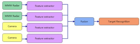
MMW radar and camera target-level fusion [25,26] means that the MMW radar and camera detect some of the features of the object separately, and then use a variety of algorithms and techniques to match and fuse the detected features, and finally to classify and process them, this fusion is mainly used for radar-aided imagery, and its principle is to use the radar to detect the target, generally detecting the middle of the object, as is shown in Figure 2, the detected target is projected on the image, a rectangular region of interest is generated empirically, and then this region is searched only to achieve joint calibration of the image and radar data.

The advantage of the method is that it can quickly exclude a large number of areas where there will be no targets, greatly increasing the speed of identification. Additionally, it can quickly exclude false targets detected by the radar, enhancing the reliability of the results. However, because of the inaccurate lateral distance to the target provided by the radar, combined with errors in camera calibration, the projection points of the MMW radar can deviate from the target more severely, and when the area of interest setting areas contains multiple targets, the targets are detected repeatedly, which can cause confusion in target matching.

Richter et al. [27] proposed a data processing method that combines radar observations with the results of contour-based image processing in 2008. Josip Ćesić and Marković et al. [28] extended the Kalman filter on the Lie group algorithm within the framework of modelling radar measurements and stereo camera measurements in polar coordinates as members of the Lie group and estimating the target state as the product of two special Euclidean motion groups for detecting and tracking moving data in 2016. Rong et al. [29] used MMW radar in the direction of vehicle-road cooperation to detect objects by reflected echoes, filtering the collected information for invalid signals and eliminating interference noise to identify the unique ID of the target as well as position and velocity information in 2020. This is spatially and temporally fused with the target feature information from the images identified by the camera.

In order to solve the data redundancy and errors of projecting radar data directly onto images. Du [30] proposed a 3D target detection algorithm in 2021, which first extracts image features from a single image while column expansion is performed on the radar point cloud, and then combines the 3D information output by the algorithm to match the corresponding radar point cloud columns. Radar features are constructed using the depth and velocity information of the radar; followed by fusion of the image features and radar features. An accurate 3D bounding box of the target is generated. In the same year, Nabati et al. [31] proposed an intermediate fusion method for 3D target detection using radar and camera data. A centroid detection network is first used to detect objects by identifying centroids on the image to obtain information such as 3D coordinates, depth, and rotation of the target. A new truncated cone based method is then used to correlate the radar detected data with the detected target centroids, and the features of the correlated target are concatenated with a feature map consisting of depth and velocity information detected by the radar data to complement the image features and return to target attributes such as depth, rotation, and velocity.

Decision-Level Integration

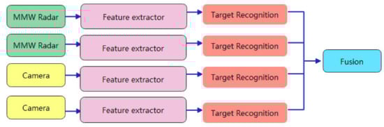
The decision level fusion of MMW radar data and camera data is a high level fusion. In this case, both the MMW radar and the camera have the ability to sense independently. The data detected by the MMW radar and the camera are first processed separately and both get an initial sensing result, and finally the image detection target results and the MMW radar detection results are effectively fused, which is shown in Figure 3. The advantages of this hierarchical fusion strategy are the flexibility in selecting sensor results, increased fault tolerance of the system, increased ability to accommodate multi-source heterogeneous sensors, improved real-time performance and smaller communication requirements in terms of bandwidth. However, the high level of information compression reduces accuracy and consumes too much pre-processing power. Commonly used fusion algorithms in the decision layer include Bayesian estimation, D-S evidence theory method.

Liu and Sparbert et al. [32] used MMW radar and camera sensors to generate a target decision separately and then combined their decisions to handle dynamic changes using interactive multi-model Kalman filtering, through a probabilistic data correlation scheme to achieve good object tracking. Amir Sole et al. [33] assume that both MMW radar and the camera can independently localise and identify interesting targets. In this case, when the radar target corresponds to the visual target, the target can be verified without further processing. When the radar target does not correspond to the visual target, several computational steps for non-matching radar target decisions are described in combination with direct motion parallax measurements and indirect motion analysis and pattern classification steps to cover cases where motion analysis is weakness or ineffective.

2.2. MMW Radars and Cameras Data Fusion Process

2.2.1. Spatial Fusion of MMW Radar and Vision Sensors

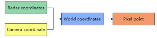
Spatial fusion of vision sensors and MMW radars is the conversion of acquired data from different sensors coordinate systems into the same coordinate systems. Cao et al. [34,35] investigated the spatial fusion technique of MMW radar and vision sensors. The millimetre wave radar coordinate system, camera coordinate system, pixel coordinate system, and world coordinate system between millimetre wave radar and visual sensor are researched as well as the transformation relationship between the various coordinate systems.

The world coordinate system, which is generally seen as a reference coordinate system for three-dimensional scenes, is an individually defined system of coordinates in three-dimensional space. In vision-related research, the world coordinate system is commonly used to describe the relationship between the transformation of an object’s position in three-dimensional space and other coordinate systems.

In this case, both the radar coordinate system and the camera coordinate system are defined by their mounting positions. The definition of the world coordinate system is artificial, some scholars define the radar coordinate system as the world coordinate system and some scholars define the camera coordinate as the world coordinate system. The main thought process is to first convert the MMW radar coordinate system to the camera coordinate system by rotation and translation, then from the camera coordinate system to the image coordinate system, and finally from the image coordinate system to the pixel coordinate system. The conversion of the coordinate system is therefore divided into three parts.

MMW Radar Coordinate System to Camera Coordinate System Conversion

The MMW radar coordinate system is converted to the camera coordinate system by rotation and translation, it is a three-dimensional-to-three-dimensional conversion. The conversion relationship between the two coordinates is shown in the following Equation (1)

$$\left[\begin{array}{c}{X}_C\\ Y_C\\ Z_C\\ 1\end{array}\right]=\left[\begin{array}{cccc}\cos \theta \cos \omega -\sin \theta \sin \omega \sin \psi & -\sin \theta \cos \psi & -\cos \theta \sin \omega +\sin \theta \sin \omega \sin \psi & X\\ \sin \theta \cos \omega -\sin \omega \sin \psi \cos \theta & \cos \theta \cos \psi & -\sin \theta \sin \omega +\cos \theta \cos \omega \sin \psi & Y\\ \sin \omega \cos \psi & -\sin \psi & \cos \omega \sin \psi & Z\\ 0& 0& 0& 1\end{array}\right]\left[\begin{array}{c}{X}_W\\ Y_W\\ Z_W\\ 1\end{array}\right]$$

(1)

The equation can be simplified as Equation (2)

$$\left[\begin{array}{c}{X}_C\\ Y_C\\ Z_C\\ 1\end{array}\right]=\left[\begin{array}{cc}R& T\\ 0^T& 1\end{array}\right]\left[\begin{array}{l}{X}_w\\ Y_w\\ Z_w\\ 1\end{array}\right]$$

(2)

In Equations (1) and (2), the radar coordinate system is ${(X}_W{,Y}_W,Z_W)$ and the coordinates of the corresponding point under the camera coordinate system is ${(X}_C{,Y}_C,Z_C)$. Where $\theta$ is the angle of rotation about $Z_W$ axis, $\psi$ is the angle of rotation about $X_W$ axis, $\omega$ is the angle of rotation about $Y_W$ axis, $X$ is the translation value $X_W$ along the axis, $Y$ is the translation value $Y_W$ along $Y_W$ axis, and $Z$ is the translation value $Z_W$ along $Z_W$ axis. $R$ is the rotation matrix, determined by the pitch and yaw angles of the camera, and $T$ is the translation array.

Conversion of Camera and Image Coordinate System

The camera coordinate system is converted from 3D to 2D by perspective projection onto the image coordinate system, the image coordinate system is in millimetres. According to the linear model of the camera, the camera coordinates are converted by similar triangles to obtain the image coordinate system. This is shown in the following Figure 4, and the point on the camera coordinates is converted to the coordinates on the image coordinate system as following Equation (3).

$$Z_C\left[\begin{array}{l}x\\ y\\ 1\end{array}\right]=\left[\begin{array}{cccc}f& 0& 0& 0\\ 0& f& 0& 0\\ 0& 0& 1& 0\end{array}\right]\left[\begin{array}{l}{X}_C\\ Y_C\\ Z_C\\ 1\end{array}\right]$$

(3)

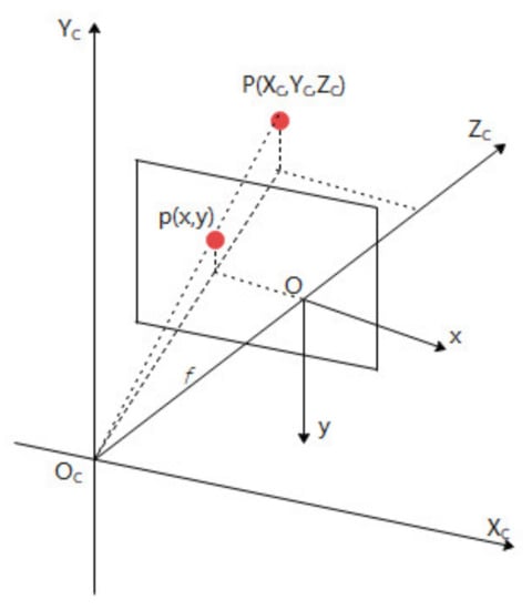
In Figure 4 and Equation (3), There is a point $P(X_C,Y_C,Z_C)$ in the camera coordinate system, the projection of the point $P$ in the image coordinate system of $xOy$ plane is $p(x,y)$, the intersection of the line between the point $P$ and $p$ the point and the optical lens is $O_C$, that is, the lens optical centre. The distance between the imaging plane and the optical lens is the focal length $f$ of the camera.

Conversion of Image and Pixel Coordinate Systems

The units of the pixel coordinate system are pixels, and the units of the image coordinate system are millimetres. The conversion is a two-dimensional-to-two-dimensional conversion, so the conversion of the coordinate system is a conversion of the origin as well as the units of measure. As is shown in Figure 5.

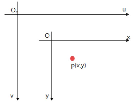
Where $O_O$ is the origin of the pixel coordinate system. The planes of $u{O}_{O}v$ coincide with the plane of $xOy$, and the u-axis is parallel to the x-axis, the v-axis is parallel to the y-axis. The pixel coordinates $(u,v)$ represent the pixel points located in the uth column and vth row of the image array. Thus, establishing the transformation equation for the above two coordinates yields the position of a point $(u,v)$ on the pixel coordinate system that lies on the image coordinate system.

The centre of the image coordinate system is theoretically $(u_0,v_0)$ located at the centre of the captured image, but due to camera manufacturing errors, the centres often do not overlap. Therefore, the equation for converting a point on the image coordinate system to a pixel coordinate system is shown in Equation (4).

$$\left[\begin{array}{c}u\\ v\\ 1\end{array}\right]=\left[\begin{array}{ccc}\frac{1}{dx}& 0& u_0\\ 0& \frac{1}{dy}& v_0\\ 0& 0& 1\end{array}\right]\left[\begin{array}{c}x\\ y\\ 1\end{array}\right]$$

(4)

where $(u_0,v_0)$ is the coordinates of the pixel coordinate system at the origin $O$, in the pixel coordinate system $dx$ and $dy$ are the width and height of each pixel, the point $(x,y)$ is the coordinate of point $p$ in the image coordinate system, and point $(u,v)$ is the coordinate of point $p$ in the pixel coordinate system.

In summary, combining and organising all the above equations completes the conversion equation from the MMW radar coordinate system to the camera coordinate system, to the image coordinate system and finally to the pixel coordinate system, as shown in the following Equation (5).

$$Z_C\left[\begin{array}{l}u\\ v\\ 1\end{array}\right]=\left[\begin{array}{ccc}\frac{1}{d_x}& 0& u_0\\ 0& \frac{1}{d_y}& v_0\\ 0& 0& 1\end{array}\right]\left[\begin{array}{cccc}f& 0& 0& 0\\ 0& f& 0& 0\\ 0& 0& 1& 0\end{array}\right]\left[\begin{array}{cc}R& T\\ 0^T& 1\end{array}\right]\left[\begin{array}{l}{X}_w\\ Y_w\\ Z_w\\ 1\end{array}\right]$$

(5)

The spatial fusion of the MMW radar and vision sensors is completed by converting the target detected by the MMW radar to the pixel coordinate system, and then converting the target detected by the camera to the pixel coordinate system, and then within the same pixel coordinate system, screening the target and correlating the front and back frame data to extract the target information. In addition to spatial fusion, the complete MMW radar and camera fusion technique also includes temporal fusion.

2.2.2. Camera Calibration

Camera calibration techniques mainly include the camera geometry model and the camera calibration method. The geometric model of the camera is used to find out the correspondence between the three-dimensional space and the two-dimensional space, and then the corresponding set of equations and constraints are established through the geometric model to solve the parameters, in turn, the image information can be reconstructed in three dimensions through the established geometric model, which is the calibration of the camera.

The internal parameters of the camera depend on the inherent internal structure of the camera and the external parameters of the camera depend on the information about the position of the camera. Ideally, the camera calibration model is a pinhole model, while in practice, the image captured by the camera will have some deviation from the actual image, which is caused by a certain degree of aberration in the camera’s lens due to processing, external forces and other factors. These include radial and centrifugal aberrations, thin lens aberrations and total aberrations. Therefore, when determining the internal and external parameters, the aberration parameters of the lens are also taken into account.

As the camera captures multiple pieces of information and each image contains a host of information, it is inefficient to process a whole image, so image features are extracted to process the points and areas of interest in the image. Image features are classified as edges, contours, textures, corner points, etc.

According to the conversion of the coordinate systems above, the internal and external parameters of the camera are used to obtain the specific values of the parameters according to the visual calibration of the camera. There are three types of camera calibration [36], including traditional camera calibration, camera self-calibration and active visual calibration methods.

Traditional Camera Calibration

Traditional camera calibration is based on a specific camera model and specific experimental conditions, the choice of size and size of the appropriate calibration reference, the use of a series of mathematical calculation methods, to find the camera internal and external parameters. The different types of physical calibration objects can be divided into three-dimensional physical calibration methods and flat-type physical calibration methods; the most common calibration objects are corner reflectors and Zhang’s board. The 3D calibration process is simple and can achieve good accuracy with only a single image, but the process and maintenance of the calibration object is more complex; flat type calibration cannot rely on a single image, it needs at least two images to support it, but the calibration object is simple to produce compared to 3D calibration object under the premise of ensuring calibration accuracy. The combined result is that the traditional camera calibration method cannot leave the support of the calibrator, and it cannot use or place the calibrator in certain specific environments, which has a large degree of scene limitation, and at the same time, the calibration effect is affected by the accuracy of the calibrator production. At present, the main calibration methods are as follows.

• Direct linear calibration method

The Direct Linear Transformation (DLT) method belongs to the typical traditional calibration, which can solve the calibration by direct linear transformation, it is first proposed by Aziz and Karara [37] in 1971, the Direct Linear Transformation method is an algorithm that directly establishes a linear relationship between the object position points in the three-dimensional world and the coordinate points in the image coordinate system. Since the DLT algorithm ignores the factor of lens distortion in imaging, it has the advantage of being a simple algorithm and easy to implement; the disadvantage is the lack of accuracy and large errors.

The image coordinate system and the camera coordinate system are transformed as follows Equation (6)

$$S\left[\begin{array}{l}x\\ y\\ 1\end{array}\right]={\mathrm{P}}_{3*4}\left[\begin{array}{l}{X}_C\\ Y_C\\ Z_C\\ 1\end{array}\right]$$

(6)

where $P$ is the projection factor and $S$ is the scale factor, then, eliminating $S$ Equation (6). After eliminating $S$, Equation (7) is obtained.

$$\begin{array}{l}{p}_{11}{X}_C+p_{12}{Y}_C+p_{13}{Z}_C+p_{14}-p_{31}x{X}_C-p_{32}x{Y}_C-p_{33}x{Z}_C-p_{34}x=0\\ p_{21}{X}_C+p_{22}{Y}_C+p_{23}{Z}_C+p_{14}-p_{31}x{X}_C-p_{32}x{Y}_C-p_{33}x{Z}_C-p_{34}x=0\end{array}$$

(7)

If there are $n$ points with coordinates in the world and image coordinate systems, respectively, then the system of linear equations containing the $2n$ equations, as shown in Equation (8).

$$H=AL=0$$

(8)

where $A$ is a (2Nx12) matrix and $L$ is the column vector of 11 dimensions, consisting of the elements of the projection matrix. The camera calibration is achieved by the process of finding the appropriate $L$ to makes the $\left|\right|H\left|\right|$ minimum.

2.

RAC two-step method

Tsai [38,39] established a RAC-based camera calibration algorithm in 1987, which uses the constraint of radial consistency to obtain some of the external parameters of the camera. As the method is often divided into two steps, it is also known as the RAC two-step method. The first step is to solve for some of the camera parameters using radial consistency, and the second step solves for the effective focal length, translational component, and aberration parameters of the camera. The advantage of the Tasi algorithm is its high accuracy, but the disadvantage is that it is complex and cumbersome to implement. Wu et al. [40] optimised the DLT algorithm by adding constraints on the transfer matrix through the RAC model to maintain the high real-time performance of the DLT algorithm itself and optimising the accuracy of the bit-pose computation of the DLT algorithm to improve the noise immunity and stability of the DLT algorithm.

In this method, the image coordinate system and the camera coordinate system are transformed as follows Equation (9).

$$\left[\begin{array}{l}x\\ y\\ 1\end{array}\right]=K[R|T]\left[\begin{array}{l}{X}_C\\ Y_C\\ Z_C\\ 1\end{array}\right]$$

(9)

Of which, $R=\left[\begin{array}{ccc}{r}_1& r_2& r_3\\ r_4& r_5& r_6\\ r_7& r_8& r_9\end{array}\right]$ and the $K=\left[\begin{array}{ccc}fs& 0& u_0\\ 0& f& v_0\\ 0& 0& 1\end{array}\right]$ according to Equation (9), Equation (10) is obtained by matrix transformation.

$$\left\{\begin{array}{c}x=\frac{fs(r_{1}X+r_{2}Y+r_{3}Z+t_1)}{r_{7}X+r_{8}Y+r_{9}Z+t_3}+u_0\\ y=\frac{s(r_{4}X+r_{5}Y+r_{6}Z+t_2)}{r_{7}X+r_{8}Y+r_{9}Z+t_3}+u_0\end{array}\right.$$

(10)

Transformation of ideal image coordinates to actual image coordinates considering only radial aberrations, like Equation (11).

$$\begin{array}{l}(x-u_c)(1+k_1(u^2+v^2))=u-u_c;\\ (y-v_c)(1+k_1(u^2+v^2))=v-v_c.\end{array}$$

(11)

In the first step, the rotation matrix $R$ and the translation matrix $T$ of the external parameters of the camera are found under the constraint of radial consistency; in the second step, the focal length $f$, the aberration parameter $k_1$ and the translation component $t_3$ in the z-axis direction of the camera are found by matrix transformation.

Using the resulting $f$, $t_3$ and $k_1=0$ as initial values, perform a nonlinear optimization of the following Equation (12).

$$\left\{\begin{array}{c}\frac{fs(r_{1}X+r_{2}Y+r_{3}Z+t_1)}{r_{7}X+r_{8}Y+r_{9}Z+t_3}(1+k_1(u^2+v^2))=u-u_0\\ \frac{s(r_{4}X+r_{5}Y+r_{6}Z+t_2)}{r_{7}X+r_{8}Y+r_{9}Z+t_3}(1+k_1(u^2+v^2))=v-v_0\end{array}\right.$$

(12)

Thus, the true value of $f$, $t_3$, $k_1$ is estimated, the internal and external parameters of the camera can be gained.

3.

Zhengyou Zhang plane calibration

In 1998, Zhang first proposed the Zhang’s planar calibration method [41]. This aimed at addressing changes in the internal and external parameters of the camera by solving the single-strain matrix. The calibration first requires the preparation of a template covered with a dot matrix and then uses the camera to take multiple photos from different directions. The single-strain matrix of each picture is calculated by the coordinates of the extracted feature points in the image coordinate system and their coordinates in the world coordinate system and is used to perform the camera calibration. The advantages of the Zhang’s calibration method are its easy template production, ease of use, low cost, robustness, and high accuracy. However, the process of the method is too complex and there is more manual interaction, which is not conducive to the improvement of automation. At present, the most widely used camera calibration is Zhang’s plane calibration.

According to Equation (12), assuming that the template is on a plane in $Z_C$ the world coordinate system, the following Equation (13) is obtained.

$$S\left[\begin{array}{l}x\\ y\\ 1\end{array}\right]=K[\begin{array}{ccc}{r}_1& r_2& r_3\end{array}]\left[\begin{array}{l}X\\ Y\\ 0\\ 1\end{array}\right]=K[\begin{array}{ccc}{r}_1& r_2& T\end{array}]\left[\begin{array}{l}X\\ Y\\ 0\end{array}\right]$$

(13)

where $K$ is the internal camera parameter matrix, $\left[\begin{array}{ccc}{r}_1& r_2& r_3\end{array}\right]$ is the rotation vector of the external camera parameters.

Let $M$ be the single strain matrix for each image, then we have Equation (14,15).

$$M=\left[\begin{array}{ccc}{h}_1& h_2& h_3\end{array}\right]=\lambda K\left[\begin{array}{ccc}{r}_1& r_2& T\end{array}\right]$$

(14)

$$r_1=\frac{1}{\lambda }{K}^{-1}{h}_1,r_2=\frac{1}{\lambda }{K}^{-1}{h}_2$$

(15)

According to the orthogonality of the rotation vectors, then we have Equation (16).

$$r_1^T{r}_2=0;\left|\right|r_1\left|\right|=\left|\right|r_2\left|\right|=1$$

(16)

Equation (17) can be obtained for each image.

$$\left\{\begin{array}{c}{h}_1^T{K}^{-T}{K}^{-1}{h}_2=0;\\ h_1^T{K}^{-T}{K}^{-1}{h}_1=h_2^T{K}^{-T}{K}^{-1}{h}_2.\end{array}\right.$$

(17)

There are five internal camera parameters, so when the number of images is greater than or equal to 3, then $K$ can be solved, then the external parameters and T for each image can be found from the single-strain matrix $M$ for each image.

Camera Self-Calibration

The camera self-calibration only uses the corresponding relationship among the images obtained by the camera in the process of movement and does not depend on any calibration reference in the calibration process, which is mainly due to the constraints of camera movement. The most commonly used are extinction point theorems (also known as vanishing point theorems), where parallel lines in space are represented as intersecting in the camera image plane. This calibration method is very flexible and allows for online calibration of the camera. The disadvantage is that it is based on absolute quadratic curves and surfaces, which are less robust and unrealistic for practical use. Currently, the main self-calibration methods [42] including self-calibration methods based on the Kruppa equation, self-calibration methods based on absolute quadratic surfaces, and infinity planes. Some scholars have also improved the existing methods.

Self-calibration based on absolute quadratic curves: Hartley and Faugeras et al. [43,44,45] introduced the concept of self-calibration in 1992. Through the idea of mapping geometry and according to the invariance of absolute quadratic curves, Faugeras obtains Kruppa equations, and the relevant internal parameters can be solved by solving the Kruppa equations. A series of refinements have since been developed [46,47], and the absolute quadratic curve is a special class of quadratic curve: a curve in the infinity plane that is strongly correlated with the geometric properties of Euclidean space. Moreover, the image of an absolute quadratic curve is only related to the camera’s internal reference and is independent of the camera’s motion and pose. Therefore, the constraints on the camera’s internal reference can be established by determining the position of the absolute quadratic curve in the image. Under the assumption that the internal reference of the camera is constant, the geometry of the pair of poles based on the absolute quadratic curve can be used to calibrate the internal parameters of the camera by solving the established Kruppa equation for a given three images.

The absolute quadratic surfaces are tangent to a plane of space to which an absolute quadratic curve is tangent is an absolute quadratic surface. The absolute quadric surface is the dual of the absolute quadratic curve. Similarly, the value of absolute quadric surface is only related to the internal parameters of the camera and irrelated to the motion of the camera. The camera calibration using absolute quadric surface is also based on this principle. In addition, the calibration method using absolute quadratic surfaces is more robust than the calibration method using absolute quadratic curves because it also contains information about the infinity plane. Before the camera is self-calibrated, it is assumed that the correspondence between images is deterministic and that the internal parameters of the camera do not change when different images are taken.

The preliminaries for the hierarchical stepwise calibration method [39] are the same as for the quadratic surface self-calibration method, which involves the radiometric reconstruction of a sequence of images and the Euclidean calibration, and then carry out the radiometric calibration and reconstruct the image sequence. Based on the photographic alignment of one image with all other images, which allows for a large reduction in the number of unknown parameters, while relying on a non-linear optimization algorithm to find all unknown quantities simultaneously. The disadvantage of such calibration methods is that the initial parameter values are ambiguous, and the photographic alignments are random, so different images are selected as references to obtain different camera parameter calibration results, resulting in uncertain convergence of the optimization algorithm. Xu et al. [48] proposed a new geometric method for camera self-calibration based on the fading point properties of two sets of opposite sides of a rectangle and the implied aspect ratio information. Using the property that the lines connecting finite-distance points in space to the same infinity point are parallel to each other and the harmonic partitioning of perfect quadrilaterals, as well as the feature that rectangles being imaged multiple times have the same aspect ratio, the constraint equations for the parameters within the camera are established. By establishing the cost function associated with the imaging of a linear segment, an aberration correction method is proposed that iterates between aberration parameter finding and linear internal parameter calibration to obtain a self-calibration accuracy comparable to that of the camera without aberrations. All external parameters of the camera can be solved by determining the coordinates of any two vertices of the rectangle.

Calibration methods using cooperative targets have been extensively investigated by scholars. Self-calibration is mainly accomplished using targets of prescribed shape, rectangular, linear, mathematical methods [49,50,51], or by using fading line features and can also be achieved by solving the uncalibrated camera n-point perspective (pnp) problem [52]. Due to the widespread availability of fading lines or fading points, the application of related methods is of high value. Existing methods for self-calibration using fading lines or fading points are mainly based on solving the fundamental matrix via circular points followed by a Cholesky decomposition to obtain the intra-camera parameter matrix.

Calibration Based on Active Vision

Active visual calibration method without relying on a calibrator, the camera is placed on a precisely controllable motion platform. The method uses known motion information to establish equations for the camera model parameters, which can usually be solved linearly and therefore has the advantages of ease of operation, high accuracy, and robustness, and is commonly used in active vision systems. It is only necessary to control the camera to make certain specific movements for which the motion information is known. However, the requirements for equipment and specific scenes are high, the equipment is expensive, the motion parameters are unknown, and the scenes are not controllable.

The linear method based on two sets of triple orthogonal motions, proposed by Ma [53] in 1996, is the best-known method for active visual calibration based on pure rotation of the camera [54]. Subsequently, Hu et al. have proposed calibration based on triple orthogonal translational motion and calibration based on a single strain matrix in the infinity plane [55], which can find one more parameter than Massaud’s method.

Hu and other active visual calibration method is based on the principle of orthogonal motion method of single response matrix in the plane [56], first assume that two vectors respectively are a set of orthogonal translation vectors to describe the camera motion information, according to these two vectors can get two corresponding single response matrix. Then it is possible to find the five internal parameters of the camera.

2.2.3. Combined MMW Radar and Camera Calibration

Traditional Joint Calibrations

The traditional joint space calibration of MMW radar and camera is to construct the radar coordinate system and camera coordinate system and establish the conversion function of the two coordinate systems, so that the target corresponds one by one in the radar coordinate system and image coordinate system. Traditional spatial transformation includes geometric projection principle and four points calibration method.

• Geometric projection

The calibration method of geometric projection converts a point from the radar coordinate system to a point in the world coordinate system, and then converts a point in the world coordinate system to the camera coordinate system i. The principle is shown in Figure 6. Conventional joint calibration also has some limitations, such as dependence on other sensors, low immunity to interference and distortion, and lack of self-calibration.

Gaoet al. [57] considered the non-linear distortion of the camera. Taking the non-linear distortion of the camera as the constraint condition, the coordinate transformation between radar correlation coordinates and camera correlation coordinates was introduced. After a characteristic transformation of the image-related coordinates to the radar-relative coordinates, a least-square method is used to determine the calibration parameters. Song [58] proposed a new method for the spatial calibration of a single camera and a two-dimensional radar. Using a marker, the position of the marker is measured simultaneously in the camera and radar coordinate systems. The marker position data is obtained by multiple measurements of the marker position. By aligning the points, the transformation between the radar coordinate system and the camera coordinate system is obtained and the accuracy of the marker is improved.

2.

Four-point calibration method

Guo et al. [59] proposed a four-point calibration method for the spatial synchronization of two sensors. On the basis of establishing the relationship between the coordinate systems of the two sensors, the method selects a 10 m area in front of the car as the calibration area, and uses two sets of point pairs on the ground in the area parallel to the radar centre axis to calibrate the horizontal angle of the vertical axis of the two sensor coordinate systems and the pitch angle of the camera. The improved four-point calibration method constructs a mapping function from the radar coordinate system to the camera coordinate system. It requires at least corresponding four pairs of points in the radar and camera coordinate systems, and the mapping function is easily obtained based on these four points. However, it is difficult to find the perfect four pairs of points for three reasons:

• The detection range of radar is generally larger than 100 m, so more points are needed to solve the mapping function;
• Any significant target in the camera image should occupy a certain area, so choosing a point in that area will create an error, and to reduce the error we need more pairs of points;
• If the devices are moved, they must be recalibrated.

Direct Calibration

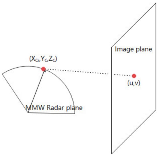
Shigeki et al. [20] first proposed the spatial calibration of radar and vision without calibrating the internal and external parameters of the camera, using the single-strain matrix and the reflection intensity of the radar. Based on this, Liu [60] proposed a single-strain-based method for calibrating Millimetre-wave radar data and CCD camera data. The method does not require manual operation for calibration. Wang et al. [61] proposed a single-strain point alignment method. An autonomous mobile vehicle experimental platform with radar and camera sensors was used to achieve point alignment between the MMW radar and the CCD camera. We assume that the radar is scanning and detecting on a flat surface, called the “MMW Radar plane”, as shown in Figure 7.

According to Equation (2), Equation (18) can be gained.

$$\omega \left[\begin{array}{c}u\\ v\\ 1\end{array}\right]=P\left[\begin{array}{c}{X}_C\\ Y_C\\ Z_C\\ 1\end{array}\right],P=\left[\begin{array}{cc}R& T\end{array}\right]$$

(18)

where $\omega$ is a constant. Considering that all the radar data comes from within the radar plane $(y=0)$, the above equation converts to Equation (19)

$$\omega \left[\begin{array}{c}u\\ v\\ 1\end{array}\right]=H\left[\begin{array}{c}{X}_C\\ Y_C\\ 1\end{array}\right]$$

(19)

where $H$ is a 3 × 3 single-strain matrix. Instead of estimating $R$ and $T$, the interconversion of the MMW radar plane and the camera plane can be achieved by simply asking for $H$. The joint calibration of the MMW radar and camera is completed.

Intelligent Calibration

Most traditional calibration methods involve the conversion of coordinates to the internal and external parameters of the camera, in recent years, a series of intelligent joint calibration methods have been proposed. The most obvious feature of intelligent calibration is that the joint calibration of MMW radar and camera can be achieved without converting coordinates.

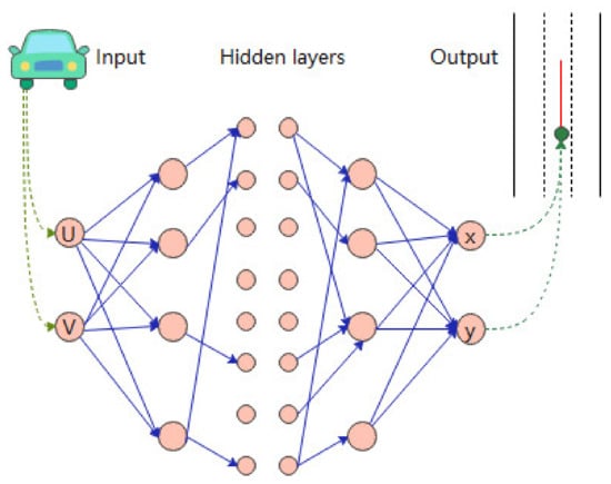
Liu [62] used online intelligent calibration to divide the road into three different areas, areas detectable only by cameras, areas detectable by both radar and cameras, and areas detectable only by radar, as shown in Equation (20).

$$\begin{array}{c}{P}^R=[X_{t1},X_{t2},\dots ,X_{tn}],X={[x,y]}^T\\ P^C=[U_{k1},U_{k2},\dots ,U_{kn}],U={[u,v]}^T\\ S^{RC}=\left[\left[\begin{array}{c}{X}_{t1}\\ U_{t1}\end{array}\right],\left[\begin{array}{c}{X}_{t1}\\ U_{t1}\end{array}\right]\dots \left[\begin{array}{c}{X}_{tj}\\ U_{tj}\end{array}\right]\right]\end{array}$$

(20)

where $P^R$ is the sequences monitored by radar, $P^C$ is the sequences monitored by the camera, and $S^{RC}$ is the joint monitoring sequence by the MMW radar and the camera. The neural network is then used to construct the mapping function. Both the input and output layers of the neural network contain two nodes. Finally the collected data are used to train and test the neural network iteratively. Special weighting is given to the online acquisition of data and the online training and testing of the neural network. Online intelligent spatial calibration is completed, as shown in Figure 8.

Gao et al. [63] used a curve fitting method for joint calibration of camera and MMW radar for objects, with the main vehicle was stationary, driving a target vehicle in the danger area from near to far, starting the camera vehicle recognition algorithm to identify the target vehicle, recording the image coordinates of the target vehicle detection centre and radar data information, removing the abnormal points in the data, and then using software to fit, and through experimental testing, the error is smaller and more robust than traditional joint calibration.

2.2.4. Temporal Fusion of MMW Radar and Vision Sensors

Due to the transmission frequency or sampling frequency of the MMW radar data processing and image data processing is different. The data collected by both the MMW radar and the camera are not at the same moment, resulting in a temporal bias in the data. The radar sampling frequency is generally lower than the video data. Therefore, it is necessary to detect objects dynamically in real time. Currently, there are two types of temporal fusion of MMW radar data and camera data, a hardware-based and a software-based synchronisation.

Hardware Synchronisation

Hardware synchronisation mainly involves setting up a hardware multi-thread trigger that triggers the camera to take a picture when the MMW radar captures the target information. Zhai et al. [64] used the camera data with low sampling frequency as a benchmark and used multi-thread synchronisation to achieve data time synchronisation. When each time the camera receives an image frame, the radar data corresponding to the current time of the image is acquired, as shown in Figure 9.

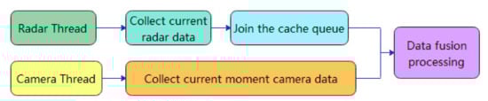
In order to achieve time synchronisation, a radar thread, a camera thread and a data fusion processing thread are created in the program. The radar thread is used to receive and process the radar data and the camera thread is used to receive and process the camera image data. When the data fusion processing thread is triggered, the system fetches the radar data in the radar data cache queue at the same moment as the image data for data fusion processing. The MMW radar and machine vision temporal fusion model. There is an initial time difference between the radar data and the image data due to the time difference between the moment of radar and camera activation, and this error is always less than the time it takes to refresh the radar data, so it does not affect the correctness of the time synchronisation.

Time synchronisation of multiple sensors mainly refers to processing data from sensors of different frequencies at the same moment. Qin [65] used a multi-threaded approach for time synchronisation, using QWaitCondition and QMutex in QT to achieve time synchronisation. The MMW radar data reception thread, the camera data reception thread and the main thread are set separately. Since the sampling frequency of the radar is lower than the sampling frequency of the camera, the sampling time node of the radar thread is used to trigger the sampling of the camera thread, the radar thread is always open, the camera data reception thread uses thread locking to keep it in a constant blocking state, and the camera data reception thread is triggered when the data reception of the radar data reception thread is completed. When the camera data receiving thread captures the image, the radar data receiving thread is closed. Through this method, the sensor data is captured at approximately the same moment, and the captured data is sent to the main thread for data processing, which runs in a loop to perform target detection, data correlation, and data output.

Software Synchronisation

At present, software synchronisation is the most commonly used solution, where a timestamp is added to the GPS. For example, MMW radar and camera acquired data have a GPS timestamp, then the data is compensated according to the nearest match or through interpolation methods, which are used in linear difference and Lagrangian interpolation.

Liu et al. [66] chose the Cubic Spline Interpolation to synchronize the information between sensors, if a sensor has checked $n$ times in a certain sampling period, its time point can be reduced to $(t_0,t_1,t_2,\dots t_n)$, let $f(t_i)$ as sensor’s measurement value of the $t_i$ moment, to satisfy $f(t_i)=y_i(i=1,2,\dots ,n)$ the combination of it into the fitting interpolation function $S(t)$. As the radar has a relatively stable sampling frequency, fixed at 20 Hz, and the camera sampling frequency varies according to the number of samples, this paper sets the frequency of the radar as the reference and establishes a Cubic Spline Interpolation function for the camera measurements, synchronising the radar and camera data in time.

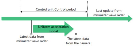
In order to make the data time synchronization of MMW radar and camera more accurate and fresher. Liu et al. [67] received the latest data of MMW radar in the current processing cycle of the control unit, and it is converted to the same timestamp as the most recent data from the camera using a uniform acceleration model The time synchronisation of the MMW radar and camera data is completed, as shown in Figure 10.

Ma et al. [68] used the camera data time as the standard to extrapolate the radar output to the target for the purpose of synchronisation with time. The specific implementation process is shown in Figure 11, where $T_r(n-2)$ and $T_r(n-1)$ are the timestamps of two consecutive radar data frames, $T_f(n)$ is the timestamp of the next data frame predicted by the radar tracking algorithm, with the same time difference between these three data frames.

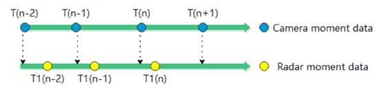
The position and velocity parameters of the radar target at $T_r(n-1)$ and $T_f(n)$ can be used to perform a linear interpolation operation to estimate the parameters of the radar target at the moment of $T_e(n)$, which can be expressed as Equation (21).

$$k=\frac{\Delta T_e(n)}{\Delta t}$$

(21)

2.2.5. MMW Radar and Image Data Information Correlation

An important component of the fusion of MMW radar data and camera data is data correlation, and the correctness of the data correlation is directly related to the effectiveness of the fusion. Therefore, the evaluation of information association algorithms and information correlation algorithms is also crucial.

IOU Discriminations

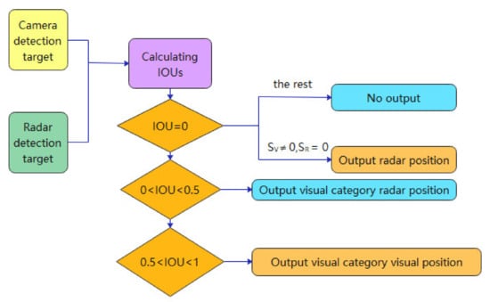
A typical decision-level information fusion approach [69] is to calculate the intersection ratio (IOU) of the detection frames obtained from the MMW radar and the camera for decision-level judgments. The IOU calculation equation is (22).

$$IOU=\frac{S_V\cap S_R}{S_V\cup S_R}$$

(22)

where $S_V$ is the depth vision detection rectangular frame area, $S_R$ is the MMW radar detection tracking rectangular frame area. When $IOU\in [0.5,1]$, output visual detection category and position information; when $IOU\in [0,0.5]$, output visual detection category with the target position and status information detected by the MMW radar; when $IOU=0$, no detection results are output, for $S_V\ne 0$ $S_R=0$ and $S_V\ne 0$, $S_R\ne 0$, $S_R\ne 0$ only the radar detection target position and status information is output when $S_V=0$, $S_R\ne 0$, until $IOU\ne 0$, as is shown in Figure 12.

Based on the Dichotomous Map Matching Principle

As the distance and velocity information given by the vision sensor is inaccurate and cannot be used directly for the final obstacle position and velocity output; meanwhile, the radar is characterised by a more accurate distance but lower resolution and poorer recognition performance, it needs to be matched with the radar clustering cluster using the position information from the matched radar as the output of the whole obstacle in order to achieve the complementary performance of the two sensors.

A data association algorithm based on the bipartite graph matching principle is proposed [70,71,72], mainly for solving the case of incorrect matching caused by a relatively large error in one of the sensors.

Use the set $X=\left\{\left.x_1,x_2,x_3,\dots x_m\right\}\right.$ to represent the full set of visual obstructions, and additionally use the set $Y=\left\{\left.y_1,y_2,y_3,\dots x_n\right\}\right.$ to represent the full set of radar clusters, through abstracting the full set into a bipartite graph $G=〈X,E,Y〉$ where the edges of $E$ is $〈x,y〉$ which represent that visual obstacle; it $x$ can be matched to the $y$.

Qin [66] proposed an algorithm for target association in 3D space, where both MMW radar and camera can provide relative distance information of the target, and co-associate the distance information of both with the coordinate information of the centroid in the image, defining the cost function as $f$, when $f$ the minimum is determined that the target in the MMW radar sequence and the target in the camera sequence are the same target. Then we have Equation (23).

$$f=w_u\left|u_c-u_r\right|+w_v\left|v_c-v_r\right|+w_{dist}\left|d_c-d_r\right|$$

(23)

where $u_c$ is the horizontal coordinate of the pixel coordinate system of the centre point of the vehicle detected by the camera, $v_c$ is the vertical coordinate of the pixel coordinate system of the centre point of the vehicle detected by the camera; $u_r$ is the horizontal coordinate of the pixel coordinate system of the centre point of the vehicle detected by the radar, $v_r$ is the vertical coordinate of the pixel coordinate system of the centre point of the vehicle detected by the radar.

Lastly, $d_c,d_r$ are the distances detected by the camera and the radar for the vehicle ahead, respectively.

Typical Data Association Algorithms

• Joint Probabilistic Data Association (JPDA)

The JPDA [73,74,75] is one of the data association algorithms corresponding to the case where observations fall into the intersection region of a tracking gate, which may originate from multiple targets. The JPDA aims to calculate the probability of association between the observations and each target and considers that all valid echoes may originate from each particular target, only the probability that they originate from different targets. The advantage of the JPDA algorithm is that it can track and recognize multiple targets without being affected by clutter. However, when the number of targets and measurements increases, the JPDA algorithm will experience a combinatorial explosion in computational effort, which results in computational complexity. After acquiring the target sequence, Sun et al. [76] introduced the Marxian distance for observation matching based on the target-level fusion method. Then the JPDA was applied for data fusion to establish the system observation model and state model, thus realizing the target recognition based on information fusion.

2.

Multiple Hypothesis Tracking (MHT)

MHT [77,78,79,80] is another algorithm for data association. Unlike JPDA, the MHT algorithm retains all hypotheses of the real target and lets them continue to be passed, then to remove the uncertainty of the current scan cycle from the subsequent observations. Under ideal conditions, MHT is the optimal algorithm for handling data correlation, it can detect the end of a target and the generation of a new target. However, when the clutter density increases, the computational complexity increases exponentially, and it is also difficult to achieve target-measurement pairing in practice.

2.3. MMW Radar and Camera Information Fusion Algorithm

2.3.1. Traditional Information Fusion Algorithms

Weighted Average Method

Weighted averaging method is the process of matching the target results from each sensor and then weighting the results according to the weights accounted for by each MMW radar and camera sensor, with the weighted average being used as the result of the fusion. If the signal from one sensor is more plausible than the others, a higher weight is assigned to that sensor to increase its contribution to the fused signal.

Advantage: it is the simplest and most straightforward method, practically efficient and has a code-easy to implement approach to real-time information processing fusion methods.

Disadvantage: This method is more suitable for dynamic environments but requires detailed analysis of sensor results and performance to obtain accurate weights.

Chen [81] used radar depth-of-field information to acquire regions of interest quickly and with high accuracy. The unification of time and space in radar and camera was accomplished through the ADTF software platform, and the acquisition of data was completed by selecting a weighted average information fusion algorithm to fuse the MMW radar and camera information. According to the advantages of the two sensors, Xu et al. [82] used a fusion method including, longitudinal distance using only the detection results of the MMW radar, lateral distance using the detection results of the camera and MMW radar weighted by the camera, the camera accounted for a larger proportion of the target type using only the classification results of the camera. Wang et al. [83] used a weighted averaging algorithm to fuse the MMW radar and camera data, putting a certain sensor will reduce the weight to 0 when the target is judged to be non-normal by its own marker position or target location, it will not participate in the fusion at the non-normal point, in order to avoid accidental errors substantially reducing the post-fusion accuracy at this point.

Least Squares Method

The Least squares method is the approximate fitting of target observations from different sensors that the sum of squares of the errors in the fitting function for the target observations from different sensors is minimised. The Least squares method is generally not used alone but is used together with other fusion methods, or to verify the quality of other fusion methods. The least squares method is needed to fit points and compare the functions to minimise the sum of squares of the errors for each point to obtain the final coefficients. The resulting curve is then the fused trajectory points.

Kalman Filtering Algorithm and Its Variants

The Kalman filtering algorithm can be divided into standard Kalman filtering [84], interval Kalman filtering [85] and two-stage Kalman filtering [86]. The method uses recursion of the statistical properties of the measurement model to determine the optimal fusion and data estimation in a statistical sense. If the system has a linear dynamics model and the system-sensor error fits a Gaussian white noise model, the Kalman filter will provide the only statistically significant optimal estimate of the fused data. MMW radar and camera fusion is a smooth stochastic process, which has a linear dynamic model and the system noise conforms to a Gaussian distributed white noise model and is sensitive to error information, hence a number of studies have been carried out by many experts and scholars.

Kalman filtering is mainly used to fuse low-level real-time dynamic multi-sensor redundant data, where the data received by the sensors generally has a large error when fused at the pixel level. The Kalman filtering method can effectively reduce the error between the data and thus improve the fusion effect.

Advantage: the system processes without the need for powerful data storage and computing power and is suitable for fusion between different levels of raw data with little loss of information.

Disadvantages: a need to build an accurate model of the observed object, the data requirements are also large, and the scope of application is relatively narrow. With a large amount of redundancy in the combined information, the amount of computation will increase dramatically by three times the filter dimension which is difficult to meet in real-time. The increase in sensor subsystems increases the probability of failure, and in the event of a failure in one system that is not detected in time, the failure can contaminate the entire system, making it less reliable.

Liu et al. [87] designed a traffic flow data acquisition system based on the radar and vision camera. In order to make the vehicle operation data measured by the sensor more accurate, the optimal estimation algorithm based on Kalman filter can be used to optimally estimate the vehicle transverse and longitudinal speed, acceleration, and head-to-tail spacing measured by the radar and vision camera, which improves the measurement accuracy. Liu [88] pre-processed the collected camera and MMW radar raw data to obtain the target data from the camera and MMW radar, and then judged whether the camera and MMW radar detected the target, when both detected the target at the same time, firstly Kalman filtering was performed, secondly through the strong tracking Kalman filter algorithm STF (Strong Tracking Filter) fusion algorithm processing to obtain more accurate target information, when one of the sensors detects a target, the data detected by the corresponding sensor is output, and when neither sensor detects a target, there is no target in the area, thus completing the target detection based on data fusion and storing it.

Lu [89] designed and developed a Kalman filter module, a Munkres matching algorithm module and other fusion aid modules using the global nearest neighbour idea. Wu et al. [90] used distributed sensor fusion to carry out target tracking research using Kalman filtering. Amditis [91] proposed a new Kalman filter-based method with a measurement space that includes data from radar and vision systems, which is robust during vehicle manoeuvres and turns.

Cluster Analysis

After obtaining the agreement of the individual MMW radar and camera data, it is easy to cluster the data points based on the agreement, which collect similar points. The formula for agreement shows that points with a distance less than a threshold have a high degree of agreement, and points with a large distance have a low degree of agreement. Typical clustering analysis algorithms include Marxian distance, Euclidean distance, and global nearest neighbour (GNN) [92,93].

The clustering presupposes is to discuss consistency, where cluster analysis fuses data with a high degree of consistency, and individual data that are ‘inconsistent’ may be considered to be ‘singularities’ caused by chance under adverse circumstances. If a cluster analysis appears as multiple classes that are distantly distributed, then the overall data is highly inconsistent and reflects different system characteristics that cannot be simply fused.

Consistency is a potential function $K(X,Y)$ which requires several conditions to be satisfied:

• The output of the function is between 0 and 1, when the two points $X$, $Y$ are very close to the output value, when the two points are very far away to the output value is small;
• A progressive decline in the trend of the function;
• When the two points $X$, $Y$ coincide (distance is 0), the output is 1, when the distance between the two points is infinite, the output is 0;
• $K(X,Y)=K(Y,X)$ is a continuous function.

Typical cluster analysis refers to the Marxist distance [94] and is widely used in the fusion detection process of MMW radar and cameras [95,96]. The martingale distance is a method proposed by Indian statisticians to calculate the covariance distance between two points. The Marcian distance between the predicted and observed values is defined as Equation (24)

$$d_M=\sqrt{{(z_i-z_{k|k-1})}^T{S}_k^{-1}(z_i-z_{k|k-1})}$$

(24)

where $Z_i$ is the ith target observation of the current cycle; $Z_{k|k-1}$ is the target prediction of the current cycle based on the previous $k-1$ moments; and $S_k^{-1}$ is the covariance matrix between the two samples, whose mth row and nth column elements are defined as the covariance of the mth and nth elements of the two samples. In [77], the method acquires the target sequence and then introduces the Marcian distance for matching the observations. Thus, information fusion-based target recognition is achieved.

In the past few decades, various experts and scholars have applied GNN algorithms to MMW radar and camera data fusion well; Zhang et al. [97] used the target detection intersection and ratio and GNN data association algorithm to achieve multiple MMW radar and camera sensor data fusion, which selected the association scheme with the lowest total cost after comprehensive consideration of the overall association cost, which is more in line with the actual working conditions, and less computationally intensive. Liu [66] and Jia [98] used the GNN to match the vehicle information data collected by MMW radar and camera with the target source.

Fuzzy Theory

Fuzzy theory [99,100] is based on human thinking patterns, and the basic idea is to use machines to simulate human control of the system, according to the unified characteristics of the cognition of objective things, it summarizes, extracts, abstracts and summarizes, and finally evolves into fuzzy rules to help the corresponding function make the result judgment. Fuzzy theory can work with different algorithms depending on the specific situation to solve the problem of uncertainty. Currently, fuzzy theory is widely used in MMW radar and camera fusion technology. Firstly, based on fuzzy logic, the data collected by each sensor is fuzzified and transformed into a fuzzy concept that represents the characteristics of the object; then, the processed data is evaluated in a comprehensive manner to determine the state of the current environment. Its main applications are the processing of MMW radar data and image data [101,102,103].

Strengths: using a linguistic approach, precise mathematical models of the process are not required, the system is robust and can solve non-linear problems in the fusion process. It can adapt to changes in the dynamics of the monitored object, changes in environmental characteristics and changes in operational conditions, and is highly fault tolerant. The operator can easily communicate with the human-machine interface through natural human language.

Disadvantages: the fuzzy processing of the original data will lead to lower control accuracy and poorer dynamic quality of the system. The design of fuzzy control still lacks systematicity and cannot define the control objectives. In the feature layer, suitable algorithms need to be selected contacted the actual situation and combined with fuzzy theory to make them work together effectively to improve the melting effect. However, the difficulty of fuzzy theory lies in how to construct reasonable rules for judging indicators and affiliation functions.

Neural Network-Based Algorithms

The neural network-based algorithm is a method that has been established in recent years based on the continuous development and maturity of neural network technology. It makes use of the properties of neural networks and can better solve the error problem of sensor systems. The basic information processing unit of a neural network is the neuron. Using different forms of connections between neurons and choosing different functions, different learning rules and final results can be obtained. This enriches the diversity of fusion algorithms. Furthermore, differences in the chosen learning databases lead to different effects in the fusion results. There are good results in the processing of radar data and in the association of two sensors data [104,105].

Bayesian Approach

The Bayesian approach is to treat each sensor as a Bayesian estimate. Liu et al. [106] used a Bayesian formulation to calculate the state estimate of the target to obtain suboptimal solutions, for the radar and camera, and subsequently combined the local estimates of the sensors in a distributed fusion structure to obtain global estimates. Cou [107] obtained good data correlation based on Bayesian programming for multi-sensor data fusion of LIDAR, MMW radar, and camera.

D-S Method

Evidence-theoretic algorithm, also known as the Dempster-Shafer algorithm, or the D-S algorithm [108]. This method is an expansion of Bayesian inference and can be used for decision inference using a statistically based data fusion algorithm, evidence theory, when the verdict derived from multiple MMW radar and camera information is not 100% confident. The algorithm can fuse the knowledge acquired by multiple sensors and finally find the intersection of the respective knowledge and the corresponding probability assignment value. A wide range of applications are available for multi-sensor fusion.

D-S algorithm includes three basic points: basic probability assignment function, trust function and likelihood function. The inference structure of the D-S method is from top to bottom which is divided into three levels: the first level is goal synthesis, where data information from multiple sensors is pre-processed to calculate the basic probability distribution function, confidence, and release of each piece of evidence; the second level is inference, where the basic probability distribution function, confidence, and release of all the data from the same sensor are calculated according to the D-S synthesis rules. The third level is updating, where each sensor is generally subject to random error, so that a set of consecutive reports (reports are the processed probability distribution function, credibility, release, etc.) from the same sensor sufficiently independently in time is more reliable than any single report. Thus, the observations from the sensors are combined (updated) before inference and multi-sensor synthesis.

Advantage: the a priori data is more intuitive and easier to obtain than in probabilistic inference theory. D-S formula can synthesise knowledge or data from different experts or data sources, and it makes evidence theory widely used in areas such as expert systems and information fusion. Areas of application of the algorithm include information fusion, expert systems, intelligence analysis, legal case analysis, multi-attribute decision analysis, etc.

Disadvantage: requires the evidence to be independent, a condition that is sometimes not easily met. In addition, the evidence synthesis rule does not have solid theoretical support, and its soundness and validity are still highly controversial. The theory of evidence suffers from a potential exponential explosion in computation.

The block diagram of MMW radar and CCD camera information fusion, proposed by Luo et al. [109], based on the D-S evidence method is shown in Figure 13. Firstly, the identification framework is established, then the basic probability distribution function of each evidence is calculated for the information obtained from each sensor and the basic probability distribution function under the combined action of all the evidence is calculated according to the combination rules of the D-S evidence method, and finally according to the given judgment criterion the hypothesis with the highest confidence level is selected as the fusion result.

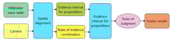
The confidence function based on different evidence on the same recognition frame of the MMW radar and CCD camera is given as the confidence function resulting from their joint action. This function is a sum of their confidence functions. Let ml (Xi) and mc (Xi) functions as the confidence functions on the same recognition frame for the MMW radar and the CCD camera, respectively. The fusion results of the MMW radar and the CCD camera are obtained according to Dempster’s rule.

Jin et al. [110] used the D-S algorithm to fuse the data features after MMW radar and camera feature extraction for detecting the safety of night-time driving. Converting the world coordinates of the radar target to image coordinates, forming a region of interest on the image, using image processing methods to reduce interference points, and applying D-S evidence theory to fuse feature information to obtain a total confidence value to examine vehicles in the region of interest. Liu et al. [111] obtained from four typical maritime obstacle scenarios 3D LIDAR, MMW radar and stereo vision perception data, and each grid is assigned a corresponding weight according to the detection accuracy of different sensors in different perception areas. Integration of grid attributes using D-S combination rules This results in a fused USV obstacle representation.

Each of the above traditional information fusion algorithms is not only limited to use alone, but scholars have also used a mixture of each algorithm in order to expect the best MMW radar and camera information fusion results. For example, in the literature [68] used algorithms such as Kalman filtering and weighted fusion to achieve 1R1V (1 Radar 1 Vision) sensory information fusion.

2.3.2. Deep Learning Based on Information Fusion Algorithms

Deep Learning, also known as Deep Neural Network, is the result of continuous research and development of artificial neural networks. Through decades of experience, it has become clear that the expressive power of neural network systems tends to increase as the number of implicit layers increases, allowing them to perform more complex classification tasks and to approximate more complex mathematical function models. The features or information obtained after the network model has been ‘learned’ are then stored in a distributed connection matrix, and the ‘learned’ neural network is then capable of feature extraction, learning and knowledge memory. Due to the more significant ‘intelligence’ of deep learning, there have been many scholars attempts to apply it to MMW radar and camera fusion algorithms to improve the accuracy of multi-sensor data fusion.

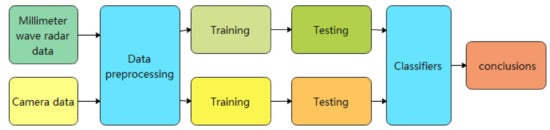
In the data fusion process of MMW radar and camera, deep learning is mainly used for feature extraction of camera features before fusion, and Mon [112] proposed a vehicle front target detection and recognition method. The method performs target detection and recognition of the obtained visual information through the deep learning algorithm which is named YOLO-v2, and then further improves the reliability of target detection by processing, analysing, and projecting the MMW radar data and correlating the radar point cloud data and images in the fusion process sheet, as well as testing and training the fused data after the fusion. Wang et al. [113] mapped the MMW radar detected forward obstacle information onto the image to form regions of interest in the image, each region of interest was passed to a nested cascaded Adaboost classifier to detect whether the forward obstacle was a vehicle. Zhang et al. [114] used the wraparound box regression algorithm to analysis.

CNN-Based Multi-Sensor Data Fusion Model

Currently, Convolutional Neural Network (CNN) is one of the most important methods in the field of intelligent image and video processing. Convolutional operations are the most important operations in CNN. The features extracted are theoretically invariant to image translation, rotation and scaling, and have two features of local perception and weight sharing, which makes the CNN more closely resemble the perceptual properties of real creatures and reduces a large number of weight learning parameters compared to global connections.

CNN can be seen as a combination of feature extraction and classifier, from the mapping of each layer, it is similar to extracting features at different levels. Neural networks are highly fault tolerant and can be used in complex non-linear mapping environments. The strong fault tolerance and the self-learning, self-organising and self-adaptive capabilities of neural networks meet the requirements of multi-sensor data fusion technology processing. Neural networks determine the classification criteria in the data model primarily based on the similarity of the samples accepted by the current system, a process characterised as the distribution of weights in the network. The signal processing capabilities and automatic inference functions of neural networks can achieve multi-sensor data fusion. As is shown in Figure 14.

Traditional neural networks map images layer by layer and then extracts the features in it. Currently, CNN are mostly used for fusion. Some scholars [63,115] used Kalman filtering to process radar data, generate regions of interest in the images, and detect vehicles in the regions by an improved deep vehicle recognition algorithm. Jiang [116] used an information fusion association algorithm to determine the association between the radar and the ROI region detected by machine vision: if the two ROI regions are successfully associated, the same target is considered to be detected and the output is used as the final detection target. If the association fails, the ROI region that failed to be associated is detected again using an Adaboost classifier. After the fusion of MMW radar and vision to obtain the region of interest of the image, Wu [117] used CNN to identify the image to determine whether there was a person or a car in the ROI region to achieve the predefined target of MMW radar for verification and achieve the fusion of MMW radar and vision in terms of information. Lekic and Babic [118] proposed a fully unsupervised machine learning algorithm for fusing radar sensor measurements and camera images in 2019.

The spatial information grid modelling of radar sensor data of evidence, and the whole set of occupancy state estimation is called grid layer. By combining the network layer and camera image into the network, under the condition of radar data, multiple network generate image like camera, so as to realize the feature fusion of radar and camera data. This contains all the environmental features detected by the radar sensors. The algorithm converts the radar sensor data into an artificial, camera-like image of the environment. Through this data fusion, the algorithm produces information that is more consistent, accurate and useful than that provided by radar or cameras alone.

The convolutional neural network, proposed by Kim et al. [119], uses a modified VGG16 model and a feature pyramid network two-stage architecture, combined with radar and image feature representation, to provide good accuracy and robustness for target detection and localization.

Meyer [120] used manually labelled bounding boxes to train deep convolutional neural networks to detect vehicles. The results show that deep learning is often a suitable method for target detection from radar data.

Chadwick [121] designed and trained a detector that operates using monocular images and radar scans to perform robust vehicle detection in a variety of settings. The overall framework uses the SSD algorithm to include radar data using image features, and the use of a branching structure also provides the potential flexibility of using weights from different radar representations of the RGB branches. As with standard SSD, features at different scales are convolved by classification and regression to produce dense predictions on a predefined default set of boxes.

Lim [122] proposed a new deep learning architecture fusing radar signals and camera images, in which the radar and camera branches are tested, trained, and extracted separately.

DLSTM-Based Data Fusion Model

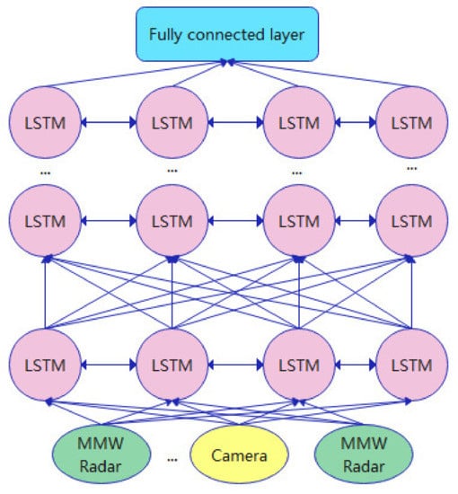
The structure of the Deep Long Short Time Memory (DLSTM) data fusion prediction model [123,124], as is shown in Figure 15. The prediction accuracy and reliability can be improved by using multiple sensor data as compared to single sensor data. Multiple LSTM layers are stacked to form a DLSTM model to fuse multi-sensor data and extract deep features, with different LSTM layers connected spatially and data input from upper layer neurons to lower layer neurons, with information exchanged between the LSTM neurons in each LSTM layer.

Advantages: deep neural networks that have a powerful non-linear representation ability which enables them to fully explore the deep abstract features between multiple sources of data, avoiding the problem of reducing the accuracy of model output due to insufficient feature extraction; deep learning has self-learning ability, which enables them to obtain the correlation between multiple sources of information on their own and fully fuse them according to the correlation; data fusion methods based on deep learning have good real-time performance when running on equipment with strong computing power which can meet the real-time requirements in related fields. Deep learning-based data fusion methods have good real-time performance when running on devices with strong computing power and can meet the real-time requirements of related fields. Therefore, deep learning-based data fusion methods have better performance compared to traditional data fusion methods.

Disadvantages: the characteristics of deep learning models also limit their application to a certain extent. Currently, most deep learning algorithms increase the depth and network complexity of the model in order to improve the non-linear representation of the network, but they also increase the parameters of the model and the difficulty of training the model, and further increase the consumption of computing resources. Therefore, deep learning-based data fusion methods are not applicable in small devices such as sensor network nodes and removable terminals.

3. Results

This paper reviews the key techniques of MMW radar and camera fusion, including the definition, layers, and structures of MMW radar and camera fusion, and reviews the advantages and disadvantages of each layer and structure. Since the fusion of MMW radar and camera involves only two different sensors, more distributed fusion structures are used, and since MMW radar generates a large number of false targets and invalid data, more scholars choose to fuse pairs at the feature layer. The MMW radar and camera fusion process is briefly described, including spatial and temporal fusion, and the widely used calibration method in spatial fusion is “Zhang” calibration, as well as some new online intelligent calibration methods. Online intelligent calibration methods can achieve rapid calibration to a certain extent on different websites, but the accuracy of calibration and the stability of calibration system cannot be guaranteed. In the future, we need to improve the traditional calibration, and research and develop a more stable online calibration system. Finally, the algorithms for information fusion are described, where deep learning based on fusion algorithms achieve faster speeds and better data correlation than traditional fusion algorithms and may become mainstream in the near future. However, deep learning still has its limitations, including large amount of calculation, high hardware requirements, complex model design, and inability to judge the right or wrong of low-level data. In future development, it would be very important to overcome the difficulties of deep learning in fusion with two complementary sensors, due to the low accuracy of MMW radar and camera fusion. Thus, MMW radar and camera fusion are not widely used. Discovering an appropriate fusion algorithm to realize its fusion would be very important.

At present in the field of transportation, the fusion of MMW radar and camera is mostly used for vehicle automatic driving and assisted driving. With the development of intelligent transportation, the fusion technology of MMW radar and camera can be gradually used on the intelligent roadside. Through the acquisition, analysis, and application of roadside data, traffic conflicts would be effectively reduced and vehicle road coordination would be realized. Some high-speed highways in China have begun to use MMW radars and cameras on the roadside. In the future, according to the good properties of these devices, more roads will use these two sensors to make traffic more intelligent.

The technology of MMW radar and camera fusion will be a research field with rapid technology update frequency and various blooming industries.

References

- Wei, W.B.; Rui, X.T.; Chen, Y.S. Study on millimeter wave radar homing head. Tactical Missile Technol. 2008, 24, 83–87. [Google Scholar]
- Hou, W.G. Key Technologies for UAV-Borne Millimeter-Wave Broadband Obstacle Avoidance Radar Based on FPGA. Master’s Thesis, Nanjing University of Science and Technology, Nanjing, China, 2017. [Google Scholar]
- Van der Sanden, J.J.; Short, N.H. Radar satellites measure ice cover displacements induced by moving vehicles. Cold Reg. Sci. Technol. 2017, 133, 56–62. [Google Scholar] [CrossRef]
- Signore, R.; Grazioso, S.; Fariello, A.; Murgia, F.; Selvaggioc, M.; Gironimo, G. Conceptual design and control strategy of a robotic cell for precision assembly in radar antenna systems. Procedia Manuf. 2017, 11, 397–404. [Google Scholar] [CrossRef]
- Gouveia, C.; Tomé, A.; Barros, F.; Soares, S.; Vieira, J.; Pinho, P. Study on the usage feasibility of continuous-wave radar for emotion recognition. J. Biomed. Signal Processing Control. 2020, 58, 101835. [Google Scholar] [CrossRef]
- Han, C.; Han, L.; Sun, L.; Guo, J. Millimeter wave radar gesture recognition algorithm based on spatio-temporal compressed feature representation learning. J. Electron. Inf. 2022, 44, 1274–1283. [Google Scholar]
- Javaid, M.; Haleem, A.; Singh, R.P.; Rab, S.; Suman, R. Exploring impact and features of machine vision for progressive industry 4.0 culture. J. Sens. Int. 2022, 3, 100132. [Google Scholar] [CrossRef]
- Bellocchio, E.; Crocetti, F.; Costante, G.; Fravolini, M.L.; Valigi, P. A novel vision-based weakly supervised framework for autonomous yield estimation in agricultural applications. J. Eng. Appl. Artif. Intell. 2022, 109, 104615. [Google Scholar] [CrossRef]
- Bowman, A.N. Executing a vision for regenerative medicine: A career beyond the bench. Dev. Biol. 2020, 459, 36–38. [Google Scholar] [CrossRef]
- Huang, S.L.; Zhang, J.X.; Bu, Z.F. Literature review of military applications of machine vision technology. Ordnance Ind. Autom. 2019, 2, 2. [Google Scholar]
- Da Silva Santos, K.R.; Villani, E.; de Oliveira, W.R.; Dttman, A. Comparison of visual servoing technologies for robotized aerospace structural assembly and inspection. Robot. Comput.-Integr. Manuf. 2022, 73, 102237. [Google Scholar] [CrossRef]
- Du, C.F.; Jiang, S.B. Application of computer vision and perception in intelligent security. J. Telecommun. Sci. 2021, 37, 142–147. [Google Scholar]
- Xia, Y.Q.; Kang, J.O.; Gan, Y.; Jin, B.H.; Qian, S.Y. Review of intelligent transportation system based on computer vision. J. Zhengzhou Inst. Light Ind. Nat. Sci. Ed. 2014, 29, 52–60. [Google Scholar]
- Wang, B.F.; Qi, Z.Q.; Ma, G.C.; Cheng, S.Z. Vehicle detection based on information fusion of radar and machine vision. J. Automot. Eng. 2015, 37, 674–678. [Google Scholar]
- Alessandretti, G.; Broggi, A.; Cerri, P. Vehicle and guard rail detection using radar and vision data fusion. IEEE Trans. Intell. Transp. Syst. 2007, 8, 95–105. [Google Scholar] [CrossRef] [Green Version]
- Zhao, L. Multi-sensor information fusion technology and its applications. Infrared 2021, 42, 21. [Google Scholar]
- Grover, R.; Brooker, G.; Durrant-Whyte, H.F. A low level fusion of millimeter wave radar and night-vision imaging for enhanced characterization of a cluttered environment. In Proceedings of the 2001 Australian Conference on Robotics and Automation, Sydney, Australia, 30 March–1 April 2001. [Google Scholar]
- Steux, B.; Laurgeau, C.; Salesse, L.; Wautier, D. Fade: A vehicle detection and tracking system featuring monocular color vision and radar data fusion. In Proceedings of the Intelligent Vehicle Symposium 2002, Versailles, France, 17–21 June 2002; Volume 2, pp. 632–639. [Google Scholar]
- Fang, Y.; Masaki, I.; Horn, B. Depth-based target segmentation for intelligent vehicles: Fusion of radar and binocular stereo. IEEE Trans. Intell. Transp. Syst. 2002, 3, 196–202. [Google Scholar] [CrossRef]
- Sugimoto, S.; Tateda, H.; Takahashi, H.; Okutomi, M. Obstacle detection using millimeter-wave radar and its visualization on image sequence. In Proceedings of the ICPR 2004, Cambridge, UK, 26 August 2004; Volume 3, pp. 342–345. [Google Scholar]
- Wu, S.G.; Decker, S.; Chang, P.; Camus, T.; Eledath, J. Collision sensing by stereo vision and radar sensor fusion. IEEE Trans. Intell. Transp. Syst. 2009, 10, 606–614. [Google Scholar]
- Wang, T.; Zheng, N.N.; Xin, J.; Ma, Z. Integrating millimeter wave radar with a monocular vision sensor for on-road obstacle detection applications. Sensors 2011, 11, 8992–9008. [Google Scholar] [CrossRef] [Green Version]
- Chavez-Garcia, R.O.; Burlet, J.; Vu, T.D.; Aycard, O. Frontal object perception using radar and mono-vision. In Proceedings of the 2012 IEEE Intelligent Vehicles Symposium, Madrid, Spain, 3–7 June 2012; pp. 159–164. [Google Scholar]
- Ji, Z.; Prokhorov, D. Radar-vision fusion for object classification. In Proceedings of the 2008, 11th International Conference on Information Fusion, Cologne, Germany, 30 June–3 July 2008; pp. 1–7. [Google Scholar]
- Steinberg, A.N.; Bowman, C.L. Rethinking the JDL data fusion levels. Nssdf Jhapl 2004, 38, 39. [Google Scholar]
- He, Y.; Guan, X.; Wang, G.H. Progress and prospects of multi-sensor information fusion research. J. Astronaut. 2005, 26, 524–530. [Google Scholar]
- Richter, E.; Schubert, R.; Wanielik, G. Radar and vision based data fusion-advanced filtering techniques for a multi object vehicle tracking system. In Proceedings of the 2008 IEEE Intelligent Vehicles Symposium, Eindhoven, The Netherlands, 4–6 June 2008; pp. 120–125. [Google Scholar]
- Ćesić, J.; Marković, I.; Cvišić, I.; Petrović, I. Radar and stereo vision fusion for multitarget tracking on the special Euclidean group. Robot. Auton. Syst. 2016, 83, 338–348. [Google Scholar] [CrossRef]
- Rong, S.H.; Wang, S.H.; She, H.Y. Application of millimeter wave radar and video fusion in vehicle-road cooperation system. In Proceedings of the 15th Annual China Intelligent Transportation Conference, Shenzhen, China, 4–7 November 2020; pp. 181–189. [Google Scholar]
- Du, X. Research on the Algorithm of Vehicle Front Target Detection Based on Millimeter Wave Radar and Visual Information Fusion. Master’s Thesis, Chongqing University of Technology, Chongqing, China, 2021. [Google Scholar] [CrossRef]
- Nabati, R.; Qi, H. Centerfusion: Center-based radar and camera fusion for 3d object detection. In Proceedings of the IEEE/CVF Winter Conference on Applications of Computer Vision, Waikoloa, HI, USA, 3–8 January 2021; pp. 1527–1536. [Google Scholar]
- Liu, F.; Sparbert, J.; Stiller, C. IMMPDA vehicle tracking system using asynchronous sensor fusion of radar and vision. In Proceedings of the 2008 IEEE Intelligent Vehicles Symposium, Eindhoven, The Netherlands, 4–6 June 2008; pp. 168–173. [Google Scholar]
- Sole, A.; Mano, O.; Stein, G.P.; Kumon, H.; Tamatsu, Y.; Shashua, A. Solid or not solid: Vision for radar target validation. In Proceedings of the IEEE Intelligent Vehicles Symposium, Parma, Italy, 14–17 June 2004; pp. 819–824. [Google Scholar]
- Cao, C.; Gao, J.; Liu, Y.C. Research on space fusion method of millimeter wave radar and vision sensor. Procedia Comput. Sci. 2020, 166, 68–72. [Google Scholar] [CrossRef]
- Li, X. Forward vehicle information recognition based on millimeter wave radar and camera fusion. Master’s Thesis, Chang’an University, Xi’an, China, 2020. [Google Scholar] [CrossRef]
- Xiao, Y.J.; Huang, C.H.; Zhang, T. A review of camera calibration techniques. Commun. World Half Mon. 2015, 7, 206–207. [Google Scholar]
- Abdel-Aziz, Y.; Karara, H.M. Direct linear transformation into object space coordinates in close-range photogrammetry. In Proceedings of the Symposium on Close-Range Photogrammetry; University of Illinois: Urbana, IL, USA, 1971; pp. 1–18. [Google Scholar]
- Tsai, R. A versatile camera calibration technique for high-accuracy 3D machine vision metrology using off-the-shelf TV cameras and lenses. IEEE J. Robot. Autom. 1987, 3, 323–344. [Google Scholar] [CrossRef] [Green Version]
- Sun, P. Research on the Calibration Method of Camera; Northeast Petroleum University: Heilongjiang, China, 2016. [Google Scholar]
- Wu, J.M.; Li, Y.F.; Chen, N.N.; Wu, L. An improved DLT camera pose estimation method using RAC model. J. Southwest Univ. Sci. Technol. 2019, 34, 71. [Google Scholar]
- Zhang, Z.Y. A new camera calibration technique based on circular points. IEEE Trans. Pattern Anal. Mach. Intell. 2000, 22, 1330–1336. [Google Scholar] [CrossRef] [Green Version]
- Shu, N. Research on Camera Calibration Methods; Nanjing University of Technology: Nanjing, China, 2014. [Google Scholar]
- Maybank, S.J.; Faugeras, O.D. A theory of self-calibration of a moving camera. Int. J. Comput. Vis. 1992, 8, 123–151. [Google Scholar] [CrossRef]
- Luong, Q.T.; Faugeras, O.D. Self-calibration of a moving camera from point correspondences and fundamental matrices. Int. J. Comput. Vis. 1997, 22, 261–289. [Google Scholar] [CrossRef]
- Lourakis, M.I.A.; Deriche, R. Camera Self-Calibration Using the Singular Value Decomposition of the Fundamental Matrix: From Point Correspondences to 3D Measurements; INRIA: Paris, France, 1999. [Google Scholar]
- Huang, T.S.; Faugeras, O.D. Some properties of the E matrix in two-view motion estimation. IEEE Trans. Pattern Anal. Mach. Intell. 1989, 11, 1310–1312. [Google Scholar] [CrossRef]
- Mendonça, P.R.S.; Cipolla, R. A simple technique for self-calibration. In Proceedings of the 1999 IEEE Computer Society Conference on Computer Vision and Pattern Recognition (Cat. No PR00149), Fort Collins, CO, USA, 23–25 June 1999; Volume 1, pp. 500–505. [Google Scholar]
- Xu, S.; Sun, X.X.; Liu, X.; Cai, M. A rectangle-based geometric method for self-calibration of cameras. J. Opt. 2014, 2014, 225–238. [Google Scholar]
- Wu, F.; Wa, G.; Hu, Z. A linear approach for determining intrinsic parameters and pose of cameras from rectangles. J. Softw. 2003, 14, 703–712. [Google Scholar]
- Wang, R.; Li, X.; Zhang, G. A linear algorithm for determining intrinsic parameters of zoomed monocular camera in the vision based landing of an UAV. Acta Aeronaut. Astronaut. Sin.-Ser. A B 2006, 27, 676. [Google Scholar]
- Olver, P.J.; Tannenbaum, A. Mathematical Methods in Computer Vision; Springer Science & Business Media: Berlin, Germany, 2003. [Google Scholar]
- Guo, Y.; Zhang, X.D.; Xu, X.H. An analytic solution for the noncoplanar P 4 P problem with an uncalibrated camera. Chin. J. Comput. 2011, 34, 748–754. [Google Scholar] [CrossRef]
- Songde, M. A self-calibration technique for active vision system. IEEE Trans. Robot. Autom. 1996, 12, 114–120. [Google Scholar]
- Hartley, R.I. Self-calibration of stationary cameras. Int. J. Comput. Vis. 1997, 22, 5–23. [Google Scholar] [CrossRef]
- Wu, F.C.; Hu, Z. A new theory and algorithm of linear camera self calibration. Chin. J. Comput. Chin. Ed. 2001, 24, 1121–1135. [Google Scholar]
- Li, H.; Wu, F. Chao. A new method for self-calibration of linear cameras. J. Comput. Sci. 2000, 23, 1121–1129. [Google Scholar]
- Gao, D.; Duan, J.; Yang, X.; Zheng, B.G. A method of spatial calibration for camera and radar. In Proceedings of the 8th World Congress on Intelligent Control and Automation, Jinan, China, 7–9 July 2010; pp. 6211–6215. [Google Scholar]
- Song, C.; Son, G.; Kim, H.; Gu, D.; Lee, J.H.; Kim, Y. A novel method of spatial calibration for camera and 2D radar based on registration. In Proceedings of the 6th IIAI International Congress on Advanced Applied Informatics (IIAI-AAI), Hamamatsu, Japan, 9–13 July 2017; pp. 1055–1056. [Google Scholar]
- Guo, L.; Liu, Z.F.; Wang, J.Q.; Li, K.Q.; Lian, X.M. A spatial synchronization method for radar and machine vision. J. Tsinghua Univ. Nat. Sci. Ed. 2006, 46, 1904–1907. [Google Scholar]
- Liu, X.; Cai, Z. Advanced obstacles detection and tracking by fusing millimeter wave radar and image sensor data. In Proceedings of the ICCAS, Gyeonggi-do, Korea, 27–30 October 2010; pp. 1115–1120. [Google Scholar]
- Wang, T.; Xin, J.; Zheng, N. A method integrating human visual attention and consciousness of radar and vision fusion for autonomous vehicle navigation. In Proceedings of the 2011 IEEE Fourth International Conference on Space Mission Challenges for Information Technology, Palo Alto, CA, USA, 2–4 August 2011; pp. 192–197. [Google Scholar]
- Liu, M.; Li, D.; Li, Q.K.; Lu, W. An online intelligent method to calibrate radar and camera sensors for data fusing. J. Phys. Conf. Ser. 2020, 1631, 012183. [Google Scholar] [CrossRef]
- Gao, J.D.; Jiao, X.; Liu, Q.Z. Machine vision and millimeter wave radar information fusion for vehicle detection. China Test. 2021, 9, 22. [Google Scholar]
- Zhai, G.Y.; Chen, R.; Zhang, J.F.; Zhang, J.G.; Wu, C.; Wang, Y.M. Obstacle detection based on millimeter wave radar and machine vision information fusion. J. Internet Things 2017, 1, 76–83. [Google Scholar]
- Qin, H. Research on Forward Vehicle Detection Algorithm Based on Vision and Millimeter Wave Radar Fusion. Hunan University: Changsha, China, 2019. [Google Scholar] [CrossRef]
- Liu, C.; Zhang, G.L.; Qiu, H.M. Research on target tracking method based on multi-sensor fusion. J. Chongqing Univ. Technol. 2021, 35, 1–7. [Google Scholar]
- Liu, T.; Zhu, Z.; Guan, H. Research on some key issues based on 1R1V sensing information fusion. Automot. Compon. 2021, 22, 22–25. [Google Scholar] [CrossRef]
- Ma, Z.G.; Zheng, Y. A sensor-based target track initiation decision algorithm for camera and millimeter wave radar fusion systems. Shanghai Automot. 2020, 17, 4–8. [Google Scholar]
- Gan, Y.D.; Zheng, L.; Zhang, Z.D.; Li, Y.N. Fusion of millimeter wave radar and depth vision for multi-target detection and tracking. Automot. Eng. 2021, 43, 1022–1029. [Google Scholar]
- Huang, Y. Research and Application of Obstacle Detection Algorithm by Fusing Camera and Millimeter Wave Radar; Yangzhou University: Yangzhou, China, 2020. [Google Scholar] [CrossRef]
- Wei, E.W.; Li, W.H.; Zhang, Z.H.; Zheng, J. A non-intrusive load matching method based on improved Hungarian algorithm. Electr. Meas. Instrum. 2019, 56, 58–64. [Google Scholar]
- Wang, P. 2-Factors in bipartite graphs containing perfect pair sets. J. Math. Phys. 2004, 24, 475–479. [Google Scholar]
- Liu, J.; Liu, Y.; He, Y.; Sun, S. A joint probabilistic data interconnection algorithm based on all-neighborhood fuzzy clustering in a cluttered wave environment. J. Electron. Inf. 2016, 38, 1438–1445. [Google Scholar]
- Zhang, J.; Xiong, W.; He, Y. Performance analysis of several simplified joint probabilistic data interconnection algorithms. Syst. Eng. Electron. Technol. 2005, 27, 1807–1810. [Google Scholar]
- Luo, S.Q.; Chen, X.; Wu, Q.; Zhou, Z.; Yu, S. Hfel: Joint edge association and resource allocation for cost-efficient hierarchical federated edge learning. IEEE Trans. Wirel. Commun. 2020, 19, 6535–6548. [Google Scholar] [CrossRef]
- Sun, N.; Qin, H.M.; Zhang, L.; Ge, R.H. Vehicle target recognition method based on multi-sensor information fusion. Automot. Eng. 2017, 39, 1310–1315. [Google Scholar]
- He, J.Z.; Wu, C.; Zhou, Z.; Cheng, S.F. A review of multi-hypothesis tracking techniques. Firepower Command. Control. 2004, 29, 1–5. [Google Scholar]
- Streit, R.L.; Luginbuhl, T.E. Probabilistic Multi-Hypothesis Tracking; Naval Underwater Systems Center: Newport, RI, USA, 1995. [Google Scholar]
- Gong, H.; Sim, J.; Likhachev, M.; Shi, J. Multi-hypothesis motion planning for visual object tracking. In Proceedings of the 2011 International Conference on Computer Vision, Barcelona, Spain, 6–13 November 2011; pp. 619–626. [Google Scholar]
- Zhai, H. Research on multi-hypothesis tracking algorithm and its application. Inf. Technol. Res. 2010, 18, 25–27. [Google Scholar]
- Chen, X. Development of Radar and Vision Information Fusion Algorithm for Vehicle Recognition in Front of Cars; Jilin University: Changchun, China, 2016. [Google Scholar]
- Xu, W.; Zhou, P.Y.; Zhang, F.; Huang, L. Vision and millimeter wave radar information fusion algorithm for pedestrian recognition. J. Tongji Univ. 2017, 45, 37–42+91. [Google Scholar]
- Wang, Y.Y.; Liu, Z.G.; Deng, H.Y.; Xu, Z.X.; Pan, D. Automatic lane-changing environment sensing system for electric trolleys. J. Tongji Univ. 2019, 47, 1201–1206. [Google Scholar]
- Chui, C.K.; Chen, G. Kalman Filtering; Springer International Publishing: Berlin/Heidelberg, Germany, 2017. [Google Scholar]
- Motwani, A.; Sharma, S.K.; Sutton, R.; Culverhouse, P. Interval Kalman filtering in navigation system design for an uninhabited surface vehicle. J. Navig. 2013, 66, 639–652. [Google Scholar] [CrossRef] [Green Version]
- Zhang, J.H.; Welch, G.; Bishop, G.; Huang, Z.Y. A two-stage Kalman filter approach for robust and real-time power system state estimation. IEEE Trans. Sustain. Energy 2013, 5, 629–636. [Google Scholar] [CrossRef]
- Liu, Y.H.; Zhang, Y.; Liu, G.P.; Zhang, H.K.; Jin, L.L.; Fan, Z.D. Design of a traffic flow data collection system based on Ravision. Comput. Meas. Control. 2022, 22, 1929. [Google Scholar]
- Liu, Y. Research on Multi-Sensor-Based Vehicle Environment Sensing Technology; Changchun University of Technology: Changchun, China, 2020. [Google Scholar]
- Lu, Y. Development of 1R1V-based sensor fusion algorithm. China Integr. Circuit 2020, 29, 66–71. [Google Scholar]
- Wu, X.; Wu, Y.; Shao, J. Research on target tracking based on millimeter wave radar and camera fusion. Mechatronics 2018, 24, 3–9+40. [Google Scholar]
- Amditis, A.; Polychronopoulos, A.; Floudas, N.; Andreone, L. Fusion of infrared vision and radar for estimating the lateral dynamics of obstacles. Inf. Fusion 2005, 6, 129–141. [Google Scholar] [CrossRef]
- Wu, X.; Ren, J.; Wu, Y. Study on target tracking based on vision and radar sensor fusion. SAE Techn. Paper 2018, 2018, 1–7. [Google Scholar] [CrossRef]
- Gong, P.; Wang, C.; Zhang, L. Mmpoint-GNN: Graph neural network with dynamic edges for human activity recognition through a millimeter-wave radar. In Proceedings of the 2021 International Joint Conference on Neural Networks (IJCNN), Shenzhen, China, 18–22 July 2021; pp. 1–7. [Google Scholar]
- McLachlan, G.J. Mahalanobis distance. Resonance 1999, 4, 20–26. [Google Scholar] [CrossRef]
- Milella, A.; Reina, G.; Underwood, J. A self-learning framework for statistical ground classification using radar and monocular vision. J. Field Robot. 2015, 32, 20–41. [Google Scholar] [CrossRef]
- Milella, A.; Reina, G.; Underwood, J.; Douillard, B. Combining radar and vision for self-supervised ground segmentation in outdoor environments. In Proceedings of the 2011 IEEE/RSJ International Conference on Intelligent Robots and Systems, San Francisco, CA, USA, 25–30 September 2011; pp. 255–260. [Google Scholar]
- Zhang, B.L.; Zhan, Y.H.; Pan, D.W.; Chen, J.; Song, W.J.; Liu, W.T. Vehicle detection based on millimeter wave radar and machine vision fusion. Automot. Eng. 2021, 43, 478–484. [Google Scholar]
- Jia, W. Research on Vehicle Detection Method Based on Radar and Vision Fusion; Dalian University of Technology: Dalian, China, 2021. [Google Scholar]
- Leondes, C.T. Fuzzy Theory Systems; Academic Press: Cambridge, MA, USA, 1999. [Google Scholar]
- Zimmermann, H.J. Fuzzy set theory. Wiley Interdiscip. Rev. Comput. Stat. 2010, 2, 317–332. [Google Scholar] [CrossRef]
- Boyd, R.V.; Glass, C.E. Interpreting ground-penetrating radar images using object-oriented, neural, fuzzy, and genetic processing//Ground Sensing. Int. Soc. Opt. Photonics 1993, 1941, 169–180. [Google Scholar]
- Cheng, Z.M.; Liu, X.L.; Qiu, T.Y. Vehicle target recognition system based on fuzzy control for millimeter wave radar. In Proceedings of the 9th International Conference on Intelligent Human-Machine Systems and Cybernetics (IHMSC), Hangzhou, China, 26–27 August 2017; Volume 1, pp. 175–178. [Google Scholar]
- Choi, B.; Kim, B.; Kim, E.; Lee, H.; Yang, K.W. A new target recognition scheme using 24GHz microwave RADAR. In Proceedings of the 2012 International conference on Fuzzy Theory and Its Applications (iFUZZY2012), Taichung, Taiwan, 16–18 November 2012; pp. 220–222. [Google Scholar]
- Cennamo, A.; Kaestner, F.; Kummert, A. A neural network based system for efficient semantic segmentation of radar point clouds. Neural Processing Lett. 2021, 53, 3217–3235. [Google Scholar] [CrossRef]
- Winter, M.; Favier, G. A neural network for data association. In Proceedings of the IEEE International Conference on Acoustics, Speech, and Signal Processing, Phoenix, AZ, USA, 12–17 May 1999; Volume 2, pp. 1041–1044. [Google Scholar]
- Liu, C.; Zhang, G.L.; Zheng, Y.W.; He, X.Y. A multi-sensor fusion method based on detection of trace-free information fusion algorithm. Automot. Eng. 2020, 42, 854–859. [Google Scholar]
- Coué, C.; Fraichard, T.; Bessiere, P.; Mazer, E. Multi-sensor data fusion using Bayesian programming: An automotive application. Intelligent Vehicle Symposium: Versailles, France, 2002; Volume 2, pp. 442–447. [Google Scholar]
- Dai, Y.P.; Ma, J.J.; Ma, X.H. Theory and Application of Intelligent Fusion of Multi-Sensor Data; Mechanical Industry Press: Beijing, China, 2021; pp. 119–140. [Google Scholar]
- Luo, Y.; Lei, Y.; Wang, I. A DS fusion method based on millimeter wave radar and CCD camera information. Data Acquis. Processing 2014, 29, 648–653. [Google Scholar]
- Jin, L.S.; Cheng, L.; Cheng, B. Detection of vehicles ahead at night based on millimeter wave radar and machine vision. J. Automot. Saf. Energy Conserv. 2016, 7, 1354. [Google Scholar]
- Liu, D.; Zhang, J.; Jin, J.; Dai, Y.S.; Li, L.G. A new approach of obstacle fusion detection for unmanned surface vehicles using Dempster-Shafer evidence theory. Appl. Ocean. Res. 2022, 119, 103016. [Google Scholar] [CrossRef]
- Mo, C. Research on Environment Perception Algorithm of Intelligent Vehicle Based on Vision and Radar Information Fusion; Chongqing University: Chongqing, China, 2018. [Google Scholar]
- Wang, S.; Zhang, R. Vehicle detection based on millimeter wave radar and vision information fusion. Sci. Technol. Wind. 2019, 7. [Google Scholar] [CrossRef]
- Zhang, X.; Zhou, M.; Qiu, P.; Huang, Y.; Li, J. Radar and vision fusion for the real-time obstacle detection and identification. Ind. Robot. Int. J. Robot. Res. Appl. 2019, 46, 391–395. [Google Scholar] [CrossRef]
- Shi, Y.; Li, J. Sensor fusion technology in the field of automotive autonomous driving. Equip. Mach. 2021, 21, 2140. [Google Scholar]
- Jiang, Y. Research on Forward Vehicle Detection and Tracking Algorithm with Millimeter Wave Radar and Machine Vision Fusion; Chongqing University: Chongqing, China, 2019. [Google Scholar] [CrossRef]
- Wu, S.J. Research on millimeter wave radar and vision fusion boarding bridge forward target recognition method. Univ. Electron. Sci. Technol. 2021. [Google Scholar] [CrossRef]
- Lekic, V.; Babic, Z. Automotive radar and camera fusion using generative adversarial networks. Comput. Vis. Image Underst. 2019, 184, 1–8. [Google Scholar] [CrossRef]
- Kim, J.; Kim, Y.; Kum, D. Low-level sensor fusion network for 3D vehicle detection using radar range-azimuth heatmap and monocular image. In Proceedings of the Asian Conference on Computer Vision, Kyoto, Japan, 30 November–4 December 2020. [Google Scholar]
- Meyer, M. Deep learning based 3D object detection for automotive radar and camera. In Proceedings of the European Radar Conference, Paris, France, 2–4 October 2019. [Google Scholar]
- Chadwick, S.; Maddern, W.; Newman, P. Distant vehicle detection using radar and vision. In Proceedings of the International Conference on Robotics and Automation (ICRA), Montreal, Canada, 20–24 May 2019; pp. 8311–8317. [Google Scholar]
- Lim, T.Y.; Ansari, A.; Major, B.; Fontijne, D.; Hamilton, M.; Gowaikar, R.; Subramanian, S. Radar and camera early fusion for vehicle detection in advanced driver assistance systems. In Proceedings of the Machine Learning for Autonomous Driving Workshop at the 33rd Conference on Neural Information Processing Systems, Vancouver, Canada, 8–14 December 2019; p. 2. [Google Scholar]
- Zhang, H.; Cheng, C.; Xu, Z.; Li, J. A review of research on data fusion methods based on deep learning. Comput. Eng. Appl. 2020, 24, 1–11. [Google Scholar]
- Wu, J.; Hu, K.; Cheng, Y.W.; Zhu, H.P.; Shao, X.Y.; Wang, Y.H. Data-driven remaining useful life prediction via multiple sensor signals and deep long short-term memory neural network. ISA Trans. 2019, 97, 241–250. [Google Scholar] [CrossRef]
Publisher’s Note: MDPI stays neutral with regard to jurisdictional claims in published maps and institutional affiliations. |
© 2022 by the authors. Licensee MDPI, Basel, Switzerland. This article is an open access article distributed under the terms and conditions of the Creative Commons Attribution (CC BY) license (https://creativecommons.org/licenses/by/4.0/).