CO₂Flux Model Assessment and Comparison between an Airborne Hyperspectral Sensor and Orbital Multispectral Imagery in Southern Amazonia

Abstract

In environmental research, remote sensing techniques are mostly based on orbital data, which are characterized by limited acquisition and often poor spectral and spatial resolutions in relation to suborbital sensors. This reflects on carbon patterns, where orbital remote sensing bears devoted sensor systems for CO₂ monitoring, even though carbon observations are performed with natural resources systems, such as Landsat, supported by spectral models such as CO₂Flux adapted to multispectral imagery. Based on the considerations above, we have compared the CO₂Flux model by using four different imagery systems (Landsat 8, PlanetScope, Sentinel-2, and AisaFenix) in the northern part of the state of Mato Grosso, southern Brazilian Amazonia. The study area covers three different land uses, which are primary tropical forest, bare soil, and pasture. After the atmospheric correction and radiometric calibration, the scenes were resampled to 30 m of spatial resolution, seeking for a parametrized comparison of CO₂Flux, as well as NDVI (Normalized Difference Vegetation Index) and PRI (Photochemical Reflectance Index). The results obtained here suggest that PlanetScope, MSI/Sentinel-2, OLI/Landsat-8, and AisaFENIX can be similarly scaled, that is, the data variability along a heterogeneous scene in evergreen tropical forest is similar. We highlight that the spatial-temporal dynamics of rainfall seasonality relation to CO₂ emission and uptake should be assessed in future research. Our results provide a better understanding on how the merge and/or combination of different airborne and orbital datasets that can provide reliable estimates of carbon emission and absorption within different terrestrial ecosystems in southern Amazonia.

1. Introduction

Global warming, population growth, and the gradual increase in greenhouse gas concentrations have been the subject of several studies using remote sensing (RS) techniques [1,2,3,4,5]. RS has a critical role in understanding different environmental concerns, especially those related to land use and land cover changes (LULCC).

Extremely useful and common in LULCC research, orbital remote sensing data are characterized by limited acquisition since they are collected in a specific time interval, in addition to the presence of clouds, which cover the surface, causing missing data problems in optical datasets [6,7]. Moreover, most orbital sensors are multispectral, which usually means poorer spectral resolution compared to suborbital sensors and, therefore, data restraint [8].

Orbital remote sensing bears devoted sensor systems for CO₂ monitoring and assess different scenarios, for instance, quantifying power plants emission [9,10], urban emissions [11], wildfire emissions [12] and the related measure of solar-induced chlorophyll fluorescence [13,14]. However, recurrent observation systems as Landsat [15], Sentinel-2 [16] and PlanetScope [17] provide reasonable data for modelling or assessing CO₂ dynamics [18]. Meanwhile, remote sensing based on airborne sensors are present on carbon cycle research [19,20], where promising applications are emerging with LIDAR in measuring soil organic carbon (SOC) [21], as well as with aboveground biomass [22,23].

The CO₂Flux emission model [24] aims to parameterizes the photosynthetic flux, originally of boreal forests, using the light use efficiency (LUE) concept. In turn, LUE is related to the fraction of photosynthetically active radiation absorbed by green biomass (fAPAR), i.e., canopy photosynthetic capacity [25,26,27].

Understanding the CO₂Flux emission depends on the associated indices relying on two spectral models. On one hand, the Normalized Difference Vegetation Index (NDVI) expresses the presence or the absence of vegetation and, when it comes to vegetation, the type (e.g., forest, soybean, pasture) and its greenness [28]. On the other hand, the Photochemical Reflectance Index (PRI) is related to light use efficiency (LUE) of photosynthetically active vegetation (that is, in the visible spectral range) based on hyperspectral data from AVIRIS [29,30]. Assuming multispectral imagery, PRI and its scaled version (sPRI) data have higher correlation to LUE using MODIS band 13 (662–672 nm), using backscattered images [31].

As mentioned above, the applicability of the CO₂Flux emission model [19] is based on hyperspectral data of AVIRIS (Airborne Visible/Infrared Imaging Spectrometer), which qualifies the airborne sensor Specim^® AisaFENIX [32] for this type of study. This airborne dataset (in forestry research) has low temporal resolution and availability, impeding the progress in terms of assessing the CO₂ emission and uptake with this dataset. We also highlight that CO₂ surveys are characterized by requiring tuned models to different types of ecosystems [33].

Although the CO₂Flux model [24] has been mainly used with hyperspectral data, several studies have assessed the application of PRI to multispectral imagery by using this vegetation index (VI) with blue and green bands, substituting the bands at 531 nm and 570 nm, respectively [16,34,35,36,37,38,39,40]. It is also important to mention that drought condition affect PRI results in CO₂Flux estimation [41].

Based on the considerations above, we have compared the CO₂Flux model by using four different imagery systems (Landsat 8, PlanetScope, Sentinel, AisaFenix) in the northern part of the state of Mato Grosso, southern Brazilian Amazonia. The study area covers three different land uses, which are primary tropical forest, bare soil, and pasture.

2. Materials and Methods

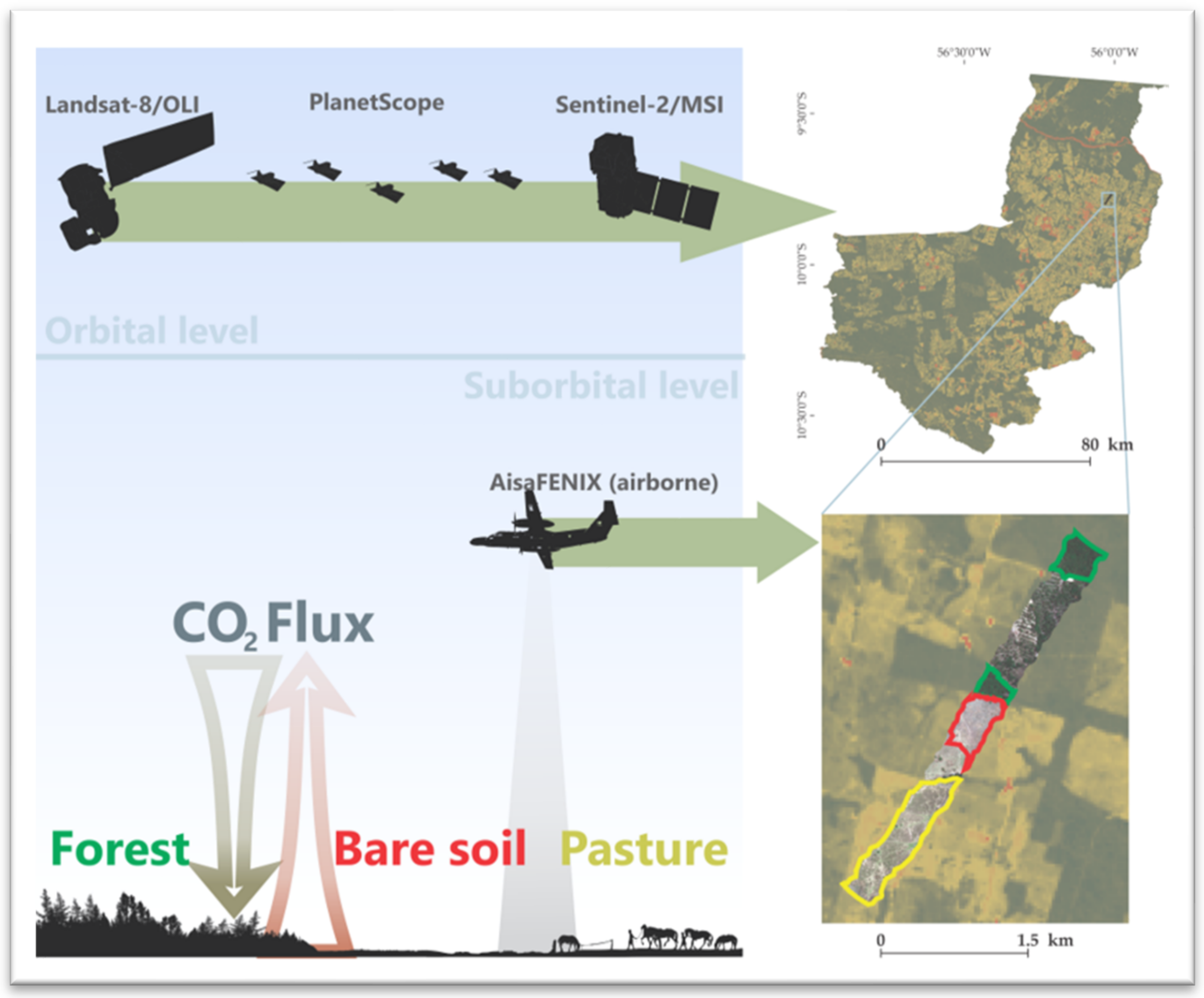
2.1. Study Site

This research was based on a Specim^® AisaFENIX image captured in the city of Alta Floresta (09°52′32″ S; 56°05′10″ W, altitude of 283 m), located in the northern part of the state of Mato Grosso, southern Brazilian Amazonia (Figure 1). With an average annual daily temperature of 26.4 °C, it is characterized by two well-defined climate seasons with high temperatures, the rainy and the dry season, classified as Aw according to Köppen–Geiger Climate Classification, and an average annual rainfall of 2281 mm.

The imaged area features primary tropical forest, pasture, and bare soil, which have different CO₂ emission and absorption patterns [42]. Four areas in the region of interest (ROI) were visually classified [43] as forest, bare soil, or pasture in order to sample ten random points for each land use type (i.e., into the polygon) in order to perform statistical analysis (Figure 2a). Aiming for a detailed quantification of different spectral models, we generated spectral profile plots based on a transect in the scene (Figure 2b).

2.2. Data Procurement and Image Pre-Processing

2.2.1. Hyperspectral Image

As mentioned above, the hyperspectral image (HSI) is based on Specim^® AisaFENIX, a push broom imaging hyperspectral spectrometer, which covers a spectral range from 380 to 2500 nm (visible, near infrared, and short-wave infrared) (Figure 3,

Table 1. Details of AisaFENIX system and data acquisition traits.

	VNIR 1	SWIR 2
Spectral range	380~970 nm	970~2500 nm
Spectral bands	344	275
Detector	Complementary metal-oxide-semiconductor (CMOS)	Mercury Cadmium Telluride (MCT) cooled detector
Spectral resolution	3.5 nm	12 nm
Field of View	32.3°
Focal aperture	F/2.4
Radiometric resolution	16 bits
Imaging speed	130 frames per second
Spatial resolution	0.65 m (at 600 m of altitude)

¹ VNIR: Visible and Near-Infrared; ² SWIR: Short-Wave Infrared.

). Data collection was conducted on 9 October 2017, onboard an aircraft. The radiometric and geometric corrections of the image were performed using CaliGeo Pro tool in ENVI, designed by Specim. This step included the use of (i) Look Up Table (.LUT) files, which have specific AisaFENIX parameters that need to be used during processing, and (ii) the dark reference files, which are the data captured in the same file as the image through its automatic activation (Auto Dark) and the radiometric calibration file (2 × 2) [32].

2.2.2. Orbital Data

Based on open access imagery, we have chosen OLI/Landsat-8, MSI/Sentinel-2, and PlanetScope data. The dates were chosen based on the nearest day of acquisition related to HSI data collection.

Data from Landsat-8 have medium spatial resolution varying from 15 to 100 m, and free-access data have abundant use in remote sensing. The OLI (Operational Land Imager) sensor has nine spectral (

Table 2. OLI/Landsat-8 spectral bands.

Band Name	Description	Spectral Range (nm)
B1	Coastal/Aerosol	433~453
B2	Blue	450~515
B3	Green	525~600
B4	Red	630~680
B5	Near Infrared	845~885
B6	SWIR 1	1560~1660
B7	SWIR 2	2100~2300
B8	Panchromatic	500~680
B9	Cirrus	1360~1390

) bands ranging from visible to short-wave infrared [44]. In this study, we used the required bands to calculate NDVI (band 4 for red and band 5 for near infrared) and the adapted PRI (band 2 for blue and band 3 for green), which have 30 m of spatial resolution.

In order to focus on free-access orbital data, the MSI sensor on board both Sentinel-2 mission satellites fits in this criterion. This imagery has medium spatial resolution ranging from 10 to 60 m, with 13 spectral bands (

Table 3. MSI/Sentinel-2 spectral bands.

Band Name	Description	Spectral Range (nm)
B01	Aerosols	421.7~463.7
B02	Blue	426.4~558.4
B03	Green	523.8~595.8
B04	Red	633.6~695.6
B05	Red edge 1	689.1~719.1
B06	Red edge 2	725.5~755.5
B07	Red edge 3	762.8~802.8
B08	Near infrared	726.8~938.8
B08a	Red edge 4	843.7~885.7
B09	Water vapor	925.1~965.1
B10	Cirrus	1342.5~1404.5
B11	SWIR 1	1522.7~1704.7
B12	SWIR 2	2027.4~2377.4

) from visible to short-wave infrared, similarly to the OLI/Landsat-8 system [45]. Here, the NDVI was based on bands 8 (Near infrared) and 4 (Red), while adapted PRI was calculated using bands 2 (Blue) and 3 (Green), with 10 m spatial resolution.

The third imagery assessed was PlanetScope. The PS2.SD instrument provides data on four spectral bands, between 464 and 888 nanometers with spatial resolution of 3 m (

Table 4. PlanetScope spectral bands.

Band Name	Spectral Range
Blue	464~517
Green	547~585
Red	650~682
NIR 1	846~888

¹ Near infrared.

). The whole spectral range is necessary to run the CO₂Flux model, where NDVI was based on red bands and NIR and PRI were based on blue and green bands.

The orbital data from OLI/Landsat-8 system were obtained on 6 October 2017. The study site was completely covered by one scene in this imagery. Regarding to Sentinel-2, it took two scenes to cover the entire study site, based on 14 October 2017. Last, PlanetScope image was acquired on 8 October 2017. The orbital data were acquired with radiometric calibration from Google Earth Engine and PlanetScope requisition, required to minimize scattering effect and other factors (

Table 5. Technical details of the scenes from different orbital platforms used in this study.

Imagery	Scene
OLI/Landsat-8	LANDSAT/LC08/C01/T1_RT_TOA/LC08_227067_20171006 1
MSI/Sentinel	20171014T140051_20171014T140051_T21LWK 1
	20171014T140051_20171014T140051_T21LXK 1
PlanetScope	Acquisition through PlanetScope requisition

¹ Acquisition through Google Earth Engine.

).

2.3. Data Processing

After acquisition (with atmospheric and shape correction), the AisaFENIX scene and the orbital data were resampled based on nearest neighbor algorithm in order to equalize spatial resolution among the different datasets. In this regard, AisaFENIX, PlanetScope, and MSI/Sentinel-2 data were lowered to 30 m of spatial resolution (Figure 4).

Following that, we calculated the indices on which the CO₂Flux emission model is based, namely, NDVI (Equation (1)), PRI (Equation (2)), scaled PRI (Equation (3)), and CO₂Flux (Equation (4)) itself. The selected bands to replace 531 nm and 570 nm on orbital datasets were blue and green bands respectively [16,33,34,35,36,37,38,39,40]. The AisaFENIX bands used in the VI calculation were those closer to the reference models, 62 for NIR and 42 for RED in NDVI equation, and bands 23 and 29 for 531 nm and 570 nm, respectively, in the PRI equation. Equation (4) shows the linear and angular (slope) coefficients presented on CO₂Flux modelling [24]. In this model, linear and angular coefficients are presented as NDVI and PRI vegetation models, and these coefficients should be adjusted according to environmental traits and are expressed in Equation (4) fitted to Amazonian patterns [40]:

$$\mathrm{NDVI}=\frac{{\rho }_{NIR}-{\rho }_{RED}}{{\rho }_{NIR}+{\rho }_{RED}},$$

(1)

$$\mathrm{PRI}=\frac{{\rho }_{531\mathrm{nm}}-{\rho }_{570\mathrm{nm}}}{{\rho }_{531\mathrm{nm}}+{\rho }_{570\mathrm{nm}}},$$

(2)

$$\mathrm{sPRI}=\frac{\mathrm{PRI}+1}{2},$$

(3)

$$\mathrm{C}{\mathrm{O}}_2\mathrm{F}\mathrm{l}\mathrm{u}\mathrm{x}=13.63-66.207\left(\mathrm{sPRI}\times \mathrm{NDVI}\right),$$

(4)

2.4. Statistical Approach

For each variable evaluated, we generated an analysis of variance (ANOVA). It was considered an entirely randomized design with 10 repetitions in a 4 × 3 factorial scheme (four sensors vs. three land use and land cover). Next, Tukey’s test was applied for multiple comparisons of means. In all cases, a 5% significance level was considered. The comparison among hyperspectral and multispectral profile transects was based on simple linear regression model and coefficient of determination (R²), with a p-value of 0.05.

3. Results

3.1. CO₂Flux

Initially, the spectral data from airborne and orbital systems were processed and underwent VI’s calculation. From this approach, the band math was carried out with NDVI (Figure 5), PRI (Figure 6), and mainly with CO₂Flux (Figure 7) in the ROI.

We generated the profile graphs (Figure 8) based on a north–south transect aligned to the scene, described in the OLI/Landsat-8 scene with RGB true color composition in Figure 2b. In the images, the lowest values on the horizontal axis from NDVI and PRI profiles refer to primary tropical forests (green), while increasing values in this axis refer to mixed forest and bare soil pixels (grey), turning to forest, then bare soil (red), and finally concerning pasture (yellow). In relation to the CO₂Flux, the opposite occurs. In Figure 8, it can be observed that the different curves for NDVI, PRI, and CO₂Flux are based on pixels collected in the transect within each image.

3.2. Statistical Approach

There were different significant interactions for the sensors and LULC types in all evaluated variables (Figure 9). In order to understand the Figure 9 results, there is no statistical difference when comparing sensors (lowercase) or LULC (uppercase) with same letter.

According to the spectral profile along the scene (Figure 2b), we compared the CO₂Flux values based on hyperspectral data to multispectral values with a simple linear regression model and the coefficient of determination (R²), presented in the scatterplot (Figure 10). A significance level of 0.05 was adopted, where these datasets tests showed correlation with lower than 0.05 significance probability (p-value). In this scatterplot, lower levels of CO₂Flux mostly represent tropical forest pixels, whereas light brown dots apply to bare soil and pasture pixels.

For NDVI (Figure 11), bare soil had no statistical difference between the sensors analyzed. However, the AisaFENIX sensor had the highest NDVI averages in comparison to multispectral sensors, mainly in forest and pasture, evidencing no statistical difference between MSI/Sentinel-2 and PLANET. In addition, it is observed that the forest presented the highest NDVI averages in relation to other LULC types, regardless of the sensor.

Regarding PRI or sPRI, we observed slight differences in inter-comparisons of the sensors, with higher mean absolute values on Landsat-8 results. Furthermore, among LULC types, tropical forest presented the highest mean values of PRI and sPRI on orbital datasets. OLI/Landsat-8 and PlanetScope data presented no statistical difference between pasture and bare soil for sPRI, as well as PRI on OLI/Landsat-8 data. Despite this, PRI values across the entire dataset were close to zero, regardless of LULC type and sensor. Turning to AisaFENIX results, PRI values were inversely related to orbital datasets, suggesting that further assessments using this sensor are required.

Concerning CO₂Flux, the AisaFENIX sensor showed the highest averages in relation to the others, independent of LULC type. CO₂Flux over bare soil (Figure 12) had no statistical difference among sensors. In addition, OLI/Landsat-8 had no statistical difference in tropical forest by comparing to MSI/Sentinel-2 (Figure 13). Regarding pasture, the OLI/Landsat-8 and PlanetScope results had no statistical difference (Figure 14). On the LULC prospect, bare soil presented the highest CO₂Flux values regardless of sensor, and an opposite scenario is observed with forest, which presented the lowest CO₂Flux values in comparison to other LULC types, regardless of the sensor.

4. Discussion

The atmospheric carbon uptake and emission phenomena assessment via remote sensing techniques can be based on either net ecosystem exchange (NEE) and CO₂Flux [24] estimations. In the first case, eddy flux tower collateral information and different micrometeorological computational tools and techniques are required [46]. On the other hand, CO₂Flux uses mainly remote sensing data.

Regarding the PRI, the substantial difference in this VI (and in its scaled version, sPRI) among sensors was evident, especially between different blue and green bands in the multispectral and hyperspectral bands. This difference is greater in open access imagery (Landsat-8 and Sentinel-2 systems) versus AisaFENIX, where both narrow PRI reference bands are in the green band for these datasets. It is noticeable that spectral mixing can occur in PRI results, since PlanetScope and AisaFENIX presented negative values for this VI, when OLI/Landsat-8 and MSI/Sentinel-2 presented values above zero in all LULC types.

The comparison between OLI and MSI on savanna areas and using resampling and similar atmospheric correction techniques reached root mean square difference of 0.0314, as showed in the study of [47], which could be assumed in our work, despite the fact that we analyze an evergreen tropical forest area. This similarity between results is greater when LULC classes which most resemble the savanna are observed, i.e., NDVI values in pasture and bare soil were statistically similar between PlanetScope and Sentinel-2/MSI comparison, and in turn, the CO₂Flux results from OLI/Landsat-8 and PlanetScope were statistically similar.

The lack of similarity among hyperspectral and multispectral sensors results from the analysis of variance approach suggests that spectral mixing can affect better outcomes, since NDVI and CO₂Flux had statistical similarity to PlanetScope to MSI/Sentinel-2 in the first VI and to OLI/Landsat-8 in the carbon model. We also highlight that environmental conditions related to drought may affect PRI performance [41,48], suggesting further assessment of CO₂Flux emission model considering temporal variations related to drought and rainfall seasonality is needed, since the performance of carbon sinks is related to canopy water content and vegetation structure [49].

The presence of NDVI on CO₂Flux rely on biomass measurement and its greenness [24], as NDVI performs best in leaf biomass estimation, where PlanetScope and Sentinel-2 data have been assessed as good predictors of aboveground biomass, which in turn evidences the greatest carbon pool in trees [50]. In remote sensing, the Gross Primary Production (GPP) is another metric for CO₂ balance, which expresses the uptake via photosynthesis and is less related to NDVI on LULC types with higher NDVI values [51]. In this scope, higher values of NDVI had lower correlation among datasets specially in forest areas, as in the PlanetScope versus Sentinel-2 comparison, which, in spatial variability, similar results were expected from phenological research work based on heterogeneous landscapes [52].

Atmospheric carbon dioxide uptake and emission assessed through the CO₂Flux model provides a metric related to land cover types, although it is limited in temporal variability. Considering land use change is more appropriate in the current scenario for the Amazonian rainforest, taking into account the rainfall seasonality and the climate variations that greatly affect the carbon uptake capacity of carbon sinks, is needed [53]. This suggests that the model is potentially functional when studying spatial-temporal dynamics in the Amazon biome.

The correlation among AisaFENIX and the different orbital datasets in this study based on linear regression expresses a greater reliance for CO₂Flux than discrete-sampling-based ANOVA. A spectral profile carries a larger data volume, which contributes to closely relating these results and could rely on analyzing different LULC types. Yet, the mean absolute error (MAE) and root mean squared error (RMSE) metrics similarly reported the difference among datasets seen on linear regression, whereas MSI/Sentinel-2 had the highest error value and lowest correlation. Based on this, further assessment within other land use types can improve remote sensing research devoted to carbon emission and dynamics.

In a broad observation of multispectral sensors results, the spectral mixing could affect CO₂Flux results, since PRI and the scaled version were lower in high spatial resolution sensors, i.e., PlanetScope and AisaFENIX. So far, the analysis of variance did not present the visual similarity between MSI/Sentinel-2 and AisaFENIX, which was expected since the variabilities in the scenes are similar in these datasets. On the other hand, the linear regression model and coefficient of determination suggest that the CO₂Flux model adapted to multispectral imagery reliably provides carbon flux estimation similar to hyperspectral sensor results. Despite the differences in the CO₂Flux from hyper- to multispectral sensors, NDVI achieved similarity in bare soil in all datasets, justifying further hyper-multispectral comparison studies, especially in the Amazon biome.

5. Conclusions

In this study, we developed an approach based on four different RS datasets in order to compare the CO₂Flux patterns within three land cover types in the southern part of Amazonia. We demonstrate that the CO₂Flux model can be based on open access orbital multispectral imagery when it comes to bare soil, for example. The results obtained in this study suggest that PlanetScope, MSI/Sentinel-2, OLI/Landsat-8, and AisaFENIX can be similarly scaled, that is, the data variabilities along a heterogeneous scene in evergreen tropical forest with different land uses are related. We highlight that the spatial-temporal dynamics of rainfall seasonality in relation to CO₂ emission and uptake should be assessed in future research. Our results provide a better understanding of how the aggregated use of different airborne and orbital datasets can provide reliable estimates of carbon emission and absorption within different terrestrial ecosystems in southern Amazonia.

References

1. Noon, M.L.; Goldstein, A.; Ledezma, J.C.; Roehrdanz, P.R.; Cook-Patton, S.C.; Spawn-Lee, S.A.; Wright, T.M.; Gonzalez-Roglich, M.; Hole, D.G.; Rockström, J.; et al. Mapping the irrecoverable carbon in Earth’s ecosystems. Nat. Sustain. 2021, 5, 37–46. [Google Scholar] [CrossRef]
2. Liu, J.; Huang, R.; Yu, K.; Zou, B. How lime-sand islands in the South China Sea have responded to global warming over the last 30 years: Evidence from satellite remote sensing images. Geomorphology 2020, 371, 107423. [Google Scholar] [CrossRef]
3. Wang, L.; Chen, L. Spatiotemporal dataset on Chinese population distribution and its driving factors from 1949 to 2013. Sci. Data 2016, 3, 160047. [Google Scholar] [CrossRef] [PubMed]
4. Gambo, J.; Ahmed Yusuf, Y.; Zulhaidi bin Mohd Shafri, H.; Salihu Lay, U.; Ahmed, A. A Three Decades Urban Growth Monitoring in Hadejia, Nigeria Using Remote Sensing and Geospatial Techniques. IOP Conf. Ser. Earth Environ. Sci. 2021, 620, 12012. [Google Scholar] [CrossRef]
5. Ma, A.; Chen, D.; Zhong, Y.; Zheng, Z.; Zhang, L. National-scale greenhouse mapping for high spatial resolution remote sensing imagery using a dense object dual-task deep learning framework: A case study of China. ISPRS J. Photogramm. Remote Sens. 2021, 181, 279–294. [Google Scholar] [CrossRef]
6. Zhang, Q.; Yuan, Q.; Zeng, C.; Li, X.; Wei, Y. Missing Data Reconstruction in Remote Sensing Image With a Unified Spatial–Temporal–Spectral Deep Convolutional Neural Network. IEEE Trans. Geosci. Remote Sens. 2018, 56, 4274–4288. [Google Scholar] [CrossRef] [Green Version]
7. Gerber, F.; de Jong, R.; Schaepman, M.E.; Schaepman-Strub, G.; Furrer, R. Predicting Missing Values in Spatio-Temporal Remote Sensing Data. IEEE Trans. Geosci. Remote Sens. 2018, 56, 2841–2853. [Google Scholar] [CrossRef] [Green Version]
8. Ponzoni, F.J.; Shimabukuro, Y.E. Sensoriamento Remoto no Estudo da Vegetação; Parêntese Editora: São José dos Campos, Brazil, 2009; ISBN 978-85-60507-02-3. [Google Scholar]
9. Ohyama, H.; Shiomi, K.; Kikuchi, N.; Morino, I.; Matsunaga, T. Quantifying CO2 emissions from a thermal power plant based on CO2 column measurements by portable Fourier transform spectrometers. Remote Sens. Environ. 2021, 267, 112714. [Google Scholar] [CrossRef]
10. Nassar, R.; Mastrogiacomo, J.-P.; Bateman-Hemphill, W.; McCracken, C.; MacDonald, C.G.; Hill, T.; O’Dell, C.W.; Kiel, M.; Crisp, D. Advances in quantifying power plant CO2 emissions with OCO-2. Remote Sens. Environ. 2021, 264, 112579. [Google Scholar] [CrossRef]
11. Lei, R.; Feng, S.; Danjou, A.; Broquet, G.; Wu, D.; Lin, J.C.; O’Dell, C.W.; Lauvaux, T. Fossil fuel CO2 emissions over metropolitan areas from space: A multi-model analysis of OCO-2 data over Lahore, Pakistan. Remote Sens. Environ. 2021, 264, 112625. [Google Scholar] [CrossRef]
12. Guo, M.; Li, J.; Xu, J.; Wang, X.; He, H.; Wu, L. CO2 emissions from the 2010 Russian wildfires using GOSAT data. Environ. Pollut. 2017, 226, 60–68. [Google Scholar] [CrossRef] [PubMed]
13. Du, S.; Liu, L.; Liu, X.; Zhang, X.; Zhang, X.; Bi, Y.; Zhang, L. Retrieval of global terrestrial solar-induced chlorophyll fluorescence from TanSat satellite. Sci. Bull. 2018, 63, 1502–1512. [Google Scholar] [CrossRef] [Green Version]
14. Li, S.; Gao, M.; Li, Z.-L.; Duan, S.; Leng, P. Uncertainty analysis of SVD-based spaceborne far–red sun-induced chlorophyll fluorescence retrieval using TanSat satellite data. Int. J. Appl. Earth Obs. Geoinf. 2021, 103, 102517. [Google Scholar] [CrossRef]
15. Fernandez, H.M.; Granja-Martins, F.M.; Pedras, C.M.G.; Fernandes, P.; Isidoro, J.M.G.P. An Assessment of Forest Fires and CO2 Gross Primary Production from 1991 to 2019 in Mação (Portugal). Sustainability 2021, 13, 5816. [Google Scholar] [CrossRef]
16. Souza, A.P.D.; Teodoro, P.E.; Teodoro, L.P.R.; Taveira, A.C.; de Oliveira-Júnior, J.F.; Della-Silva, J.L.; Baio, F.H.R.; Lima, M.; da Silva Junior, C.A. Application of remote sensing in environmental impact assessment: A case study of dam rupture in Brumadinho, Minas Gerais, Brazil. Environ. Monit. Assess. 2021, 193, 606. [Google Scholar] [CrossRef] [PubMed]
17. Chen, Y.; Guerschman, J.P.; Cheng, Z.; Guo, L. Remote sensing for vegetation monitoring in carbon capture storage regions: A review. Appl. Energy 2019, 240, 312–326. [Google Scholar] [CrossRef]
18. Lees, K.J.; Quaife, T.; Artz, R.R.E.; Khomik, M.; Clark, J.M. Potential for using remote sensing to estimate carbon fluxes across northern peatlands—A review. Sci. Total Environ. 2018, 615, 857–874. [Google Scholar] [CrossRef]
19. Xiao, J.; Chevallier, F.; Gomez, C.; Guanter, L.; Hicke, J.A.; Huete, A.R.; Ichii, K.; Ni, W.; Pang, Y.; Rahman, A.F.; et al. Remote sensing of the terrestrial carbon cycle: A review of advances over 50 years. Remote Sens. Environ. 2019, 233, 111383. [Google Scholar] [CrossRef]
20. Angelopoulou, T.; Tziolas, N.; Balafoutis, A.; Zalidis, G.; Bochtis, D. Remote Sensing Techniques for Soil Organic Carbon Estimation: A Review. Remote Sens. 2019, 11, 676. [Google Scholar] [CrossRef] [Green Version]
21. McClelland, M.P.; van Aardt, J.; Hale, D. Manned aircraft versus small unmanned aerial system—forestry remote sensing comparison utilizing lidar and structure-from-motion for forest carbon modeling and disturbance detection. J. Appl. Remote Sens. 2019, 14, 022202. [Google Scholar] [CrossRef]
22. Fernández-Guisuraga, J.M.; Suárez-Seoane, S.; Fernandes, P.M.; Fernández-García, V.; Fernández-Manso, A.; Quintano, C.; Calvo, L. Pre-fire aboveground biomass, estimated from LiDAR, spectral and field inventory data, as a major driver of burn severity in maritime pine (Pinus pinaster) ecosystems. For. Ecosyst. 2022, 9, 100022. [Google Scholar] [CrossRef]
23. De Almeida, C.T.; Galvão, L.S.; de Oliveira Cruz e Aragão, L.E.; Ometto, J.P.H.B.; Jacon, A.D.; de SouzaPereira, F.R.; Sato, L.Y.; Lopes, A.P.; Lima de Alencastro Graça, P.M.; de Jesus Silva, C.V.; et al. Combining LiDAR and hyperspectral data for aboveground biomass modeling in the Brazilian Amazon using different regression algorithms. Remote Sens. Environ. 2019, 232, 111323. [Google Scholar] [CrossRef]
24. Rahman, A.F.; Gamon, J.A.; Fuentes, D.A.; Roberts, D.A.; Prentiss, D. Modeling spatially distributed ecosystem flux of boreal forest using hyperspectral indices from AVIRIS imagery. J. Geophys. Res. Atmos. 2001, 106, 33579–33591. [Google Scholar] [CrossRef]
25. Garbulsky, M.F.; Peñuelas, J.; Gamon, J.; Inoue, Y.; Filella, I. The photochemical reflectance index (PRI) and the remote sensing of leaf, canopy and ecosystem radiation use efficiencies: A review and meta-analysis. Remote Sens. Environ. 2011, 115, 281–297. [Google Scholar] [CrossRef]
26. Peñuelas, J.; Inoue, Y. Reflectance assessment of canopy CO2 uptake. Int. J. Remote Sens. 2000, 21, 3353–3356. [Google Scholar] [CrossRef]
27. Migliavacca, M.; Galvagno, M.; Cremonese, E.; Rossini, M.; Meroni, M.; Sonnentag, O.; Cogliati, S.; Manca, G.; Diotri, F.; Busetto, L.; et al. Using digital repeat photography and eddy covariance data to model grassland phenology and photosynthetic CO2 uptake. Agric. For. Meteorol. 2011, 151, 1325–1337. [Google Scholar] [CrossRef]
28. Rouse, J.W., Jr.; Haas, R.H.; Schell, J.A.; Deering, D.W. Monitoring Vegetation Systems in the Great Plains with ERTS. In Proceedings of the ERTS-1 Symposium, Washington, DC, USA, 10–14 December 1973; Volume 351, p. 309. [Google Scholar]
29. Gamon, J.; Serrano, L.; Surfus, J.S. The Photochemical Reflectance Index: An Optical Indicator of Photosynthetic Radiation Use Efficiency across Species, Functional Types, and Nutrient Levels. Oecologia 1997, 112, 492–501. [Google Scholar] [CrossRef]
30. Gamon, J.A.; Peñuelas, J.; Field, C.B. A narrow-waveband spectral index that tracks diurnal changes in photosynthetic efficiency. Remote Sens. Environ. 1992, 41, 35–44. [Google Scholar] [CrossRef]
31. Drolet, G.G.; Huemmrich, K.F.; Hall, F.G.; Middleton, E.M.; Black, T.A.; Barr, A.G.; Margolis, H.A. A MODIS-derived photochemical reflectance index to detect inter-annual variations in the photosynthetic light-use efficiency of a boreal deciduous forest. Remote Sens. Environ. 2005, 98, 212–224. [Google Scholar] [CrossRef]
32. SPECIM AisaFENIX—Specim. Available online: https://www.specim.fi/products/aisafenix/ (accessed on 29 March 2021).
33. Barnes, M.L.; Farella, M.M.; Scott, R.L.; Moore, D.J.P.; Ponce-Campos, G.E.; Biederman, J.A.; MacBean, N.; Litvak, M.E.; Breshears, D.D. Improved dryland carbon flux predictions with explicit consideration of water-carbon coupling. Commun. Earth Environ. 2021, 2, 248. [Google Scholar] [CrossRef]
34. Da Silva Junior, C.A.; de MedeirosCosta, G.; Saragosa Rossi, F.; Evangelista doVale, J.C.; Bruto de Lima, R.B.; Lima, M.; de Oliveira-Junior, J.F.; Teodoro, P.E.; Santos, R.C. Remote sensing for updating the boundaries between the brazilian Cerrado-Amazonia biomes. Environ. Sci. Policy 2019, 101, 383–392. [Google Scholar] [CrossRef]
35. Polonio, V.D. Índices de Vegetação na Mensuração do Estoque de Carbono em Áreas com Cana-de-Açúcar; UNESP: São Paulo, Brazil, 2015. [Google Scholar]
36. Do Nascimento Lopes, E.R.; de Sousa, J.A.P.; de Souza, J.C.; Filho, J.L.A.; Lourenço, R.W. Spatial dynamics of Atlantic Forest fragments in a river basin. Floresta 2019, 50, 1053. [Google Scholar] [CrossRef] [Green Version]
37. Fernandez, H.M.; Gomes, C.P.; Granja-Martins, F.M. Monitorização por satélite da desflorestação da floresta do Maiombe em Cabinda, Angola nos últimos 33 anos. Rev. GEAMA—Ciências Ambient. Biotecnol. 2020, 6, 81–91. [Google Scholar]
38. Correia Filho, W.L.F.; de Barros Santiago, D.; de Oliveira-Júnior, J.F.; da Silva Junior, C.A.; da Silva Oliveira, S.R.; da Silva, E.B.; Teodoro, P.E. Analysis of environmental degradation in Maceió-Alagoas, Brazil via orbital sensors: A proposal for landscape intervention based on urban afforestation. Remote Sens. Appl. Soc. Environ. 2021, 24, 100621. [Google Scholar] [CrossRef]
39. Rossi, F.S.; de Araújo Santos, G.A.; de Souza Maria, L.; Lourençoni, T.; Pelissari, T.D.; Della-Silva, J.L.; Júnior, J.W.O.; de Avila e Silva, A.; Lima, M.; Teodoro, P.E.; et al. Carbon dioxide spatial variability and dynamics for contrasting land uses in central Brazil agricultural frontier from remote sensing data. J. South Am. Earth Sci. 2022, 116, 103809. [Google Scholar] [CrossRef]
40. Dos Santos, C.V.B. Modelagem Espectral para Determinação de Fluxo de CO2 em Áreas de Caatinga Preservada e em Regeneração Cloves. Master’s Thesis, Universidade Estadual de Feira de Santana, Novo Horizonte, Brazil, 2017. [Google Scholar]
41. Inoue, Y.; Peñuelas, J.; Miyata, A.; Mano, M. Normalized difference spectral indices for estimating photosynthetic efficiency and capacity at a canopy scale derived from hyperspectral and CO2 flux measurements in rice. Remote Sens. Environ. 2008, 112, 156–172. [Google Scholar] [CrossRef]
42. Ostle, N.J.; Levy, P.E.; Evans, C.D.; Smith, P. UK land use and soil carbon sequestration. Land Use Policy 2009, 26, S274–S283. [Google Scholar] [CrossRef]
43. Hölbling, D.; Eisank, C.; Albrecht, F.; Vecchiotti, F.; Friedl, B.; Weinke, E.; Kociu, A. Comparing Manual and Semi-Automated Landslide Mapping Based on Optical Satellite Images from Different Sensors. Geosciences 2017, 7, 37. [Google Scholar] [CrossRef] [Green Version]
44. Landsat 8. U.S. Geological Survey. Available online: https://www.usgs.gov/landsat-missions/landsat-8 (accessed on 3 January 2022).
45. MSI Instrument—Sentinel-2 MSI Technical Guide—Sentinel Online—Sentinel. Available online: https://sentinels.copernicus.eu/web/sentinel/technical-guides/sentinel-2-msi/msi-instrument (accessed on 3 January 2022).
46. Zhang, C.; Brodylo, D.; Sirianni, M.J.; Li, T.; Comas, X.; Douglas, T.A.; Starr, G. Mapping CO2 fluxes of cypress swamp and marshes in the Greater Everglades using eddy covariance measurements and Landsat data. Remote Sens. Environ. 2021, 262, 112523. [Google Scholar] [CrossRef]
47. Zhang, H.K.; Roy, D.P.; Yan, L.; Li, Z.; Huang, H.; Vermote, E.; Skakun, S.; Roger, J.-C. Characterization of Sentinel-2A and Landsat-8 top of atmosphere, surface, and nadir BRDF adjusted reflectance and NDVI differences. Remote Sens. Environ. 2018, 215, 482–494. [Google Scholar] [CrossRef]
48. Hwang, T.; Gholizadeh, H.; Sims, D.A.; Novick, K.A.; Brzostek, E.R.; Phillips, R.P.; Roman, D.T.; Robeson, S.M.; Rahman, A.F. Capturing species-level drought responses in a temperate deciduous forest using ratios of photochemical reflectance indices between sunlit and shaded canopies. Remote Sens. Environ. 2017, 199, 350–359. [Google Scholar] [CrossRef]
49. Asner, G.P.; Brodrick, P.G.; Anderson, C.B.; Vaughn, N.; Knapp, D.E.; Martin, R.E. Progressive forest canopy water loss during the 2012–2015 California drought. Proc. Natl. Acad. Sci. USA 2016, 113, E249–E255. [Google Scholar] [CrossRef] [PubMed] [Green Version]
50. Baloloy, A.B.; Blanco, A.C.; Candido, C.G.; Argamosa, R.J.L.; Dumalag, J.B.L.C.; Dimapilis, L.L.C.; Paringit, E.C. Estimation of mangrove forest aboveground biomass using multispectral bands, vegetation indices and biophysical variables derived from optical satellite imageries: RapidEye, PlanetScope and Sentinel-2. In Proceedings of the ISPRS Annals of the Photogrammetry, Remote Sensing and Spatial Information Sciences, Beijing, China, 7–10 May 2018. [Google Scholar]
51. Menefee, D.; Rajan, N.; Cui, S.; Bagavathiannan, M.; Schnell, R.; West, J. Carbon exchange of a dryland cotton field and its relationship with PlanetScope remote sensing data. Agric. For. Meteorol. 2020, 294, 108130. [Google Scholar] [CrossRef]
52. Cheng, Y.; Vrieling, A.; Fava, F.; Meroni, M.; Marshall, M.; Gachoki, S. Phenology of short vegetation cycles in a Kenyan rangeland from PlanetScope and Sentinel-2. Remote Sens. Environ. 2020, 248, 112004. [Google Scholar] [CrossRef]
53. Asner, G.P.; Nepstad, D.; Cardinot, G.; Ray, D. Drought stress and carbon uptake in an Amazon forest measured with spaceborne imaging spectroscopy. Proc. Natl. Acad. Sci. USA 2004, 101, 6039–6044. [Google Scholar] [CrossRef] [Green Version]
Figure 1. Description of the imaged area in Alta Floresta, Mato Grosso, Brazil.
Sustainability 14 05458 g001
Figure 2. (a) Regions of interest, classified as forest (green), bare soil (red), and pasture (yellow) areas; (b) spectral profile transect over the OLI/Landsat-8 scene.
Sustainability 14 05458 g002
Figure 3. Equipment used in the airborne imaging of the study area.
Sustainability 14 05458 g003
Figure 4. (a) AisaFENIX scene to resampled (b) scene (RGB composition on bands 42, 26, and 12). Scene detail from original (c) and resampled (d) image.
Sustainability 14 05458 g004
Figure 5. Normalized Difference Vegetation Index (NDVI) results for OLI/Landsat-8 (a), MSI/Sentinel-2 (b), PlanetScope (c), and AisaFENIX (d) imagery.
Sustainability 14 05458 g005
Figure 6. Photochemical Reflectance Index (PRI) results for OLI/Landsat-8 (a), MSI/Sentinel-2 (b), PlanetScope (c), and AisaFENIX (d) imagery.
Sustainability 14 05458 g006
Figure 7. CO2Flux emission (μmol m−2 s−1) results for OLI/Landsat-8 (a), MSI/Sentinel-2 (b), PlanetScope (c), and AisaFENIX (d) imagery.
Sustainability 14 05458 g007
Figure 8. NDVI, PRI, and CO2Flux spectral profiles based on the transect described in Figure 2b t. Horizontal axis refers to the spatial variation over the transect line (kilometers), while vertical axis represents the index value for NDVI, PRI, and μmol m−2 s1 for CO2Flux.
Sustainability 14 05458 g008
Figure 9. Significant interaction among sensors versus LULC for the vegetation indices NDVI, PRI, sPRI, and CO2Flux. Uppercase letters express statistical similarity or difference on by comparing LULC for the same sensor, and lowercase letters express statistical similarity or difference on the same LULC for different sensors.
Sustainability 14 05458 g009
Figure 10. Linear regressions and trend lines based on AisaFENIX versus (a) OLI/Landsat-8, (b) MSI/Sentinel-2, and (c) PlanetScope results of CO2Flux.
Sustainability 14 05458 g010
Figure 11. NDVI on bare soil area (blue polygon) based on OLI/Landsat-8 (a), MSI/Sentinel-2 (b), PlanetScope (c), and AisaFENIX (d) images.
Sustainability 14 05458 g011
Figure 12. CO2Flux on bare soil area (blue polygon) based on Landsat-8 (a), Sentinel-2 (b), PLANET (c), and AisaFENIX (d) images.
Sustainability 14 05458 g012
Figure 13. CO2Flux on tropical forest areas (blue polygons) based on OLI/Landsat-8 (a), Sentinel-2 (b), PLANET (c), and AisaFENIX (d) images.
Sustainability 14 05458 g013
Figure 14. CO2Flux on pasture area (blue polygon) based on OLI/Landsat-8 (a), Sentinel-2 (b), PLANET (c), and AisaFENIX (d) images.
Sustainability 14 05458 g014