Shaking Table Test and Numerical Simulation Study on Tunnel-Soil-Bridge Pile Structure Interaction System

Abstract

In this study, based on the actual project in Dalian, the dynamic interaction of the double tunnel sand bridge pile system (SSSI) under earthquake action is studied by shaking table test, and the dynamic response laws of the structure and site are obtained, which are compared with ABAQUS numerical simulation. The Kelvin constitutive model subprogram is introduced into the numerical model, and the equivalent linear method is used to deal with the nonlinear problems of sand in the calculation process. The experimental results are compared with the results obtained using the numerical model to verify the reliability of the numerical simulation. Based on this, eight working conditions are designed, and the interaction law between the structures in the system is investigated through a comparative analysis. The results showed that the tunnel amplifies the dynamic responses of the bridge pile, adjacent tunnel, and far field, while the bridge pile attenuates the dynamic responses of the side tunnel and far field; the presence of both the tunnel and bridge pile increases the internal force of the adjacent structure, and the peak internal force often occurs near the intersection of the structure or at the pile–soil interface.

1. Introduction

In recent years, the world has entered a golden period of underground space development and utilization. With the development of construction technology, a significant breakthrough has been made in the construction of underground structures in terms of their size and scale. Given the limited urban underground space resources, there has been an increasing number of close crossing projects between underground and above-ground structures.

The existence of underground structures destroys the integrity of the soil, and the multiple reflections and refractions of seismic waves by underground structures affect the dynamic response characteristics of the soil in the site and thus the seismic response of the neighboring above-ground structures. In addition, the fluctuation field and additional stress field due to the inertia of the above-ground structures cause disturbances to the site soil and thus affect the seismic response of underground structures. For example, many underground projects and adjacent above-ground structures were damaged during the Hanshin earthquake in Japan [1], the Jiji earthquake in Taiwan [2] and the Wenchuan earthquake, the above-ground structure–soil–underground structure interaction has attracted research attention. Chen et al. [3] and Wang et al. [4] believed that the existence of underground structures cannot be ignored for the influence of surface structures. Lou et al. [5] emphasized the importance of surface structure–soil–underground structure interaction. The surface structure–soil–subsurface structure interaction should be considered in the structural design. Therefore, to ensure the overall seismic disaster prevention capability of cities, it is necessary to consider the seismic performance of both underground and adjacent above-ground structures, to study the seismic response law of the above-ground structure–soil–underground structure system as a whole, and to establish a simple, practical, reasonable, and feasible seismic analysis method.

With the development of computer technology, numerical methods for subsurface structures have emerged, including the substructure method, finite element method, and hybrid method [6]. Since numerical simulation methods are more economical and can be verified using shaking table test results to investigate the seismic response law of underground structures, they have become a favored research method. Many domestic and foreign scholars have studied the effects of different factors on the seismic response of the complex system of above-ground structure–soil–underground structures.

Abate et al. [7] systematically studied the seismic response of a tunnel–soil–superstruc-ture interaction system in the context of an actual Italian project. The results showed that the presence of the tunnel played a certain function of seismic isolation. Dashti et al. [8] designed and implemented a series of centrifuge shaking table tests on an aboveground structure–soil–subsurface structure interaction system, and analyzed the rationality of the test scheme based on the test results. Pitilakis et al. [9] investigated the effect of surface structures on the seismic response of adjacent tunnels using a 2D numerical approach. The presence of adjacent surface structures was found to increase the seismic response of shallow–buried tunnels. Chen et al. [10] conducted a 2D finite element simulation analysis of a multistory basement-pile-twin-tower high-rise building and found that the effect of soil–structure interaction on the seismic response of the high-rise building is related to the site conditions and input ground shaking; the softer the site, the more significant the interaction effect. Chen et al. [11] and He et al. [12] studied the two-dimensional seismic response law of underground structure-soil-surface structure against the background of actual engineering. The study found that the existence of underground structure would increase the seismic response of a certain range of soil surface and surface structure. Lia et al. [13] performed 3D nonlinear finite element simulation of a subway station considering the effects of vertical ground shaking and the depth of the structural cover. The results showed that the consideration of vertical seismic motion increases the seismic response of the structure; the degree of this effect depends largely on the characteristics of the vertical seismic excitation. Miao et al. [14] studied the dynamic interaction of a system comprising multiple above-ground buildings, soils, and subway stations under the action of ground motions through an automatic modeling system. The numerical calculation results showed that several key factors, such as the number of buildings and the depth of burial, significantly amplify or attenuate the seismic response of underground structures.

With urbanization, an increasing number of taller and smaller urban buildings are urban building clusters. The shaking of building complexes during earthquakes will reflect a part of the ground shaking energy into the foundation soil, thus changing the dynamic response of the soil; this is the structure–soil–structure interaction (SSSI) that is currently receiving much attention. However, most current research has focused on 2D or frequency–domain analyses; studies on 3D models considering the nonlinearity of the soil are lacking. Three-dimensional models can more accurately reflect the characteristics of complex structural systems with a complex spatial distribution, and the soil nonlinearity has a non-negligible impact on the seismic resistance of such systems. Therefore, it is necessary to conduct further research on the SSSI system considering 3D model of the soil nonlinearity.

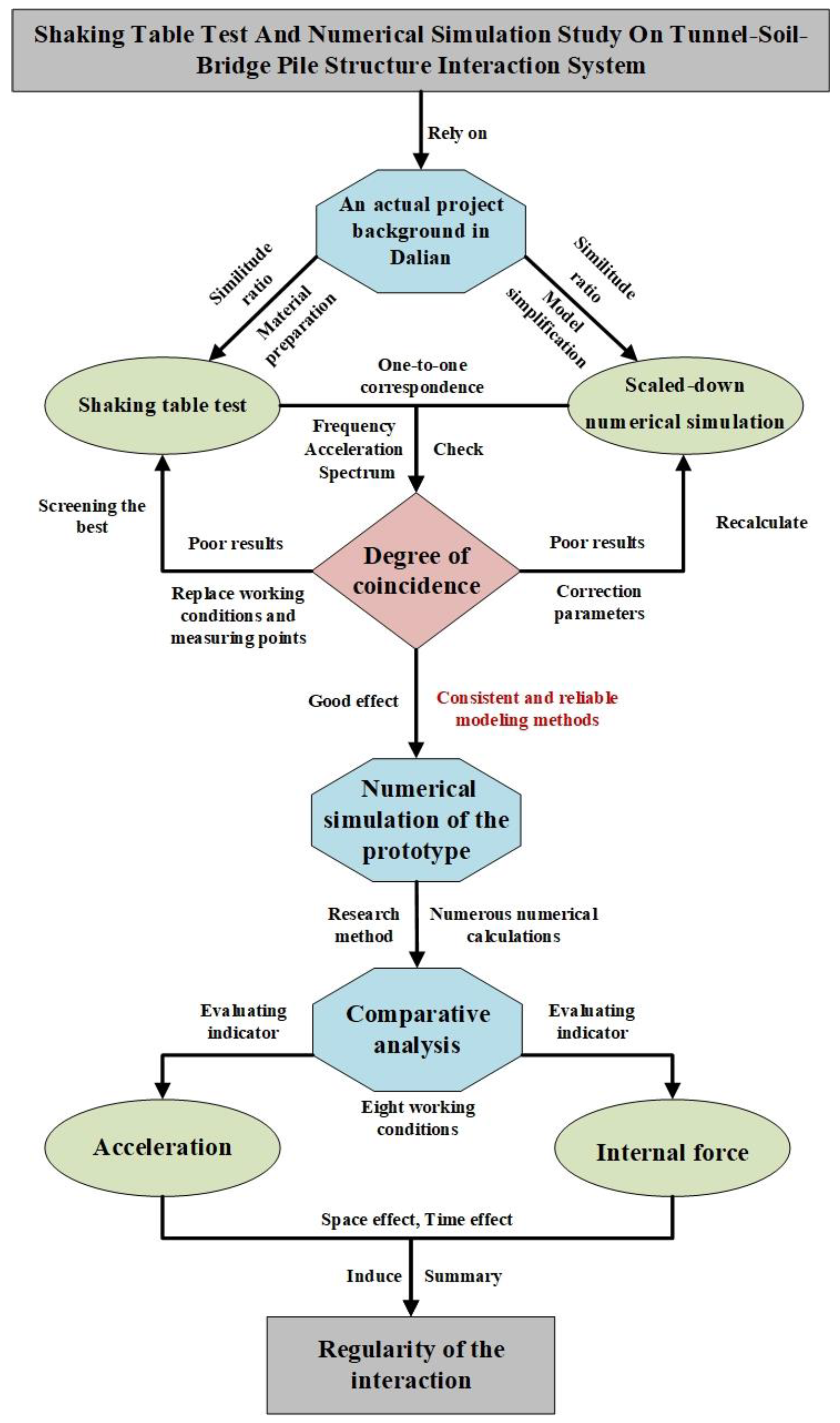
This study adopts shaking table experiments and numerical simulation research methods in the context of an actual project. The reliability of the numerical modeling is first verified through experiments, and the verified numerical models are then compared and analyzed to reveal the variation laws of the peak acceleration and internal force of the tunnel and bridge pile under different working conditions.

A preliminary and systematic study is conducted on the interaction law of the tunnel–soil–bridge pile structure system under the action of earthquakes. It provides a reference and guidance for studying the regularity of the seismic damage and can aid the structural design of bridge pile structures and underground tunnel structures. As shown in Figure 1, is the flow chart of the article.

2. Shaking Table Test

Taking the standard diameter shield section of the interval between Dalian Railway Station Station–Soyuwan South Station in China at a mileage of YK9+642.835 as the background, the planar relationship between the tunnel and the express rail line 3 and the cross-sectional relationship between the tunnel and the express rail line 3 are shown in Figure 2. From Figure 2, it can be found that there is a real working condition of double tunnel crossing bridge piles. When an earthquake occurs, there will be complex dynamic interaction between the tunnel and bridge piles. Therefore, it is necessary to conduct experimental and numerical simulation analysis on the tunnel soil tunnel interaction system at this location. A series of shaking table tests were designed on this basis.

2.1. Shaking Table and Model Container

The Shaking table tests were conducted on an earth-quake simulation shaker at Liaoning University of Engineering and Technology. The shaking table has a platform size of 3 m × 3 m, a maximum payload of 10 t, and an operating frequency ranging from 0 Hz to 50 Hz. The rigid box has the advantages of easy fabrication and easy numerical simulation over the flexible shear box. Ma et al. [15] verified the feasibility of a soft-lined rigid model box. The rigid box was welded and fixed to the steel platform of the shaker. The model box size is 2 m × 2 m × 1.5 m, surrounded by a 200 mm-thick polystyrene foam board, fixed on the side wall to reduce the boundary effect, as shown in Figure 3. The soil size is 1.6 m × 1.6 m × 1.3 m considering the polystyrene foam board and the bridge pile structure.

2.2. Design of Similarity Ratio

For the choice of the model material, particulate concrete is generally used to simulate the elastic-plastic seismic response of structures. However, Plexiglas was chosen in the test to consider the elastic seismic response law of the system. Plexiglass has the advantages of good homogeneity, high strength, and low modulus of elasticity [16]. The sandy soil [17,18,19] was chosen as the model soil, with a density of 1614 kg/m³ and a shear wave velocity of 55 m/s². The density of the Plexiglas is 1180 kg/m³, and the modulus of elasticity is 3 GPa. For prototype structure, the elastic modulus of bridge pile (C30), mine tunnel (C45) and shield tunnel (C50) are 30 Gpa, 33.5 Gpa, 34.5 Gpa respectively, and the density is 2500 kg/m³. The corresponding similarity ratio of the density is 0.442, and the similarity ratios of the modulus of elasticity are 0.1 (bridge pile), 0.09 (mine tunnel), and 0.087 (shield tunnel). Considering the size of the prototype structure and the size limitation of the model box in the shaking table test, the geometric similarity ratio of the test is selected as 1/30. After the three basic similarity ratios of the test model and the prototype structure, namely geometric similarity ratio, density similarity ratio, and elastic modulus similarity ratio, are determined, the similarity ratios between other physical quantities can be derived using Buckingham’s law [20].

Table 1. Similarity ratios of the model structure and tunnel.

Physical Quantities	Symbol	Similarity Ratio
Length	$l_r$	0.0333
Elastic modulus	$E_r$	0.1/0.09/0.087
Equivalent density	${\rho }_r$	0.472
Stress	${\sigma }_r=E_r$	0.1/0.09/0.087
Time	$t_r=l_r^{0.5}$	0.183
Displacement	$r_r=l_r$	0.0333
Velocity	$v_r=l_r^{0.5}$	0.183
Acceleration	$a_r=1$	1
Frequency	${\omega }_r=l_r^{-0.5}$	5.477

When the similarity ratio is different, it corresponds to bridge pile/mine tunnel/shield tunnel in turn.

presents the similarity ratios between the bridge piles and tunnels.

2.3. Model Structure and Instrumentation

Based on the actual engineering background and combined with the similarity ratio, a plexiglass model of the bridge pile and the tunnel was made and counterweighted. Considering the limited size of the model box and the boundary effect, the length of the tunnel was 0.7 m. The masses were added to the model surface structure and tunnel to meet the density similarity ratio, match the performance of the shaking table, and keep the acceleration and frequency similarity ratios within a reasonable range. The artificial mass is calculated according to the following formula [21]:

$$m_a=E_r{l}_r^2{m}_p-m_m$$

(1)

where $m_a$ is the artificial mass, $E_r$ is the elastic modulus similarity ratio, $l_r$ is geometric similarity ratio, $m_p$ is the total mass of the prototype structure, $m_m$ is the model structure quality. After the calculation, masses of 120, 60, and 30 kg were added to the bridge piles and the left and right tunnel structures, respectively. The acceleration was recorded using a Donghua power collector DH5922D, and the strain and earth pressure were recorded using a Donghua strain collector DH3817K. Figure 4 shows the model, counterweight, and collector.

2.4. Test Items and Measurement Point Arrangement

The test was divided into two stages: free field (FF) and dual tunnel–soil–bridge piles (DTSP). Each stage includes the same seismic wave input, as shown in Figure 5. The time interval was determined by the original time interval of 0.02 s and a time similarity ratio of 0.183. Moreover, considering the ability of the shaker control system, a time interval of 0.00125 s was selected in the experiment.

In the experiment, the acceleration responses of the tunnel, the bridge piles, and the surrounding soil, the strain of tunnel lining, and contact pressure between the model structure and the surrounding soil were measured. The sensors used in the shaking table test included accelerometers, strain gauges, and soil pressure gauges. The terms describing the sensor are as follows: A means the acceleration, S means the strain gauge, and P means the earth pressure gauge. Due to the different test objectives, the sensor arrangement of each test stage is also different. Figure 6 shows the sensor arrangement.

The measuring points are mainly distributed on the side of the tunnel close to the bridge pile, pile body, and soil surface according to the law. The main focus is on the measurement points A19, A02, A07, A12, A11, and A06 at the upper and lower ends of the tunnel and bridge piles for comparison with the subsequent numerical simulation results. In addition, after testing, the tunnel structure was excavated, and it was found that there was no damage to the tunnel structure. At the same time, it was found that the tunnel monitoring strain was excessively small. Therefore, only the acceleration response of the structure is given in the following.

The transfer function method was used to measure the intrinsic frequency of the system during the experiments. In the transfer function method, the frequency response function (FRF) is defined as the ratio of the recorded acceleration time course to the input time course. Figure 7a,b shows the transfer functions of A14 in the free field and A14 in the double tunnel–soil–pile in WN0.1g, respectively.

3. Numerical Simulation

3.1. Scaled-Down Numerical Simulation

A numerical model of the shaking table test was established using the finite element analysis software ABAQUS, as shown in Figure 8, the total number of elements and nodes of the numerical model are 54,155 and 65,156 respectively. The first-order intrinsic frequencies under the two working conditions were calculated using the material parameters given by the shaking table test and compared with the experimental results, as presented in

Table 2. Comparison between numerical and experimental results of the natural frequency.

Working Condition	Numerical Result	Experimental Result
DTSP	13.679 Hz	13.419 Hz
FF	16.228 Hz	15.350 Hz

. El-Centro wave, Taft wave, and Chichi wave ground vibrations were inputted to the free-field and tunnel–soil–bridge pile systems with reference to the shaking table test.

To verify the reliability of the numerical model, the acceleration peaks obtained from the numerical simulation were compared with those recorded from the shaker test, as presented in

Table 3. Comparison of numerical and test results in the peak response accelerations (unit: m/s²).

Points	Numerical Results	Test Results
A19	4.551	4.802 (5.32%)
A02	2.554	2.029 (25.87%)
A07	2.527	1.921 (31.56%)
A12	2.345	1.911 (22.71%)
A11	2.011	1.832 (9.77%)
A06	1.930	1.734 (11.30%)

The input wave is EI, the acceleration amplitudes are 1.3 m/s²; The data in parentheses is the difference ratio.

, and the differences were found to be within 30%. Figure 9a,b shows the acceleration–time course and Fourier spectra of the A02 and A19 sensors under DTSP, respectively. The Fourier amplitude spectrum results shown in Figure 8 are normalized to a value equal to the data divided by its maximum value, as shown in Figure 10a,b. It can be seen from the Fourier spectrum that there are some differences in the frequency components between the test results and the simulation results, which may be due to the simplification of the soil model and the shaking table. The former may play a filtering role, while the latter may produce some high-frequency interference noise mixed with ground motion [14]. In general, the first natural frequency of the seismic wave at the test and simulated monitoring points is relatively close. In combination with the peak value and waveform of the acceleration time history curve of the two, the results of numerical simulation are relatively reliable.

In this section, based on a series of shaking table tests on the seismic response of the system composed of tunnels, soil and bridge piles, the corresponding scale numerical simulation is carried out. The validity of the numerical modeling method is verified by comparing the experimental results with the scaled numerical results in terms of system fundamental frequency, acceleration curve and Fourier spectrum curve. In the following prototype numerical modeling process, a consistent modeling method is adopted, in which the similarity relationship is satisfied in the modeling process of tunnel and bridge pile structures, and the soil mass is large enough considering the influence of one-way excitation and boundary conditions. Details of the modeling process, including soil size and material parameters, boundary conditions and constitutive model, will be described in detail below.

3.2. Numerical Simulation of the Prototype

3.2.1. Division of Finite Element Model Cells and Mesh

The size of the soil element is related to the cut off frequency. The smaller the component, the higher the frequency that can be included in the simulation. However, the number of cells also significantly affects the computational time, particularly in nonlinear implicit dynamic analyses. Typically, in seismic analyses, the upper limit of the cell length is determined by the minimum expected wavelength. In this analysis, the length of the earth element in the vertical direction $l_e$ is controlled by the following factors:

$$l_e<\frac{1}{8}{\lambda }_s=\frac{1}{8f_{NF}}{v}_s$$

(2)

where ${\lambda }_s$ is the wave length of the transverse wave, $f_{NF}$ is the cutoff frequency, which is 25 Hz, and $v_s$ is the transverse wave velocity. In the horizontal direction, regardless of the traveling wave, the length of the earth cell $l_e$ is limited to 5 times in the depth direction.

Damping is particularly important for structural dynamic analysis. Rayleigh damping is a commonly used damping model in dynamic finite element analysis. For general structures, the damping matrix is generally calculated by ${\omega }_m={\omega }_1$ and ${\omega }_n={\omega }_2$ or ${\omega }_3$. However, for SSSI systems, the participation of higher-order modes cannot be ignored. In previous work, we studied Rayleigh damping in finite element simulation of SSSI problem, and concluded that when the fundamental frequency of the finite element model is far lower than the dominant frequency of the induced seismic record, if the low order frequency of the system is used to calculate α and β [22,23], the response of the structure will be underestimated. When calculating α and β of SSSI problem, the characteristics of seismic records should be considered. In this simulation, ${\omega }_m$ is still equal to the fundamental frequency of the system ω₁, while ${\omega }_n$ follow the following formula: when the fundamental frequency of the system is higher than the dominant frequency of the seismic wave, the second order natural frequency of the system is defined as ${\omega }_n$. When the fundamental frequency of the system is close to or lower than the dominant frequency of the seismic wave, the dominant frequency of the seismic wave is defined as ${\omega }_n$. This method of defining ${\omega }_m$ and ${\omega }_n$ is to include the contribution of high-order modes of SSSI system into the damping matrix [13].

The solid unit C3D8 (Eight node linear hexahedral element) was used to simulate the soil and concrete. Notably, the concrete native model is elastic [14], and the only source of nonlinearity in this system is the soil model. The soil and structural concrete are modeled and meshed separately, and then assembled using the pre-built cell technique. Thus, the material properties of the soil and concrete are modeled separately, and the cell sizes are controlled separately. The numerical simulations of the proto type model are performed in a total of eight stages, as listed in

Table 4. Simulation case.

Case ID	Simulation Objective
Case 1	Free field (FF)
Case 2	Mine tunnel–soil–bridge pile (MTSP)
Case 3	Double tunnel–soil–bridge pile (DTSP)
Case 4	Shield tunnel–soil–bridge pile (STSP)
Case 5	Soil–bridge pile (SP)
Case 6	Shield tunnel–soil (STS)
Case 7	Double tunnel–soil (DTS)
Case 8	Mine tunnel–soil (MTS)

. The case 5, case 7, and case 3 finite element discretizations are shown in Figure 11a with 148,872, 196,720, and 217,704 finite elements, respectively, where the details of case 3 are shown in Figure 11b.

3.2.2. Equivalent Viscoelastic Ontology and Implementation in Software

For a long time, the equivalent linear method has been used in the seismic analysis of structures to approximate the nonlinearity of the seismic process, and the experimental studies have been based on the equivalent linear method given that the principle of the method is concise, and the equivalent linear method has been written into the seismic design codes [24]. The equivalent linear method approximates the nonlinear characteristics of the soil using the stepwise iterative method, and since each iterative process is linear, its computational volume is small, and its computational efficiency is high, which can be sufficient to meet the demand of engineering calculations.

In order to effectively reflect the seismic action characteristics of underground structures, because ABAQUS software does not provide the ready-made dynamic nonlinear constitutive model of soil, nor does it have an equivalent linear analysis module, the damping ratio and modulus of soil under seismic action can not be truly reflected with the change of soil strain, and the viscoelastic model included in the software can not consider the relationship between shear modulus and stress state, Therefore, this paper uses the secondary development user subroutine UMAT provided by ABAQUS software, and uses the equivalent linear viscoelastic constitutive law written in FORTRAN language to realize the change of damping ratio and dynamic shear modulus of soil with shear strain through iteration in the calculation process, so as to conduct equivalent linear analysis. To simplify the method, the Kelvin model is chosen in this study to simulate the hysteretic properties of the soil under loading, and the hysteretic properties and energy loss of the viscoelastic model are reflected in the stress–strain relationship of the model. The Kelvin model is in the form of a linear elastic spring and a viscous pot in parallel, and the stress–strain relationship is as follows:

$$\tau =G\gamma +{\eta }_G\dot{\gamma }$$

(3)

where $G$ is the soil shear modulus, and ${\eta }_G$ is the coefficient of viscosity, and τ is the shear stress, and γ is the shear strain. Based on the experience of previous studies [25], the following empirical equation is used to express the maximum shear modulus, as expressed in the following equation.

$$G_{max}=k{p}_a{\left({\sigma }_m^{\prime }/p_a\right)}^n$$

(4)

where ${\sigma }_m^{\prime }$ denotes the circumferential pressure of the soil. $p_a$ denotes the standard atmospheric pressure; k and n are the experimentally determined material parameters. The shear modulus ratio of the soil body $G/G_{max}$ and damping ratio D are the key parameters in the equivalent linear analysis. For sandy soils, this study uses the $G/G_{max}$~ $\gamma$ relationship curves as well as the D~$\gamma$ relationship curves [26,27,28,29] for the equivalent linear calculation. Figure 12 shows the curves for the sandy soils.

This study borrows the idea of the 1D site response analysis, given an initial shear modulus and damping ratio, to calculate the maximum shear strain obtained from each calculation. The interpolation method is then used to determine the equivalent shear modulus ratio and damping ratio D corresponding to the equivalent shear strain $G/G_{max}$. Through iterative calculations, the iteration ends when the material properties no longer change significantly, i.e., the site response analysis can reflect the seismic effects of the site more realistically, as shown in Figure 13.

Figure 14 shows the distribution of the maximum shear strain of the cell with depth during each iteration. Since the damping ratio was not included in the first iteration process, the obtained shear strain was instead greater, but after four calculation iterations, the results of the third and fourth iterations were found to be similar. Therefore, the dynamic shear modulus ratio and damping ratio obtained from the results of the fourth iteration could be used for the formal calculation.

3.2.3. Boundary Conditions, Contact, and Ground Vibration Characteristics

The boundary conditions are important to prevent the waves generated at the model boundary from re-entering the finite element model. The model boundary was carefully modeled to ensure free -field conditions around the structure. The soil displacements in the Y and Z directions were restricted to simulate a 1D site. The soil domain was large enough to ensure sufficient accuracy with a Ls/Hs ratio of 5 [30,31,32], where Hs is the thickness of the soil body taken as 40 m, and Ls is the distance between the outermost structure boundary and the soil body boundary, where the total length of the soil body is taken as 428 m. It is assumed that the subway station moves with the surrounding soil body under the action of ground vibrations, and there are bound contact conditions between the station and the surrounding soil body, with the piles embedded in the soil. The input vibration is applied at the bottom boundary of the finite element model, i.e., at the rigid bedrock level.

The selection of the seismic waves is important because of the sensitivity of the structure to induced vibration responses. The site characteristics of the structure are many, among which the target response spectrum is considered a more comprehensive characteristic. The main process of wave selection in this paper is as follows:

(1)

Determine the basic parameters of the structure (First order period of structure)

(2)

Determine the fortification intensity, earthquake grouping, site soil category and other main parameters

(3)

Determine the target response spectrum to be matched

(4)

Screening of seismic waves matching the target response spectrum and matching the control parameters

(5)

On wave selection of PEER seismic wave and adjustment and time history of peak acceleration PGA (Scaling factor)

In this study, three seismic waves are selected, including two actual waves and one artificial wave. The artificial wave is synthesized by the artificial seismic wave generation program SIMQKE_GR. The acceleration–time histories and Fourier spectra are plotted in Figure 15. Figure 16 shows the recorded 5%-damped acceleration spectrum.

4. Numerical Results

In this section, the effects of different working conditions on the seismic response of this structural system are discussed. The interactions are analyzed mainly from two perspectives: acceleration and internal forces. The acceleration is used as the evaluation index of the dynamic response, while for the internal force distribution, the cross-sectional bending moment M, shear force FV, and axial force FN of the tunnel and bridge pile are selected as the evaluation. The analysis is compared by selecting the representative surface and cross-section of the soil or structure.

4.1. Modal Analysis

The modal response is an important dynamic characteristic of a structure or soil–structure interaction system; it helps predict the seismic performance of the structure during an earthquake. The fundamental frequency of the tunnel–soil–bridge pile system is 1.8724 Hz. Figure 17 shows the first-order mode, where the structure experiences shear deformation. On the other hand, the theoretical value of the intrinsic frequency of the model soil can be determined as:

$$f_n=\left(2n-1\right)\frac{v_s}{4H}$$

(5)

Here, $f_n$ is the nth-order intrinsic frequency, $v_s$ is the shear wave velocity of the soil, and H is the thickness of the soil body. The first-order frequency is calculated using Equation (4) to be $f_1$ = 1.878 Hz, which is consistent with the modal analysis results.

4.2. Acceleration Response Analysis

4.2.1. Site Soil Peak Acceleration Distribution and Comparative Analysis

Figure 18 shows the spatial distribution of the site acceleration under case 3. Here, L1 and L2 represent the longitudinal (excitation direction) and transverse lengths of the soil surface, respectively. From the figure, it can be found that the peak acceleration near the bridge pile and tunnel is lower than that at the distant site, whereas the peak acceleration of the central soil is significantly increased under the influence of the bridge pile. Moreover, the main influence range of the structure on the site soil (100 m) is approximately 4–5 times the width of the structure (23.6 m).

Figure 19 shows the distribution of the peak acceleration along the excitation direction for the central section of the structural system under the eight operating conditions. The dashed line in the middle represents the position of the outer edge of the two tunnels. The comparative analysis reveals that.

When the tunnel or the bridge pile acts alone, (1) the presence of the tunnel reduces the dynamic response of the soil surface directly above, and the minimum point is located near the edge of the corresponding tunnel. However, as it moves away from the tunnel, the ground dynamic response is amplified and tends to decay gradually. (2) The presence of the bridge pile significantly increases the dynamic response of the nearby soil and peaks at the junction between the soil surface and the bridge pile surface. As it moves away from the bridge pile, it shows a similar trend as the tunnel: first decreasing, then increasing, and finally decaying.

When considering the tunnel–soil–bridge pile interaction, compared with the free field, the analysis of the increase and decrease in the peak acceleration shows that (1) the DTS is greater than the MTS and the STS for both the increase and decrease, which indicates that the effect of the double tunnel on the site is more significant than that of the single tunnel and is closely related to the tunnel size and location. (2) In terms of the amplitude of increase, the DTS is greater than the DTSP, the MTS is greater than the MTSP, and the STS is greater than the STSP, while the opposite is true for the amplitude of the decrease. This indicates that the tunnel plays an amplifying role on the dynamic response of the soil surface in the tunnel–bridge pile–soil structure system. (3) For the decreasing amplitude, the MTSP is greater than the MTS, and the STSP is greater than the STS, while the opposite is true for the increasing amplitude, the opposite is true. This indicates that the bridge pile has a decreasing effect on the dynamic response of the soil surface in the tunnel–soil–bridge pile structure system.

4.2.2. Tunnel Peak Acceleration Distribution and Comparative Analysis

Figure 20 shows the spatial distribution of the tunnel acceleration in the shield and mine tunnel under working condition 3. The figure shows that the overall spatial distribution of the tunnel is “convex”, the peak acceleration on the upper side of the tunnel is slightly lower than that on the lower side, and the peak acceleration along the tunnel longitudinal direction is low in the middle and high on both sides.

Figure 21 shows the peak acceleration curves in the polar coordinates for the central section of the shield and mine tunnels under different working conditions. Since the difference in the peak acceleration variation at the different tunnel locations and conditions is less relative to the tunnel diameter, the scale near the origin is reduced in the figure for a clearer comparative analysis. The analysis reveals the following: (1) The peak acceleration curve values of the MTSP and STSP are lower than that of the shield and mine tunnels alone, which indicates that the bridge pile decreases the dynamic response of the nearby tunnels. (2) The peak acceleration curve values of the DTS are all greater than those of the shield and mine tunnels alone, which indicates that the tunnel increases the dynamic response of other nearby tunnels. (3) The peak acceleration curves of the DTSP are closer to the curves of the shield and mine tunnels alone than the above two cases, and whether they increase or decrease is related to the position relationship and distance between each component.

4.2.3. Bridge Pile Peak Acceleration Distribution and Comparative Analysis

Figure 22 shows the spatial distribution of the peak acceleration of the bridge pile under working condition three. The figure shows that the PGA exhibits a clear increasing trend upward along the bridge pile and reaches the peak at the top of the pile.

Figure 23 shows the local distribution curve of the peak acceleration along one side of the bridge pile under the different working conditions. Because the tunnel mainly affects the lower end of the bridge pile, and the peak acceleration velocity gradually tends to be the same as that away from the tunnel under different working conditions; therefore, only the local area of the lower end of the pile is taken in the figure for a clearer comparative analysis. From the figure, it can be found that: (1) the peak acceleration of the MTSP, STSP, and DTSP are all greater than the SP, which indicates that the tunnel amplifies the dynamic response of the bridge pile. (2) The DTSP is greater than the MTSP, which is greater than the STSP. This indicates that the amplification of the peak acceleration of the bridge pile due to the tunnel is closely related to the distance between the tunnel and bridge pile and the size of the tunnel.

4.3. Internal Force Analysis

4.3.1. Distribution of the Peak Internal Forces in the Tunnel and Comparative Analysis

Figure 24 shows the spatial distribution of the internal forces at different sections of the mine and shield tunnels at t = 2.54 s (the moment corresponding to the peak of the seismic wave) under case 3. The single red arrow indicates the combined force (shear and axial forces), and the double blue arrow indicates the combined moment (bending moment and torque), where the direction of the force is indicated by the arrow, and the direction of the moment is judged by the right-hand rule.

From the figure, it is found that the peak of the combined moment (bending moment dominant) is at the central section, while the corresponding combined force (shear dominant) is zero, which is in accordance with the differential relationship between the bending moment and the shear force. Both the combined force and the combined moment are along the direction of seismic excitation; therefore, the tunnel will bend along the excitation direction and produce a shear deformation.

Figure 25 and Figure 26 show the peak internal force curves of the mine and shield tunnels under different working conditions, respectively. Since the shear force and bending moment play a dominant role for the tunnel, and only the influence along the direction of seismic excitation is considered. No analysis of the tunnel axial force, torque, and other directions of the shear force and bending moment is performed. The comparative analysis reveals that: (1) The presence of other tunnels near the tunnel will slightly reduce the value of its own shear force and bending moment. (2) Bridge piles significantly amplify the shear and bending moment values of nearby tunnels. (3) When there is no bridge pile, the peak bending moment occurs at the center section of the tunnel, and the peak shear force occurs at the ends of the tunnel. When bridge piles are present, the peak bending moment remains at the center tunnel section, while the peak shear force is located near the outer edge of the bridge piles from the ends toward the center.

4.3.2. Bridge Pile Peak Internal Force Distribution and Comparative Analysis

Figure 27 shows the spatial distribution of the internal forces at the moments corresponding to the peak seismic waves for different sections of the bridge pile under case 3. The direction of the combined force in the figure is downward, indicating that the axial force plays a dominant role and that it is significantly greater than the shear force. The bending moment direction makes the bridge pile to bend along the excitation direction, which is consistent with the tunnel. The peak joint moment of the bridge pile appears at approximately 1/4 of the lower end of the pile, and the peak axial force is located at the pile–soil interface.

Figure 28 shows the peak internal force curves of the bridge pile under different working conditions. As the upper part of the bridge pile exerts a high concentrated load, resulting in a high axial force of the bridge pile, an axial force analysis was conducted in addition to the shear force and bending moment analyses.

The following results are obtained from the analysis: (1) Both the mine and shield tunnels increase the shear force and bending moment values of the bridge piles, with little effect on the axial force, and the magnitude of the increase in the internal force of the tunnel acting on the bridge piles is related to the distance between the tunnel and the bridge piles. The peak axial force appears at the pile–soil interface, while the shear force and bending moment appear at the lower end of the bridge pile. (2) The internal force at the interface between the bridge pile and the soil has extreme values, and the presence of the tunnel shifts the extreme point upward.

5. Conclusions

In this study, the dynamic and internal force interaction mechanisms between the components of multistructure system were investigated. A finite element model of the multistructure system was established using the ABAQUS software and verified by conducting a shaking table test. The variation laws of the peak acceleration and internal force of the tunnel and bridge piles under different working conditions were revealed.

In the comparative analysis, a numerical calculation work was conducted by inputting three ground shocks. The main conclusions are as follows:

(1)

Tunnels and bridge piles have opposite acceleration effects on other structures in the system. The tunnel amplifies the acceleration responses of the adjacent bridge piles, tunnel, and far field, while the bridge piles attenuate the acceleration response of the lateral tunnel penetration.

(2)

The influence of tunnel pile and bridge pile on the site acceleration is different: the tunnel will slightly amplify the site acceleration response in general, while the presence of bridge pile will reduce the acceleration response of the nearby site soil, but will significantly increase the acceleration response of the soil near the pile soil interface. The analysis on the influence degree shows that when the tunnel soil tunnel interaction is considered as a whole, it will cause significant changes in the site acceleration response, and the influence range is 4–5 times of the whole structure width.

Through conclusions (1) and (2), it can be found that the existence of tunnel structure weakens the stiffness of the whole model, thus amplifying the seismic response of surrounding soil [33]. On the contrary, the existence of bridge pile increases the stiffness of the surrounding soil, thereby reducing the seismic response of the surrounding soil.

(3)

The tunnel and bridge piles have similar effects on the internal forces of the other structures in the system. They increase each other’s shear force, bending moment, and axial force to some extent, with the peak force often appearing in the local area where the tunnel and bridge pile meet.

Based on the study results, there are complex and non-negligible dynamic interactions between the tunnel, soil, and bridge piles. Therefore, it is necessary to model and calculate this complex system in 3D refinement before proceeding with the structural design. The above analysis can provide a reference for the seismic design of underground structures and for determining the most unfavorable distribution of the dynamic and internal forces in this system.

To further discuss the SSSI issues, the following aspects are worth considering: Elastic-plastic or damage models of the structural materials to explore their damage during earthquakes; considering the influence of the soil layer distribution, the soil layers can be horizontally and vertically refined to explore the impact of different soil layers. This paper only reported on the unidirectional consistent ground motion input; future research can consider the two-way ground motion input, three-way input, and non-uniform input.

References

1. Samata, S.; Ohuchi, H.; Matsuda, T. A Study of the Damage of Subway Structures during the 1995 Hanshin-Awaji Earthquake. Cem. Concr. Compos. 1997, 19, 223–239. [Google Scholar] [CrossRef]
2. Wang, W.; Su, Z.; Lin, J.; Zhan, J.; Wang, T.; Huang, C. Discussion on damage to mountain tunnels in Taiwan’s Jiji earthquake. Mod. Tunn. Technol. 2001, 38, 52–60. [Google Scholar] [CrossRef]
3. Chen, G.; Chen, S.; Du, X.; Lu, D.; Qi, C. Research progress in earthquake resistance of urban underground structures. J. Disaster Prev. Mitig. Eng. 2016, 1–23. [Google Scholar] [CrossRef]
4. Wang, G.; Yuan, M.; Miao, Y. Summary of research on seismic response of structure-soil-structure interaction system. Chin. J. Geotech. Eng. 2018, 40, 837–847. [Google Scholar] [CrossRef]
5. Lou, M.; Wang, H.; Chen, X.; Zhai, Y. Structure–soil–structure interaction:Literature review. Soil Dyn. Earthq. Eng. 2011, 31, 1724–1731. [Google Scholar] [CrossRef]
6. Wolf, J.P.; Song, C. Dynamic-stiffness matrix of unbounded soil by finite-element multi-cell cloning. Earthq. Eng. Struct. Dyn. 1994, 23, 233–250. [Google Scholar] [CrossRef]
7. Abate, G.; Massimino, M. Numerical modelling of the seismic response of a tunnel–soil–aboveground building system in Catania (Italy). Bull. Earthq. Eng. 2016, 15, 1–23. [Google Scholar] [CrossRef]
8. Dashti, S.; Hashash, Y.; Gillis, K.; Musgrove, M.; Walker, M. Development of dynamic centrifuge models of underground structures near tall buildings. Soil Dyn. Earthq. Eng. 2016, 86, 89–105. [Google Scholar] [CrossRef] [Green Version]
9. Pitilakis, K.; Tsinidis, G.; Leanza, A.; Maugeri, M. Seismic behaviour of circular tunnels accounting for above ground structures interaction effects. Soil Dyn. Earthq. Eng. 2014, 67, 1–15. [Google Scholar] [CrossRef]
10. Chen, G.; Zhang, J. Seismic response analysis of a multi-story basement-pile foundation-double tower high-rise building on a deep and weak foundation. J. Nat. Disasters 2004, 13, 105–111. [Google Scholar] [CrossRef]
11. Chen, J.; He, W.; Xu, Q.; Li, J. Analysis of influence of underground structure on seismic response of site and surface building. J. Dalian Univ. Technol. 2012, 52, 393–398. [Google Scholar] [CrossRef]
12. He, W.; Chen, J.; Yu, P. Research on the Influence of Underground Structure Development on Site Surface Response Spectrum. Chin. J. Undergr. Space Eng. 2009, 5, 1098–1102. [Google Scholar] [CrossRef]
13. Li, W.; Chen, Q. Effect of vertical ground motions and overburden depth on the seismic responses of large underground structures. Eng. Struct. 2020, 205, 110073. [Google Scholar] [CrossRef]
14. Miao, Y.; Zhong, Y.; Ruan, B.; Cheng, K.; Wang, G. Seismic response of a subway station in soft soil considering the structure-soil-structure interaction. Tunn. Undergr. Space Technol. 2020, 106, 103629. [Google Scholar] [CrossRef]
15. Wang, G.; Yuan, M.; Ma, X.; Wu, J. Numerical study on the seismic response of the underground subway station- surrounding soil mass-ground adjacent building system. Front. Struct. Civ. Eng. 2017, 11, 424–435. [Google Scholar] [CrossRef]
16. Chen, Z.; Chen, W.; Li, Y.; Yuan, Y. Shaking table test of a multi-story subway station under pulse-like ground motions. Soil Dyn. Earthq. Eng. 2016, 82, 111–122. [Google Scholar] [CrossRef]
17. Tsinidis, G. On the Seismic Behavior and Design of Tunnels. Ph.D. Thesis, Aristotle University, Thessaloniki, Greece, 2015. [Google Scholar]
18. Tsinidis, G.; Rovithis, E.; Pitilakis, K.; Chazelas, J.L. Dynamic response of shallow rectangular tunnels in sand by centrifuge testing. In Experimental Research in Earthquake Engineering—EU-SERIES Concluding Workshop, Geotechnical Geological and Earthquake Engineering; Taucer, F., Apostolska, R., Eds.; Springer International Publishing Switzerland: London, UK, 2015; Volume 35, pp. 493–507. [Google Scholar]
19. Tsinidis, G.; Rovithis, E.; Pitilakis, K.; Chazelas, J.L. Seismic response of box-type tunnels in soft soil: Experimental and numerical investigation. Tunn. Undergr. Space Technol. 2016, 59, 199–214. [Google Scholar] [CrossRef]
20. Moncarz, P.D.; Krawinkler, H. Theory and Application of Experimental Model Analysis in Earthquake Engineering; Report No. 50; Dept. of Civil Engineering and Environmental Engineering, Stanford University: Stanford, CA, USA, 1981. [Google Scholar]
21. Zhang, M. Several problems in the application of the similarity law in earthquake simulation experiments. Earthq. Eng. Eng. Vib. 1997, 2, 52–58. [Google Scholar]
22. Yun, D.; Menglin, L. Discussion on Rayleigh damping matrix for seismic response analysis of long immersed tube tunnel. Earthq. Eng. Struct. Dyn. 2014, 1, 87–94. [Google Scholar]
23. Wang, H.; Menglin, L.; Rulin, Z. Determining Rayleigh damping parameters for time history analysis of soil layers with deep deposit. Chin. J. Geotech. Eng. 2016, 38, 468–476. [Google Scholar]
24. Ministry of Housing and Urban-Rural Development of the People’s Republic of China. Code for Seismic Design of Urban Rail Transit Structures (GB50909-2014); China Planning Press: Beijing, China, 2014. [Google Scholar]
25. Zhuang, H. Research on Nonlinear Dynamic Interaction of Soil-Underground Structure and Its Large-Scale Shaking Table Test. Ph.D. Thesis, Nanjing University of Technology, Nanjing, China, 2006. [Google Scholar]
26. Wang, F.-W.; Sassa, K.; Fukuoka, H. Geotechnical Simulation Test for the Nikawa Landslide Induced by January 17, 1995 Hyogoken-Nambu Earthquake. Soils Found. 2000, 40, 35–46. [Google Scholar] [CrossRef] [Green Version]
27. Iida, H.; Hiroto, T.; Yoshida, N.; Iwafuji, M. Damage to daikai subway station. SOILS Found. 1996, 36, 283–300. [Google Scholar] [CrossRef] [PubMed] [Green Version]
28. Cao, B.-Z.; Luo, Q.-F.; Ma, S.; Liu, J.-B. Seismic response analysis of Dakai subway station in Hyogoken-nanbu earthquake. Earthq Eng Eng Vib 2002, 22, 102–107. [Google Scholar]
29. Schnabel, P.B.; Lysmer, J.; Seed, H.B. SHAKE: A Computer Program for Earthquake Response Analysis of Horizontally Layered Sites; Report No. UCB/EERC-72/12; Earthquake Engineering Research Center, University of California: Berkeley, CA, USA, 1972; 102p. [Google Scholar]
30. Lou, M.; Pan, D.; Fan, L. Effect of vertical artificial boundary on seismic response of soil layer. J. Tongji Univ. 2003, 31, 757–761. [Google Scholar] [CrossRef]
31. Pan, D.; Lou, M.; Dong, C. Effect of vertical artificial boundary on seismic response of soil layer under traveling wave excitations. Chin. J. Geotech. Eng. 2005, 27, 308–312. [Google Scholar] [CrossRef]
32. Wang, H.-F.; Lou, M.-L.; Zhang, R.-L. Influence of presence of adjacent surface structure on seismic response of underground structure. Soil Dyn. Earthq. Eng. 2017, 100, 131–143. [Google Scholar] [CrossRef]
33. Wang, G.; Yuan, M.; Miao, Y.; Wu, J.; Wang, Y. Experimental study on seismic response of underground tunnel-soil-surface structure interaction system. Tunn. Undergr. Space Technol. 2018, 76, 145–159. [Google Scholar] [CrossRef]
Figure 1. Flowchart.
Sustainability 15 00286 g001
Figure 2. The relative spatial relationship between the tunnel and the express rail line 3.
Sustainability 15 00286 g002
Figure 3. Model soil container.
Sustainability 15 00286 g003
Figure 4. Model, counterweight, and acquisition instrument.
Sustainability 15 00286 g004
Figure 5. Loading condition.
Sustainability 15 00286 g005
Figure 6. Schematic diagram of sensor arrangement for FF and DTSP shaking table test (m).
Sustainability 15 00286 g006
Figure 7. The transfer function of FF measurement point A14 and DTSP measurement point A14 under WN1 frequency sweep. (a) FF-A14; (b) DTSP-A14.
Sustainability 15 00286 g007
Figure 8. Numerical model simulating the shaking table test.
Sustainability 15 00286 g008
Figure 9. Acceleration–time history curves of A02 and A19 under EI wave. (a) A02; (b) A19.
Sustainability 15 00286 g009
Figure 10. Fourier spectra of A02 and A19 under EI wave. (a) A02; (b) A19.
Sustainability 15 00286 g010
Figure 11. (a) Finite element model of the SSSI system. (b) Details of the DTSP.
Sustainability 15 00286 g011aSustainability 15 00286 g011b
Figure 12. Curves of G/Gmax-γ and D-γ for sand.
Sustainability 15 00286 g012
Figure 13. Equivalent linear iteration flowchart.
Sustainability 15 00286 g013
Figure 14. Maximum shear strain distribution along the depth in each iteration.
Sustainability 15 00286 g014
Figure 15. Acceleration–time histories and Fourier spectra of the seismic record. (a) A–T history of RSN236; (b) A–T history of RSN125; (c) A–T history of artificial wave; (d) Fourier spectrum of RSN236 (e) Fourier spectrum of RSN125 (f) Fourier spectrum of artificial.
Sustainability 15 00286 g015
Figure 16. Five percent-damped acceleration response spectra.
Sustainability 15 00286 g016
Figure 17. First vibration mode of the system.
Sustainability 15 00286 g017
Figure 18. Spatial distribution of the site peak acceleration under case 3.
Sustainability 15 00286 g018
Figure 19. Peak acceleration curve of field ground.
Sustainability 15 00286 g019
Figure 20. Spatial distribution of the tunnel peak acceleration (Case 3). (a) Mine tunnel; (b) Shield tunnel.
Sustainability 15 00286 g020
Figure 21. Peak acceleration curve of the tunnel central section under different cases. (a) Mine tunnel; (b) Shield tunnel.
Sustainability 15 00286 g021
Figure 22. Spatial distribution of the peak.
Sustainability 15 00286 g022
Figure 23. Longitudinal distribution curve of the peak acceleration of the bridge pile (Case 3) acceleration of the bridge pile under different phases.
Sustainability 15 00286 g023
Figure 24. Spatial distribution of the internal force at tunnel section (Case 3). (a) mine tunnel; (b) shield tunnel.
Sustainability 15 00286 g024
Figure 25. Peak internal force curve of the mine tunnel under different phases (excitation direction).
Sustainability 15 00286 g025
Figure 26. Peak internal force curves of the shield tunnel under different phases (excitation direction).
Sustainability 15 00286 g026
Figure 27. Spatial distribution of the internal force at the bridge pile section (Case 3).
Sustainability 15 00286 g027
Figure 28. (a) Peak shear curve of the bridge pile (excitation direction). (b) Peak axial force curve of the bridge pile. (c) Peak bending moment curve of bridge pile (excitation direction).
Sustainability 15 00286 g028