Abstract
Greening can usually have a cooling effect on urban space; but is this law also applicable to coastal sloping urban space? The coastal urban space of Qingdao Haizhifeng Square, with a sloping topography, was the area we selected to study. The study area contained two parts: a coastal green space and a residential area. ENVI-met was used to create six scenarios. Different lawns, black pine and ash were planted in the two areas to study the cooling effect. The results showed that the closer the area was to the sea, the better the thermal comfort. In both the coastal green area and the residential area, trees increased the PET of the site, and the higher the LAI of the trees, the more obvious the thermal effect. At 15:00, the hottest time during the summer, the highest PET at pedestrian height was lowest in the scenario without trees, reaching 28.3 °C, and the highest was with full ash, reaching 34.3 °C. At the same time, the average difference in PET between the two scenarios was 1.4 °C. The highest PET at pedestrian height was generated in the area of the building away from the sea breeze, especially in the case of the sloping topography behind it or dense street trees on the urban road. Finally, it was concluded that, in urban spaces with a coastal slope topography, lawns should be planted in the coastal green part and low LAI trees in residential areas, and shade trees should not be planted on the coastal walkway. This afforestation strategy can provide a basis to formulate a strategy for promoting the design of regions with similar geographical and climatic conditions in the future.
1. Introduction
In the process of rapid urban construction, the indoor and outdoor thermal environment is gradually deteriorating. Increasing heat stress can lead to heat-related illness and death [1,2] and consume more energy. This means that urban designers should put forward reasonable strategies to alleviate the deterioration of the urban thermal environment. A large number of studies have shown that different urban elements affect outdoor thermal comfort, such as urban texture [3], the materials used for construction [4], planting and water [5], and ventilation [6]. At the same time, there are complex interactions among these elements [7]. This affects thermal comfort and the way people move around outdoors. Most conventional study areas are located in plains or basins with no significant differences in elevation, and few outdoor thermal environment studies have considered the effects of sea–land breezes. The oceanic climate, with typical cloudy weather, is influenced by the nearby sea and land breezes. Climate change in recent years has led to rising temperatures in temperate maritime climate regions [8]. A study in Sendai, Japan, showed that the sea breeze during the daytime had a cooling effect on the city [9]. Therefore, it is necessary to study the interaction between sea–land wind and the urban thermal environment.
It is well known that water has a high heat capacity and low thermal conductivity. The evaporation of water is the main reason for the cooling effect of water on a city. These properties of water contribute to more stable climatic conditions, including lower maximum temperatures and increased minimum temperatures [10,11,12]. Therefore, water can significantly reduce the Urban heat island effect (UHI) [13,14]. It has also been found that there is a positive correlation between the amount of water and the cooling effect [15,16]. Compared with a uniformly distributed small water surface, a relatively large water surface has a greater cooling effect [12]. In addition, it has also been found that the location around the water, the wind direction and specific landscape patterns, play an important role in the cooling effect, but the contribution of these factors to the cooling effect is not clear [17,18].
The cooling distance of water within the city reaches 5 °C in Hiroshima City (34 °N), and the river will no longer have a cooling effect on the land after the distance from the river exceeds 100 m [10]. In the subtropical city of Shanghai (31 °N), the average effective cooling distance around the water body reaches 740 m, and the temperature difference is about 3.3 °C. The wider the river is, the farther the cooling distance extends [15].
Some studies have shown that urban green space has a significant cooling effect, which is also known as the green island effect [19,20]. Some studies have suggested that the daytime cooling range of green space can be extended horizontally by 300 m [21]. Regarding the effect of vegetation type, a case study in London showed that the cooling distance was closely related to trees, while cooling intensity was closely related to grass cover [22]. The leaf area index (LAI) can be used to quantify the transpiration and shading level of vegetation to some extent and is negatively correlated with temperature [23].
What is the combined effect of water and trees on temperature? An analysis of the literature revealed that studies based on air temperature generally considered trees to be more effective than water for cooling [24]. However, studies based on LST have found the opposite [15,16]. A study in Sendai, Japan, has proved the mitigating effect of sea breezes and land breezes on the size of the UHI during the night and during the daytime, and it is considered that UHI can be alleviated by air ducts [9]. These air ducts can be enhanced by planting dense vegetation and controlling the height and density of buildings on both sides of the corridor [25]. It was found that setting the passageway conformed to the sea breeze by arbors and close planting at the air outlet effectively reduced the site temperature [26].
Thermal indices have been widely used to evaluate the role of various design layouts on thermal perception [27]. Physiological equivalent temperature (PET) and the universal thermal climate index (UTCI) are mainly used in thermo-physiological assessment indices. PET is the most widely used index in studies of summertime thermal environments.
Previously, studies of the thermal environment were usually conducted through field observations. With the rapid development of computer technology, simulation has become one of the important tools for thermal environment research. Energy balance models (EBM) and computational fluid dynamic (CFD) models are the two mainstream simulation models. CFD models are more frequently used in studies of the urban thermal environment due to their explicit coupling simulation capability and high resolution. CFD tools include OpenFOAM, FLUENT, STAR-CCM+, PHOENICS and ENVI-met. ENVI-met was developed by Michael Bruse in 1998 and has been used in a large number of simulation studies of vegetation’s thermal effects [28]. It is based on the principles of fluid dynamics, thermodynamics, and the laws of atmospheric physics, and can simulate surface–plant–air interactions in urban environments. The interaction of plants with their surroundings through evapotranspiration can be simulated [29]. This makes it possible to compare multiple scenarios of the design [30]. Meanwhile, ENVI-met can simulate and calculate the air temperature, relative humidity, wind speed, and solar radiation temperature, which are the requirements for calculating PET.
This study focused on strategies to improve the urban thermal environment with a coastal slope topography during summer. A typical site in Qingdao was selected for the study. The site is located on a sloping terrain facing the sea, with the sea breeze blowing towards the inner city in summer. The site includes two parts: the coastal green space (the tourist area) and the residential area, both of which are on the slope. There are many similar plots along the city’s long coastline. These sites are crowded with tourists and locals during the hot summer months. The greening strategy to improve the thermal environment proposed through this study will be of great significance for urban construction and people’s life. The influence of sea and land winds, the slope in the topography of the urban environment, and the influence of different planting forms on improving the urban thermal environment were studied. For the purpose of the study, the planting strategy was simulated by ENVI-met, and the PET thermal index was used to assess the thermal conditions in the study area. The study obtained a spatial and temporal resolution map of PET in the study area based on the design scenario. Hour-by-hour variations in the air temperature and PET were analyzed. The study compared and quantified the effectiveness of different planting schemes in urban spaces with coastal slope topography, and evaluated the improvements in the thermal environment. Based on the objectives and methods, the study route of this research is shown in Figure 1.
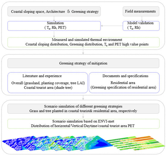
Figure 1.
The study route.
2. Materials and Methods
2.1. Study Area
Qingdao is a coastal city in Eastern China (35°35′–37°09′ N 119°30′–121° E). The average maximum temperature in coastal urban areas in summer is mostly between 24.0 and 30.0 °C, which has been increasing year by year since the 1990s [31]. The southeast wind prevails in summer, and the average wind speed is between 3.4 and 5.4 m/s. The study site is located on a typical urban shoreline, and the sea’s surface is located on the southeast side of the site. The site is divided into two parts: the coastal green area and the residential area. The overall slope is about 4%, and the maximum slope of the coastal green space is 50%. The coastal green area is a local tourist and leisure destination. The green space is densely planted with black pine and a few other trees, with some grass and two large marble paved plazas. Multistory residential buildings with a high building density are located on the sloping land. The height of the buildings in the site is 10–20 m, and the main tree species is black pine (Figure 2). The study site is a typical local urban space with a coastal slope topography, which is representative of the thermal environment.
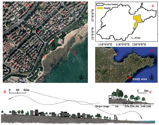
Figure 2.
Schematic diagram of the study area. (a) Geographical location of Qingdao. (b) Location of the study area. (c) Study site: Sea Breeze Square (1–4 is the actual measurement locations). (d) A-A profile. (e) Profile of coastal green space.
2.2. ENVI-Met Model
ENVI-met creates mesh-based 3D models. It evaluates the interactions of the atmosphere, green areas, buildings, and materials with a horizontal and vertical resolution of 0.5–10 m and a time step of 10 s. It can simulate the micro-environmental climate in the urban environment as output. Information about buildings, green areas, and terrain should be inputted into the model. The configuration file includes data on the thermophysical properties of the building materials, meteorological data (wind speed and direction, initial air temperature, humidity, cloudiness, etc.), soil data (initial temperature and humidity at different levels), and the simulation time. Thermal environment studies with ENVI-met require in situ measurements for model validation. Air temperature (Ta) is the most commonly assessed meteorological variable, followed by relative humidity (RH) [32]. Solar radiation (SR) can be matched hourly using the full forcing mode, and it can only be adjusted from the built-in data by an adjustment factor (0.5–1.5) [33,34]. The full forced mode was adopted in this study. Due to the geographical location and summer climate conditions of the study area, the solar radiation was set at 0.5. Wind information (speed and direction) can remain static throughout the simulation time depending on the initial input values [32].
2.3. Field Measurements and Model Validation
Field measurements are required to verify the feasibility of ENVI-met in the study area. Measurements were taken during a typical summer day (4 August 2022). The two consecutive days before this day were sunny. KestrelNK5500 and TES1333R equipment were used to measure the temperature, humidity, wind speed, and solar radiation intensity at a pedestrian height of 1.5 m. We collected data for 10 min before and after each whole period from 7:00 to 20:00, with an automatic recording interval of 30 s. The four measurement locations were on the square, on the grass, in a parking lot, and on the residential (Figure 2). Roadside, terrain, buildings, and greening layout were inputted into the model file. The position and height of the analog data output points were consistent with those of field measurement points. The grid number of the volumetric regular mesh was set to 165*165*25, the horizontal resolution was 4 m, and the vertical resolution was 2 m. Table 1 shows the model’s parameter settings.

Table 1.
Initial settings of the ENVI-met simulation.
In terms of planting, the software provides several plant modeling options, and its parameters can be determined according to the physiological characteristics. The leaf area index (LAI) of typical black pine and ash was measured with a canopy analyzer (LAI-2200). Formula (1) was used to calculate the corresponding LAD at each height of the plant for a given tree height, width, and trunk height (Table 2).
where is the leaf area index, is the leaf area density, is the crown stratification height, and h is the crown height.
Table 2.
Plant model parameters.
According to the measurements and calculation, the final plant model parameters were as shown in Table 2.
The full forcing model was used in the study, and the initial values of the parameters are shown in Table 1. The simulation time was 33 h, and the first 24 h were discarded as the simulation warm-up time.
In the validation results, the temperature in general was slightly lower in the simulated values than the observed values. It can be seen that the simulated values of the coastal square (Point 1) and the grass (Point 2) were close to the observed values, and the change trend was consistent. The simulated values of the green parking lot (Point 3) and the residential undergrowth (Point 4) differed significantly from the observed values, but the trend was generally consistent (Figure 3).
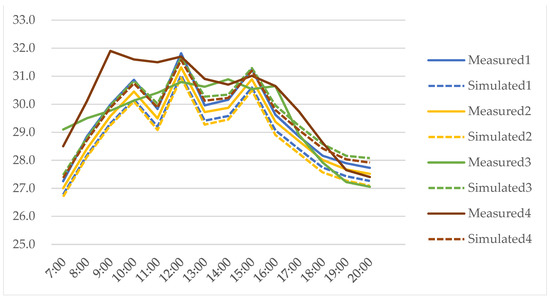
Figure 3.
The hourly mean value of the measured and simulated temperatures of the four measuring points over time.
In terms of humidity, the simulated value was generally slightly higher than the observed value. The simulated values of observation Points 1, 2, and 4 were closer to the observed values, and the trend was consistent. The difference between the simulated and observed values of the green parking lot (Point 3) was more obvious (Figure 4).
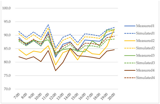
Figure 4.
The hourly mean value of the measured and simulated humidity values of four measuring points over time.
Next, the measured and simulated values of the four points were statistically analyzed. The determination coefficient (R2), the root mean square error (), the systematic root mean square error (), unsystematic root mean square error (), and the index of agreement () were chosen to evaluate the accuracy of the temperature and humidity of the model. R2 is the key coefficient of regression analyses [32]. It is more real and informative than the mean absolute error (MAE), mean squared error (MSE), and RMSE [35]. The explain the part of the total error that always occurs and has specific causes, such as the errors caused by weak characterization of the research object caused by using the meshing method in the ENVI–met model. is composed of input parameters, the accuracy of the constructed model, empirical constants, etc. The index of agreement () is the probability that the simulated value of the model will agree with the measured value. This value indicates how accurately the model predicts a variable, where D = 1 means that the simulated value is completely consistent with the measured value. The formula is as follows [36,37,38]:
where n represents the measured times, is the simulated value, is the measured value, is the simulated average value, is the measured average value, and is the vector of the simulated value.
We quantitatively evaluated the error between the simulated and observed values for temperature and relative humidity (Table 3). The R2 values of all measuring points were greater than 0.6. The d value was greater than 0.89 at all points in terms of temperature. The results showed that the simulated temperature values were in good agreement with the observed values (Table 3). The consistency of humidity was weak. This may be caused by the great change in humidity at the seaside during the measuring days, and the relatively stable change in the ENVI-met simulation. This also explains why the RMSE is generally larger than the RMSEu. According to the analysis of the statistical values of the four measuring points, the simulation values of ENVI-met for the paving sites and grasslands near the seaside were in high agreement with the measured values, and the predictability for the location of parking lots and residential areas was low. This may be because the latter two are close to urban roads and are greatly affected by heat released from vehicle exhausts. ENVI-met cannot simulate the effects of humans, vehicles, and mechanical cooling systems on the thermal environment, which leads to a difference between simulated and observed values. Overall, the simulated temperature’s RMSE values ranged from 0.4 to 1.3 °C and the humidity’s RMSE ranged from 1.7 to 5.3%, which is within the acceptable error range. This indicates that the simulated and measured values had the same trend, and the simulation could predict the changes in the sites’ temperature and humidity better.
Table 3.
Quantitative evaluation of errors of the temperature and humidity (analog values) at four measuring points.
In terms of wind speed, the ENVI-met model used static input to represent the wind speed and direction. Validation studies have shown that ENVI-met has difficulties in predicting the dynamic behavior of one-day spikes [39]. The simulation of dynamic changes in wind speed data was poor, but the wind speed depends mainly on the physical and climatic conditions. Therefore, the changes in wind speed and direction generated by the software simulation reflect the relationship between the site’s status and the climate environment. The simulation data for wind speed are, therefore, of reference value.
2.4. Construction of the Simulation Models
In order to study the mitigating effect of planting on UHI, six scenarios were designed for the coastal green space and the residential area according to different vegetation types and planting patterns. Scenario 1 is the green area with all lawn, and no trees in the residential area. Scenario 2 is a green area with all lawn, and black pine planted in the residential area. In Scenario 3, all areas were planted with black pine. In Scenario 4, all areas were planted with ash. In Scenario 5, the green area was planted with a grass, and the residential area was planted with black pine and additional seaside planting. In Scenario 6, the green area was planted with lawn, and the residential area was planted with ash and additional seaside planting (Figure 5).
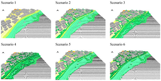
Figure 5.
Models of six planting patterns.
2.5. Statistical Analysis
The effects of different planting patterns on the improvement in the thermal environment and the human thermal comfort index in coastal cities in summer was quantified in this study. Air temperature at pedestrian height is commonly used to assess the urban thermal environment [40]. Air temperature ranges, daily maxima, daily minima, and daily averages are often used to assess the impact of urban form on the thermal environment or to compare the thermal environment of different urban scenarios [41,42]. Therefore, this study uses the air temperature at a pedestrian height of 1.5 m to analyze the urban thermal environment in different scenarios. The evaluation of urban thermal environment should also consider thermal comfort, which is only affected by the air temperature and is also related to other factors, such as relative humidity, wind speed, average radiation temperature, etc. [43]. According to their frequency of use, the human thermal comfort indices include the physiological equivalent temperature (PET), the predicted mean vote (PMV), the universal thermal climate index (UTCI), the comfort formula (COMFA), and the temperature of equivalent perception (TEP). PET is the air temperature at which human skin temperature and body temperature reach a thermal state equivalent to that of a typical indoor environment when located in an indoor or outdoor environment. PET is widely used when assessing the thermal microenvironment [44]. PET adopts the radiant flux from body heat balance in all possible directions and wavelengths, including short-wave and long-wave radiation. Human sex, height, age, weight, heat resistance of clothes, and metabolic heat are included in the calculation. Therefore, PET has become the most widely used index in urban climatology and is considered the most suitable for evaluating outdoor human thermal comfort [45]. PET is a thermal comfort index derived from the Munich energy balance model for individuals (MEMI). The MEMI formula is:
where is the metabolic rate, is the work item, is the radiant heat exchange term, is the convective heat flux, is the heat loss caused by water evaporation to the surrounding air through the surface when the skin is dry, is the sweat heat loss, and is the thermal storage.
In this study, the physiological equivalent temperature (PET) output by the BIO-met module in ENVI–met is taken as the thermal comfort index. To perform PET calculation and analysis, the parameter settings are as follows: height = 1.75 m; weight = 75 kg; age = 35; gender = male; body surface area = 1.91 m2; static clothing insulation index = 0.3; metabolic rate (walking or simple activities) = 86 W·m2.
3. Results and Discussion
3.1. Measured and Simulated Thermal Environment
The following is an analysis of the current thermal environment of the site. According to the field measurement and the data released by the meteorological station, there were three high peaks in the temperature on that day, which were at 10:00, 12:00, and 15:00 hours. Combined with historical meteorological data, the temperature and PET distribution in the site were plotted for 15:00, the highest temperature of the day. Since the site is located on a slope with an altitude of 1–31 m, the method of splicing pedestrian height and the temperature distribution by layers was adopted. The distribution maps at the heights of 2.5, 4.5, 7.5, 10.5, 13.5, 17.5, 20.5, 22.5, 25.5, 28.5, and 32.5 m were extracted for splicing. The following horizontal distribution analyses all used this data selection process. In the current state of the site, the average temperature at pedestrian height was 31.1°C and the average PET is 27.2 °C. The highest and lowest air temperatures were 31.7 °C and 30.4 °C, which were, respectively, located on the urban road at a height of 13.5 m in the residential area and in the coastal green area at a height of 2.5 m near the sea (Figure 6). The highest and lowest temperatures were 33.1 °C and 27.0 °C, respectively, which were located to the north of the buildings at a height of 20 m in the residential area and in the coastal green area at a height of 2.5 m near the sea (Figure 7). It can be seen that the areas with higher air temperatures were distributed in residential locations and were especially concentrated on the urban roads. The distribution of PET was roughly in line with this pattern. PET was lower in areas shaded by trees or buildings, or in the middle of wide urban roads with good ventilation.
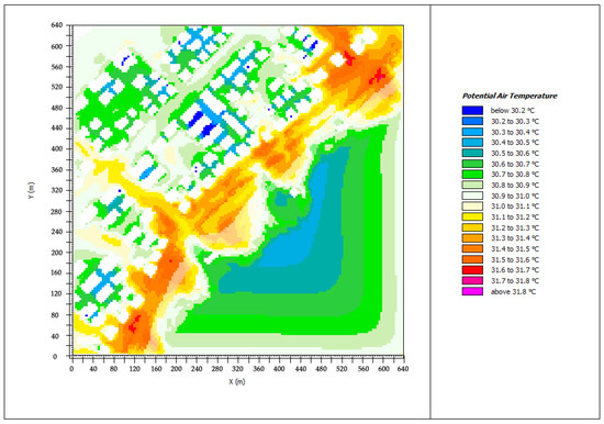
Figure 6.
Temperature distribution at pedestrian height.
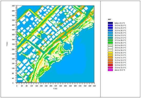
Figure 7.
PET distribution at pedestrian height.
3.2. Temperature Simulations in Six Scenarios
The simulation results of six different planting scenarios showed that plants had an effect on air temperature at 1.5 m height but not significantly (Table S1). In the following analysis, the results of the air temperature simulation at 15:00 are expressed as the average, minimum, and maximum values for the entire study area. The minimum temperature simulated for all scenarios was 30.4 °C, with the highest temperature occurring in Scenario 4, reaching 31.8 °C. The highest average temperature also appears in Scenario 4, reaching 31.2 °C (Table 4). It can be seen that the impact of different planting patterns on the sites’ air temperature was not significant in general, but the impact on the highest temperature was obvious.
Table 4.
Maximum, minimum, and average temperatures for six scenarios.
The simulation results for air temperature at 1.5 m height were divided in increments of 0.3 °C, and the temperature range distribution of each scenario was found. The air temperature of Scenarios 1, 2, 5, and 6 were below 31.5 °C across the region. The proportion of air temperature Scenarios 3 and 4 exceeding 31.5 °C was 0.4% and 2.3%, respectively. In the range below 31.5 °C, the proportion of air temperature in the relatively high range of 30.9–31.5 °C of Scenario 1 to 6 as 86.8%, 85.5%, 94.3%, 84.9%, 92.9, and 94.9%, respectively. In Scenarios 3 and 4, the proportion of high temperature range was significantly higher than that in other scenarios. In particular, the proportion in Scenario 4 was significantly higher than that of other scenarios, both in the relative high temperature range and over 31.5 °C (Figure 8).
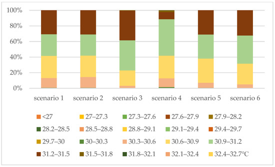
Figure 8.
Temperature range ratios of six scenarios.
3.3. PET Analysis Based on the Simulation Scenarios
3.3.1. Horizontal Distribution of PET
The simulation results of six different planting scenarios (Tables S2 and S3) showed that planting has a great influence on the PET at the height of 1.5 m. The highest and lowest PET in Scenario 1 were the lowest among the six scenarios, followed by Scenario 2. Scenario 4 had the highest average PET and the highest PET of the six scenarios (Table 5), 27.8 °C and 34.3 °C, respectively.
Table 5.
Maximum, minimum, and average PET for six scenarios.
In terms of the percentage of each PET interval, Scenarios 1 and 2 were had a significantly higher percentage below 27 °C than Scenarios 3–6, reaching 98.5% and 98.7%, respectively. In the other four scenarios, temperatures lower than 27 °C accounted for 50–82.2%. For temperatures in the range of 27–28.5 °C, the proportions for Scenarios 3–6 were 32.5%, 32.2%, 14.6%, and 26.5%, respectively. The proportions of temperatures in the higher PET interval above 31.2 °C in Scenarios 3–6 were 3%, 7.7%, 0.7%, and 3.7%, respectively. The proportions of temperatures in the PET range below 27.3 °C in Scenarios 1, 2, and 5 were 98.7%, 98.9%, and 91.2%, respectively, and those of Scenarios 3, 4, and 6 were 72%, 56.8% and 81.3%, respectively. Overall, Scenario 1 and 2 achieved the best PET effect, followed by Scenario 5 (Figure 9).
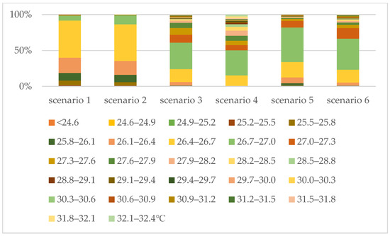
Figure 9.
PET range ratios of six scenarios.
The above results show that Scenario 1 without trees had the lowest PET, and that of Scenario 2 with shade trees planted in residential areas according to the greening specification was slightly higher than that of Scenario 1. In Scenarios 3–6, for the highest and average values of PET as well as the low temperature range, the order from low to high was: Scenario 5 < Scenario 3 < Scenario 6 < Scenario 4. This shows that trees can increase PET in the coastal area, and the higher the LAI, the more obvious the warming effect.
By visualizing the PET simulation results in the plan view, the PET distribution of each scenario can be seen. The highest PETs in Scenario 1 and Scenario 2 were the same. These occurred in the coastal green space, which is located on the shady side of a 10.5 m building, reaching 28.3 °C and 28.5 °C, respectively. The highest PET in Scenario 3 occurred in the residential area, which is located outside the area with street trees at the back of a building with a height of 32.5 m near the road, reaching 32.3 °C. The highest PET in Scenario 4 occurred in the residential area, between the shady side of a 22.5 m high building and the street trees, and near the urban trunk road, reaching 34.3 °C. The highest temperature of PET in Scenario 5 occurred in the residential area, which is located on the shady side of a 32.5-m-high building and also outside the area of street trees near the urban road, reaching 31.7 °C. The highest temperature of PET in Scenario 6 occurred in the residential area, between the shady side of a 25.5-m-high building and the street trees, and close to the urban trunk road, reaching 33.1 °C. In addition, from the PET plane distribution map, the different planting patterns made the distribution of PET above the sea surface different for each scenario. In Scenario 1 and 2, when there were no trees in the coastal green space, the area with a PET below 26.5 °C above the sea surface was larger. In Scenarios 3–6, the area with a low temperature above the sea surface in Scenario 5 was the largest and that of Scenario 4 was the smallest. These results show that the highest PET at pedestrian height appeared in the gap between the shady side of the buildings and the trees along the urban trunk road. In addition, according to the plane distribution of PET, with an increase in tree area or LAI under the same tree coverage, the cool area formed above the sea becomes smaller (Figure 10).
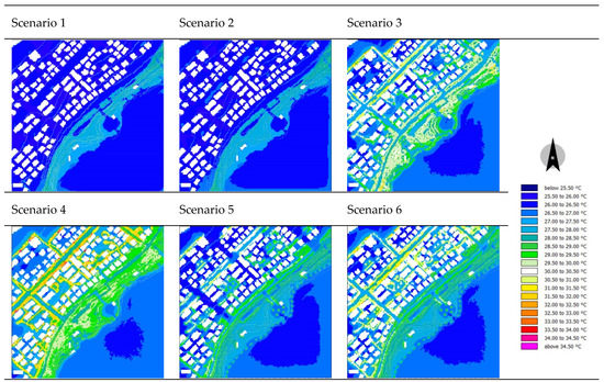
Figure 10.
PET at pedestrian height at 15:00.
A scatter plot was drawn for the average PET in the interval of the aforementioned height position according to different simulation scenarios (Figure 11), where the abscissa was the average distance between the site and the shoreline. It should be noted that the 120 m distance from the coastline is basically the boundary between coastal green space and residential area in the study area. As a large number of buildings in the residential area would have a great impact on the thermal environment, the site was divided into two parts to analysis: coastal green space and residential area. In the coastal green space, that is, within the range of less than 120 m from the coastline, the PET of all scenarios increased with the increase of distance. In residential areas, the PET in Scenario 1 tended to decrease with increasing distance from the coastline. The PET in Scenario 2 was almost the same, but there was a lift at the distance of 350 m. The PET in Scenario 3 and 5 showed a rising-falling-rising-falling state with 200 m and 350 m as the boundary. The PET in Scenarios 4 and 6 showed a trend of rising first and then falling with 350 m as the boundary. This showed that the ocean has obvious cooling effect in the urban space of coastal slope topography. However, under the combined action of topography, elevation and planting, this cooling effect had a certain range of action. Overall, the PET increased with increasing distance from the shoreline in coastal green areas, whether lawns or trees were planted. In the residential area, with 350 m as the boundary, the PET showed a trend of rising first and then falling.
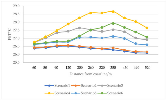
Figure 11.
Average PET at different distances from the coastline.
3.3.2. Vertical Distribution of PET
The east–west section of the highest PET position at 15:00 in the six scenarios is shown in Figure 10. The x value in the illustration is the abscissa of the maximum PET value, and the h value is the ordinate. Figure 12a,b shows that the highest PET in Scenarios 1 and 2 was in the same position. The location is in a coastal green space with a building shield less than 5 m above the sea breeze, and its rear topographic slope is nearly 50%. In both scenarios, the overall vertical distribution of low PET values formed by the buildings in the residential area was not very different, but in Scenario 2 with street trees, the area of high PET near the ground formed by the buildings and trees together was larger than that in Scenario 1. Figure 12c shows that the highest PET in Scenario 3 was located at 32.5 m in the shade of a building with flat terrain behind it, adjacent to the city road. Figure 12d shows that the highest PET in Scenario 4 occurred to the back of a 22.5 m building, which was under a dense tree canopy and adjacent to the road. Figure 12e shows the highest PET in Scenario 5 at 32.5 m, which was located to the back of a building, with a topographic slope to the rear of about 8%. Figure 12f shows that the highest PET in Scenario 6 was located at 25.5 m in the shade behind a building with a rearward terrain slope of about 12%.
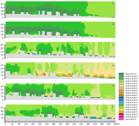
Figure 12.
The x–z profile of the highest PET position: (a) Scenario 1: h = 10.5 m, x = 508 m; (b) Scenario 2: h = 10.5 m, x = 508 m; (c) Scenario 3: h = 32.5 m, x = 72m; (d) Scenario 4: h = 22.5 m, x = 228 m; (e) Scenario 5: h = 32.5 m, x = 36 m; (f) Scenario 6: h = 25.5 m, x = 200 m.
These results indicate that a high PET at pedestrian height is more often found in the angle formed by the shady rear side of a building and the sloping ground. Above pedestrian height, a low-PET zone formed above the buildings in all six scenarios, and this low-PET zone decreased and fragmented with increased tree planting or LAI.
3.3.3. Daytime Distribution of PET
The average PET for the six scenarios from 7:00 to 18:00 was also analyzed in this study. According to the statistical data here, we can see that Scenarios 1 and 2 had the lowest average PET at each statistical time node during the day. The average PET of Scenario 1 was higher than that of Scenario 2 before 11:00, but vice versa after 12:00. The average daily PET of the other four scenarios showed a consistent change rule. Overall, the order of PET from low to high was Scenario 5 < Scenario 6 < Scenario 3 < Scenario 4 (Figure 13). Scenario 4 was significantly higher than other scenarios in terms of the distribution of the average PET throughout the day.
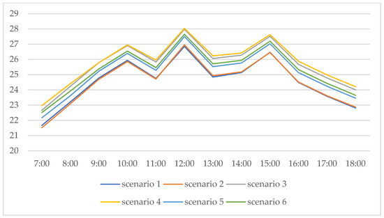
Figure 13.
Average PET at 07:00–18:00.
This ranking is consistent with the previous analysis of the high and low PET values at 15:00. This indicates that the results of the analysis are highly representative. At the same time, the comparison between Scenarios 1 and 2 also show that tree planting may create a certain cooling effect in the morning.
3.3.4. PET of the Coastal Tourist Area
The coastal tourist area in this study had the urban characteristics of a typical local tourist areas, and tourists are mostly concentrated in the promenade and square in this coastal area. Therefore, the following PET analysis focused on the coastal central square to form a planting strategy for the coastal tourist area. Taking the pavement site in the coastal green space as the area for calculation, the daily average PET values of Scenarios 1–6 were 24.54 °C, 24.53 °C, 25.64 °C, 25.79 °C, 25.11 °C, and 25.31 °C, respectively. The average PET values at 15:00 during the hottest period in the afternoon were 26.49 °C, 26.46 °C, 27.51 °C, 27.62 °C, 27.03 °C, and 27.19 °C, respectively. According to the PET of the coastal tourism area, Scenarios 1 and 2 had the best cooling effect, while Scenario 4 was the worst. According to the distribution of daytime PET from 7:00 to 18:00, Scenario 4 was the highest for almost all time points. In a comparison between Scenarios 1 and 2, Scenario 1 was slightly higher than Scenario 2 before 11:00, and vice versa afterwards. The trend of Scenarios 4–6 tended to be consistent and, overall, Scenario 5 was slightly lower (Figure 14).
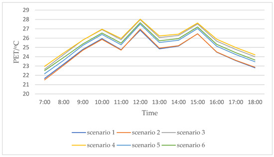
Figure 14.
Coastal tourist area’s PET at 7:00–18:00.
The ranking of PET comfort in the coastal excursion area was consistent with the results of the previous domain-wide study, which indicated that the factors influencing temperature in the coastal excursion area are the same as in the entire study domain. However, in the coastal tourist area, the difference in PET between Scenario 4 and the other scenarios was smaller. This indicates that the effect of planting on the site’s PET was not as strong at the seaside as in the residential area.
To show the vertical distribution of PET in the coastal tourist area, Figure 15 depicts the east–west profile of the coastal central square. The horizontal range of 388–456 m in the figure is the central square area. The PET distribution in this area is described below. It can be seen that the pedestrian height in the square area in Figure 15a,b is in the low and homogeneous PET range, about 26–26.1 °C. Figure 15c,d also shows a relatively low PET distribution in this region, between 26.5 °C and 26.8 °C for Scenario 3 and between 26.7 °C and 27.2 °C for Scenario 4. Figure 15a–d shows that if there is a slope facing the sea breeze in the square area, this can produce a low temperature area at pedestrian height, and the closer to the ground and the center of the square, the lower the PET. When planted on slopes, the cooling effect of lawns is better than that of trees. With an increase in the LAI of trees, the warming effect on the square may be enhanced. Figure 15e,f show that the square’s PET range in Scenario 5 was 26.6–28.9 °C and that in Scenario 6 was 26.7–29.2 °C. Hotter areas are generated below the canopy. Therefore, planting trees in the square will produce a local high PET under the canopy, and the higher the tree LAI, the more obvious the warming effect.
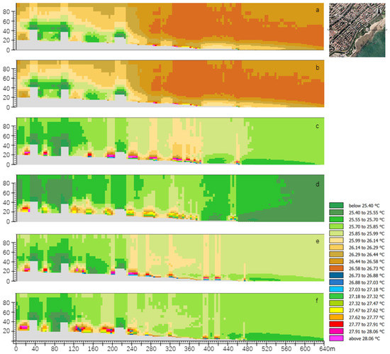
Figure 15.
PET profile of central square location at 15:00: (a) Scenario 1; (b) Scenario 2; (c) Scenario 3; (d) Scenario 4; (e) Scenario 5; (f) Scenario 6.
3.4. Discussion
In terms of the spatial distribution of PET in a coastal urban green space, the closer to the seaside, the better the thermal comfort that can be obtained. The high heat capacity and low thermal conductivity of water create a “constant temperature effect”; that is to say, it can significantly reduce the sensible change in heat of the city [46]. Sea breezes and land breezes dominate the wind patterns of coastal cities during the day and at night [47]. Sea breezes can reduce daytime and nighttime air temperatures without obstacles [9]. This is consistent with the results of this study. However, some studies have shown that although the evaporation of water will reduce temperature, it will also increase humidity, thus reducing thermal comfort [48]. The influence of humidity on PET was beyond the scope of this study, but this conclusion may explain the negative impact of planting on PET in coastal areas in this study. The distribution of PET in the residential area was more complicated. The PET decreased with the increase of elevation when there were no trees in the current coastal green space. The PET showed a trend of rising first and then falling with the boundary of 21 m elevation and 350 m from the coastline when there were trees planted in coastal green space. The increase of PET was most likely related to the cooling of the ocean. The part of PET reduction might be related to the gradient wind blowing from the ocean direction. Gradient wind is a phenomenon in which wind speed increases proportionally to vertical height. With the increased of elevation, the gradient wind speed in urban space increased, and the corresponding PET decreased [49]. This was consistent with the results of this study.
Planting trees increased the PET of the site, and the higher the LAI of the trees, the more obvious the warming effect. This may be due to the dependence of the research site on the cooling effect of sea breezes. Most studies believe that plants usually affect the physical environment of cities through transpiration and shadowing effects, selective absorption, and reflection of thermal radiation, so that they have cooling effects [50,51]. This seems to be contrary to the conclusion of this study. However, it can be seen from the vertical analysis of this study that the sea breezes were blocked by the tree crown, forming a high PET zone under the tree. This shows that the cooling effect of sea breezes plays a decisive role in this research site. This is consistent with the conclusion of some studies that the cooling intensity of water is stronger than that of green space [50,52]. Therefore, in this study, because the dense tree planting blocked the sea breeze at pedestrian height, the cooling effect was reduced, which led to the phenomenon of plant warming. At the same time, the area of high humidity under the canopy may be caused by the evaporation and transpiration of plants. The combined effect of an area of calm air and high humidity may explain why the PET under the tree crown was higher in the square with tree planting, and PET was positively correlated with LAI.
In terms of pedestrian height, the area where the buildings face the sea breeze tend to have higher PET, especially when there is a sloping terrain behind it or when there are densely planted street trees on an urban trunk road. This may be caused by the combined action of the area of calm air formed by building shielding and thermal radiation from the surface.
The study discussed the thermal environment of urban space under the joint action of an ocean, sloping terrain, buildings, and plants. Only a few studies have researched urban greening strategies with a similar geographical environment at the city scale through land surface temperature inversion before. This study has made a more detailed exploration on the microscale, making up for the lack of research in this area. In addition, we have also drawn some conclusions that can form a framework for studies researching another coastal area with flat terrain in the same city. In the future, the results can be used to form a systematic greening strategy for coastal cities.
Due to the measurement conditions, this study failed to conduct nighttime measurement. Therefore, ENVI-met validation and a simulation analysis were not conducted for nighttime conditions. Because of the constant temperature characteristics of water bodies, these usually have a nocturnal warming effect on the surrounding area. Plants have a cooling effect at night [53]. Therefore, in terms of the overall effect of coastal cities on alleviating the urban heat island effect, it is necessary to increase nighttime analyses. It is hoped that there will be an opportunity to include nocturnal measurements and analyses when the scientific research conditions permit, so as to provide more complete research results.
4. Conclusions
The study showed that, in the coastal urban green space with a sloping terrain, the closer to the seaside, the better the thermal comfort. At 15:00, during the hottest period of the day in summer, the cooling effect of lawns is better than that of trees, and trees with a low LAI were better than those with high LAI. On the coastal slope terrain, the high PET at pedestrian height easily appeared at the angle between the shady facade of buildings and the terrain or close to the trees on the side of urban trunk roads. A negative impact on thermal comfort would be generated by increasing the planting of trees for shading in coastal tourist areas.
According to the results of actual measurements and the design scenario simulation, the following greening strategies can be suggested.
Planting street trees on urban roads can have the effect of reducing PET.
The cooling effect of lawns is better than that of trees. The lower the LAI of planted trees, the lower the site’s PET.
With the aim of meeting the greening standards of residential area, lawn planting should be carried out in coastal green spaces, and trees with low LAI should be selected in residential areas.
If the distance between the tree crown and a building’s shady facade is too close, it can easily produce high PET, so the tree crown should be kept away from the building shady facade.
The planting of tree areas on the coastal walkway or the square will improve the local PET. Trees should not be planted on the seashore roads nor the square to keep the sea breeze unblocked.
Supplementary Materials
The following supporting information can be downloaded at: https://www.mdpi.com/article/10.3390/su15010295/s1, Table S1: Temperature of six scenarios; Table S2: PET of six scenarios; Table S3: Measuring Data; Model S1–S6: Scenario model.
Author Contributions
Conceptualization, Y.Z. and X.H.; methodology, Y.Z.; software, Y.Z.; validation, Y.Z., Z.L. and H.L.; formal analysis, Y.Z.; investigation, Z.L.; resources, C.Z.; data curation, Y.Z.; writing—original draft preparation, Y.Z.; writing—review and editing, Y.Z.; visualization, Z.L.; supervision, X.H.; project administration, Y.Z.; funding acquisition, X.H. All authors have read and agreed to the published version of the manuscript.
Funding
This work was supported by the Key Disciplines of State Forestry Administration of China (No. 21 of Forest Ren Fa, 2016); Hunan Province “Double First-class” Cultivation discipline of China (No. 469 of Xiang Jiao Tong, 2018).
Institutional Review Board Statement
Not applicable.
Informed Consent Statement
Not applicable.
Data Availability Statement
The data that support the findings of this study are available from the author upon reasonable request.
Conflicts of Interest
The authors declare no conflict of interest.
References
- Williams, S.; Nitschke, M.; Weinstein, P.; Pisaniello, D.L.; Parton, K.A.; Bi, P. The impact of summer temperatures and heatwaves on mortality and morbidity in Perth, Australia 1994–2008. Environ. Int. 2012, 40, 33–38. [Google Scholar] [CrossRef] [PubMed]
- Zhang, Y.; Nitschke, M.; Bi, P. Risk factors for direct heat-related hospitalization during the 2009 Adelaide heatwave: A case crossover study. Sci. Total. Environ. 2013, 442, 1–5. [Google Scholar] [CrossRef] [PubMed]
- Jamei, E.; Rajagopalan, P.; Seyedmahmoudian, M.; Jamei, Y. Review on the impact of urban geometry and pedestrian level greening on outdoor thermal comfort. Renew. Sustain. Energy Rev. 2016, 54, 1002–1017. [Google Scholar] [CrossRef]
- Santamouris, M.; Synnefa, A.; Karlessi, T. Using advanced cool materials in the urban built environment to mitigate heat islands and improve thermal comfort conditions. Sol. Energy 2011, 85, 3085–3102. [Google Scholar] [CrossRef]
- Lai, D.; Liu, W.; Gan, T.; Liu, K.; Chen, Q. A review of mitigating strategies to improve the thermal environment and thermal comfort in urban outdoor spaces. Sci. Total. Environ. 2019, 661, 337–353. [Google Scholar] [CrossRef]
- Tablada, A.; De Troyer, F.; Blocken, B.; Carmeliet, J.; Verschure, H. On natural ventilation and thermal comfort in compact urban environments—The Old Havana case. Build. Environ. 2009, 44, 1943–1958. [Google Scholar] [CrossRef]
- Ziter, C.D.; Pedersen, E.J.; Kucharik, C.J.; Turner, M.D. Scale-dependent interactions between tree canopy cover and impervious surfaces reduce daytime urban heat during summer. Proc. Natl. Acad. Sci. USA 2019, 116, 7575–7580. [Google Scholar] [CrossRef]
- Bettio, L.; Nairn, J.R.; McGibbony, S.C.; Hope, P.; Tupper, A.; Fawcett, R.J.B. A heatwave forecast service for Australia. Proc. R. Soc. Vic. 2019, 131, 53–59. [Google Scholar] [CrossRef]
- Zhou, X.; Okaze, T.; Ren, C.; Cai, M.; Ishida, Y.; Watanabe, H.; Mochida, A. Evaluation of urban heat islands using local climate zones and the influence of sea-land breeze. Sustain. Cities Soc. 2020, 55, 102060. [Google Scholar] [CrossRef]
- Saburo, M.; Sekine, T.; Narita, K.; Nishina, D. Study of the effects of a river on the thermal environment in an urban area. Energy Build. 1991, 16, 993–1001. [Google Scholar]
- Oke, T.R. City size and the urban heat island. Atmos. Environ. 1973, 7, 769–779. [Google Scholar] [CrossRef]
- Theeuwes, N.E.; Solcerová, A.; Steeneveld, G.J. Modeling the influence of open water surfaces on the summertime temperature and thermal comfort in the city. J. Geophys. Res. Atmos. 2013, 118, 8881–8896. [Google Scholar] [CrossRef]
- Völker, S.; Kistemann, T. Developing the urban blue: Comparative health responses to blue and green urban open spaces in Germany. Health Place 2015, 35, 196–205. [Google Scholar] [CrossRef] [PubMed]
- Montazeri, H.; Toparlar, Y.; Blocken, B.; Hensen, J. Simulating the cooling effects of water spray systems in urban landscapes: A computational fluid dynamics study in Rotterdam, The Netherlands. Landsc. Urban Plan. 2017, 159, 85–100. [Google Scholar] [CrossRef]
- Du, H.; Song, X.; Jiang, H.; Kan, Z.; Wang, Z.; Cai, Y. Research on the cooling island effects of water body: A case study of Shanghai, China. Ecol. Indic. 2016, 67, 31–38. [Google Scholar] [CrossRef]
- Yang, G.; Yu, Z.; Jørgensen, G.; Vejre, H. How can urban blue-green space be planned for climate adaption in high-latitude cities? A seasonal perspective. Sustain. Cities Soc. 2020, 53, 101932. [Google Scholar] [CrossRef]
- Sun, R.; Chen, L. How can urban water bodies be designed for climate adaptation? Landsc. Urban Plan. 2012, 105, 27–33. [Google Scholar] [CrossRef]
- Žuvela-Aloise, M.; Koch, R.; Buchholz, S.; Früh, B. Modelling the potential of green and blue infrastructure to reduce urban heat load in the city of Vienna. Clim. Chang. 2016, 135, 425–438. [Google Scholar] [CrossRef]
- Ren, Y.; Deng, L.-Y.; Zuo, S.-D.; Song, X.-D.; Liao, Y.-L.; Xu, C.-D.; Chen, Q.; Hua, L.-Z.; Li, Z.-W. Quantifying the influences of various ecological factors on land surface temperature of urban forests. Environ. Pollut. 2016, 216, 519–529. [Google Scholar] [CrossRef]
- Taleghani, M. Outdoor thermal comfort by different heat mitigation strategies—A review. Renew. Sustain. Energy Rev. 2018, 81, 2011–2018. [Google Scholar] [CrossRef]
- Taha, H. Cool Cities: Counteracting Potential Climate Change and its Health Impacts. Curr. Clim. Chang. Rep. 2015, 1, 163–175. [Google Scholar] [CrossRef]
- Monteiro, M.V.; Doick, K.J.; Handley, P.; Peace, A. The impact of greenspace size on the extent of local nocturnal air temperature cooling in London. Urban For. Urban Green. 2016, 16, 160–169. [Google Scholar] [CrossRef]
- Hardin, P.J.; Jensen, R.R. The effect of urban leaf area on summertime urban surface kinetic temperatures: A Terre Haute case study. Urban For. Urban Green. 2007, 6, 63–72. [Google Scholar] [CrossRef]
- Qiu, G.Y.; Zou, Z.; Li, X.; Li, H.; Guo, Q.; Yan, C.; Tan, S. Experimental studies on the effects of green space and evapotranspiration on urban heat island in a subtropical megacity in China. Habitat Int. 2017, 68, 30–42. [Google Scholar] [CrossRef]
- Ren, C.; Yang, R.; Cheng, C.; Xing, P.; Fang, X.; Zhang, S.; Wang, H.; Shi, Y.; Zhang, X.; Kwok, Y.T.; et al. Creating breathing cities by adopting urban ventilation assessment and wind corridor plan—The implementation in Chinese cities. J. Wind. Eng. Ind. Aerodyn. 2018, 182, 170–188. [Google Scholar] [CrossRef]
- Zhang, Y.; Hu, X.; Cao, X.; Liu, Z. Numerical Simulation of the Thermal Environment during Summer in Coastal Open Space and Research on Evaluating the Cooling Effect: A Case Study of May Fourth Square, Qingdao. Sustainability 2022, 14, 15126. [Google Scholar] [CrossRef]
- Xiao, J.; Yuizono, T. Climate-adaptive landscape design: Microclimate and thermal comfort regulation of station square in the Hokuriku Region, Japan. Build. Environ. 2022, 212, 108813. [Google Scholar] [CrossRef]
- Yang, Y.; Gatto, E.; Gao, Z.; Buccolieri, R.; Morakinyo, T.E.; Lan, H. The “plant evaluation model” for the assessment of the impact of vegetation on outdoor microclimate in the urban environment. Build. Environ. 2019, 159, 106151. [Google Scholar] [CrossRef]
- Morakinyo, T.E.; Kong, L.; Lau, K.K.-L.; Yuan, C.; Ng, E. A study on the impact of shadow-cast and tree species on in-canyon and neighborhood’s thermal comfort. Build. Environ. 2017, 115, 1–17. [Google Scholar] [CrossRef]
- Koc, C.B.; Osmond, P.; Peters, A. Evaluating the cooling effects of green infrastructure: A systematic review of methods, indicators and data sources. Sol. Energy 2018, 166, 486–508. [Google Scholar] [CrossRef]
- Tian, Y.; Ma, Y.; Dong, H.; Guo, L. Analysis of climatic and environmental characteristics in Qingdao under the background of climate change. Trans. Oceanol. Limnol. 2012, 04, 10–15. [Google Scholar]
- Liu, Z.; Cheng, W.; Jim, C.; Morakinyo, T.E.; Shi, Y.; Ng, E. Heat mitigation benefits of urban green and blue infrastructures: A systematic review of modeling techniques, validation and scenario simulation in ENVI-met V4. Build. Environ. 2021, 200, 107939. [Google Scholar] [CrossRef]
- Liu, Z.; Zheng, S.; Zhao, L. Evaluation of the ENVI-Met Vegetation Model of Four Common Tree Species in a Subtropical Hot-Humid Area. Atmosphere 2018, 9, 198. [Google Scholar] [CrossRef]
- Acero, J.A.; Herranz-Pascual, K. A comparison of thermal comfort conditions in four urban spaces by means of measurements and modelling techniques. Build. Environ. 2015, 93, 245–257. [Google Scholar] [CrossRef]
- Chicco, D.; Warrens, M.J.; Jurman, G. The coefficient of determination R-squared is more informative than SMAPE, MAE, MAPE, MSE and RMSE in regression analysis evaluation. PeerJ Comput. Sci. 2021, 7, e623. [Google Scholar] [CrossRef] [PubMed]
- Fox, D.G. Judging Air Quality Model Performance. Bull. Am. Meteorol. Soc. 1981, 62, 599–609. [Google Scholar] [CrossRef]
- Willmott, C.J. Some Comments on the Evaluation of Model Performance. Bull. Am. Meteorol. Soc. 1982, 63, 1309–1313. [Google Scholar] [CrossRef]
- Stunder, M.; Sethuraman, S. A statistical evaluation and comparison of coastal point source Dispersion Models. Atmos. Environ. 1986, 20, 301–315. [Google Scholar] [CrossRef]
- Forouzandeh, A. Numerical modeling validation for the microclimate thermal condition of semi-closed courtyard spaces between buildings. Sustain. Cities Soc. 2018, 36, 327–345. [Google Scholar] [CrossRef]
- Tong, S.; Wong, N.H.; Jusuf, S.K.; Tan, C.L.; Wong, H.F.; Ignatius, M.; Tan, E. Study on correlation between air temperature and urban morphology parameters in built environment in northern China. Build. Environ. 2018, 127, 239–249. [Google Scholar] [CrossRef]
- Xu, D.; Zhou, D.; Wang, Y.; Xu, W.; Yang, Y. Field measurement study on the impacts of urban spatial indicators on urban climate in a Chinese basin and static-wind city. Build. Environ. 2019, 147, 482–494. [Google Scholar] [CrossRef]
- Perini, K.; Magliocco, A. Effects of vegetation, urban density, building height, and atmospheric conditions on local temperatures and thermal comfort. Urban For. Urban Green. 2014, 13, 495–506. [Google Scholar] [CrossRef]
- Lai, D.; Lian, Z.; Liu, W.; Guo, C.; Liu, W.; Liu, K.; Chen, Q. A comprehensive review of thermal comfort studies in urban open spaces. Sci. Total. Environ. 2020, 742, 140092. [Google Scholar] [CrossRef] [PubMed]
- Höppe, P.R. Heat balance modelling. Experientia 1993, 49, 741–746. [Google Scholar] [CrossRef] [PubMed]
- Fang, Z.; Feng, X.; Liu, J.; Lin, Z.; Mak, C.M.; Niu, J.; Tse, K.-T.; Xu, X. Investigation into the differences among several outdoor thermal comfort indices against field survey in subtropics. Sustain. Cities Soc. 2018, 44, 676–690. [Google Scholar] [CrossRef]
- Oke, T.R. Boundary Layer Climates; Routledge: London, UK; New York, NY, USA, 2002. [Google Scholar]
- Zhong, S.; Takle, E.S. An Observational Study of Sea- and Land-Breeze Circulation in an Area of Complex Coastal Heating. J. Appl. Meteorol. 1992, 31, 1426–1438. [Google Scholar] [CrossRef]
- Wu, Y.; Hai, G.; Hao, S. Impacts of urban cooling effect based on landscape scale: A review. Natl. Cent. Biotechnol. Inf. 2015, 26, 636–642. [Google Scholar]
- Sihong, D.; Zhang, X.; Jin, X.; Zhou, X.; Shi, X. A review of multi-scale modelling, assessment, and improvement methods of the urban thermal and wind environment. Build. Environ. 2022, 213, 108860. [Google Scholar]
- Bowler, D.E.; Buyung-Ali, L.; Knight, T.M.; Pullin, A.S. Urban greening to cool towns and cities: A systematic review of the empirical evidence. Landsc. Urban Plan. 2010, 97, 147–155. [Google Scholar] [CrossRef]
- Wong, N.H.; Yu, C. Study of green areas and urban heat island in a tropical city. Habitat Int. 2005, 29, 547–558. [Google Scholar] [CrossRef]
- Lin, W.; Yu, T.; Chang, X.; Wu, W.; Zhang, Y. Calculating cooling extents of green parks using remote sensing: Method and test. Landsc. Urban Plan. 2015, 134, 66–75. [Google Scholar] [CrossRef]
- Kaaviya, P.U.; Ramalingam, S. A review of the impact of the green landscape interventions on the urban microclimate of tropical areas. Build. Environ. 2021, 205, 108190. [Google Scholar]


Disclaimer/Publisher’s Note: The statements, opinions and data contained in all publications are solely those of the individual author(s) and contributor(s) and not of MDPI and/or the editor(s). MDPI and/or the editor(s) disclaim responsibility for any injury to people or property resulting from any ideas, methods, instructions or products referred to in the content. |
© 2022 by the authors. Licensee MDPI, Basel, Switzerland. This article is an open access article distributed under the terms and conditions of the Creative Commons Attribution (CC BY) license (https://creativecommons.org/licenses/by/4.0/).