
An Accurate Model for Bifacial Photovoltaic Panels

 , , , and
Abstract
:1. Introduction
1.1. General
1.2. Literature Review
1.3. Article Contributions
- An improved modeling method of BPV modules is proposed in this paper. The proposed method adapts the module’s series resistance to effectively describe the performance of BPV modules in the full operating range whilst considering the nonlinear properties of BPV systems. Thence, this paper introduces new modeling for BPV modules, which has seen little coverage in the literature.
- A generalized method is proposed to determine the unified model parameters to describe the BPV for the whole operating front-side and back-side irradiance levels. The proposed method represents a two-step optimization method for modeling BPV systems. Compared to existing methods in the literature, the proposed method has high precision for modeling both MPV operation and BPV operation.
- An enhanced application of the powerful LSHADE optimizer is introduced for determining the optimum model parameters of BPV using SDM and DDM. The LSHADE method is advantageous at adapting the internal parameters of the algorithm based on the acquired knowledge along evolutionary processes with the continuous reduction of populations.
2. SDM and DDM for PV Modules
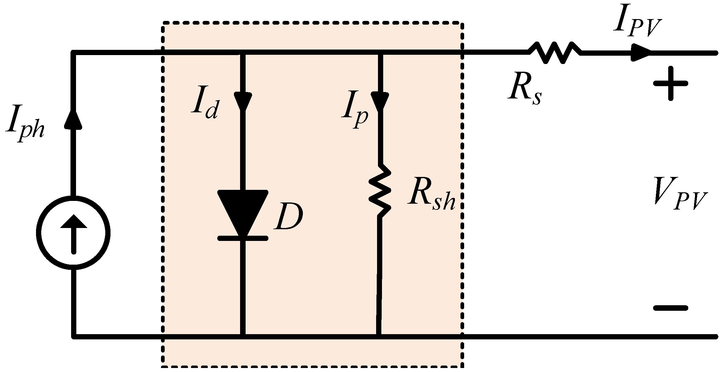
2.1. The SDM-Based Modeling
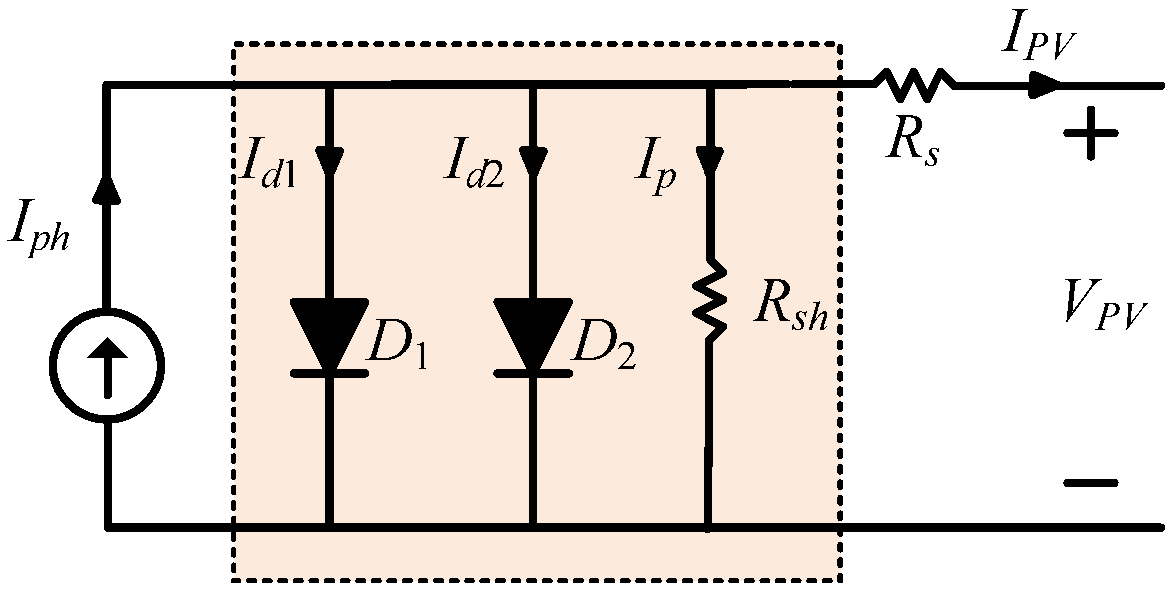
2.2. The DDM-Based Modeling
3. Formulation of the Optimization Problem
3.1. For SDM Model
3.2. For DDM Model
4. The Proposed Modified Method for BPV Modeling
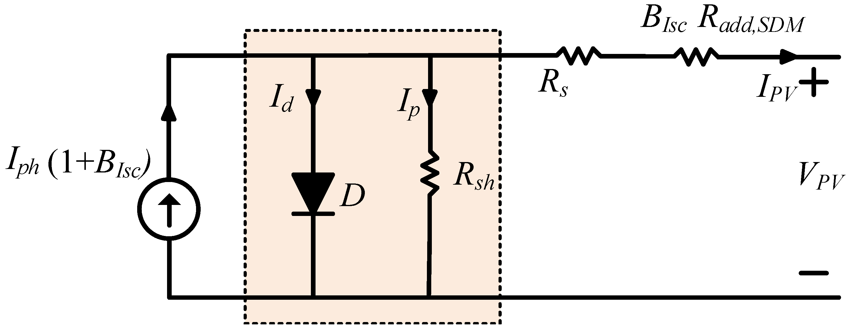
4.1. For SDM Model
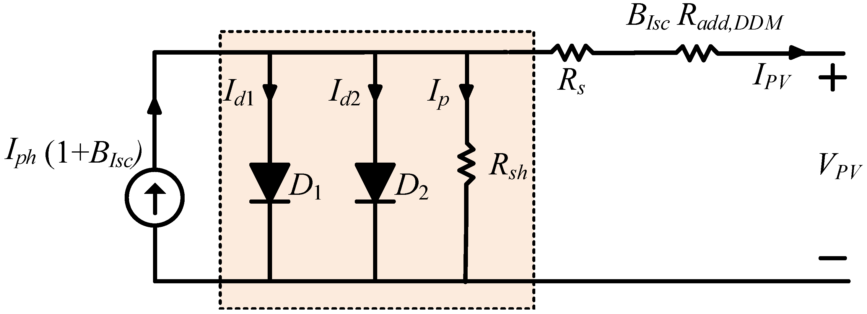
4.2. For DDM Model
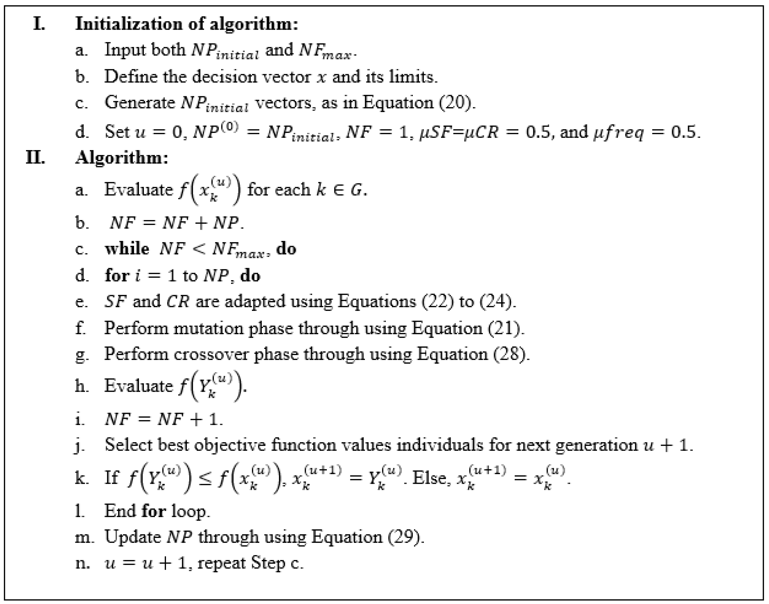
5. The Proposed LSHADE Method
5.1. Initialization Step
5.2. Mutation Step
5.3. Adaptation of Parameter Step
5.4. Crossover
5.5. Population Reduction Stage
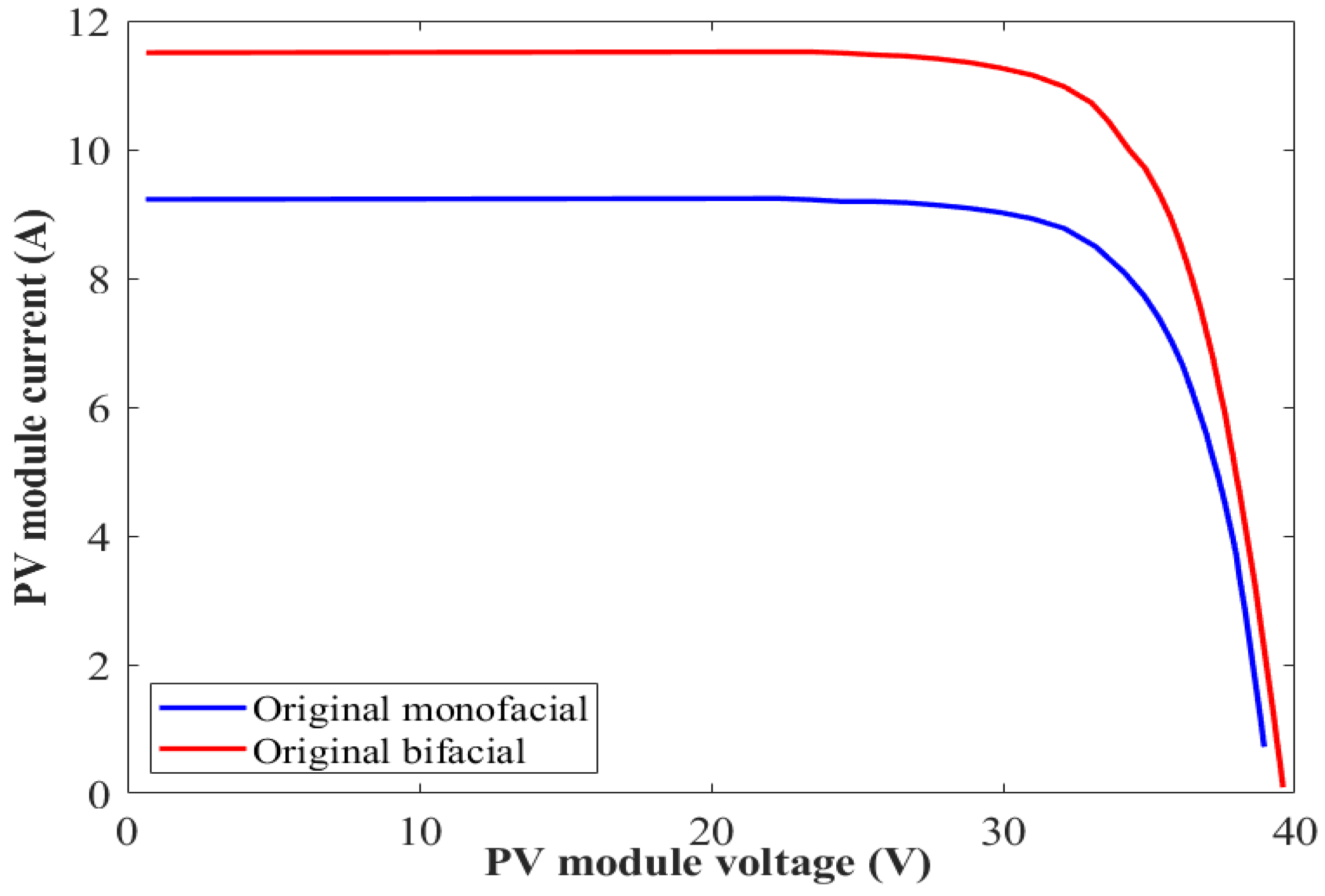
6. Results and Discussion
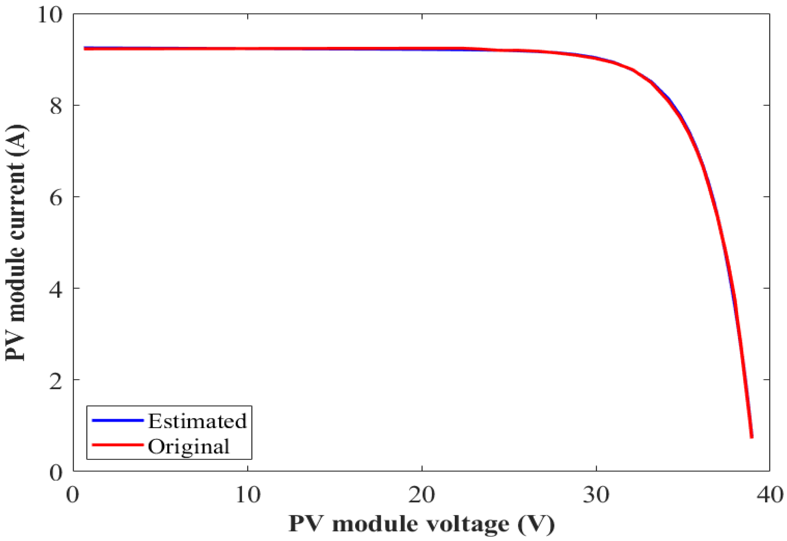
6.1. Results for SDM of BPV Module
6.2. Results for DDM of BPV Module
7. Performance Comparisons of LSHADE Method
8. Conclusions
- The proposed method is advantageous in terms of model accuracy and precisely modeling both the MPV and BPV.
- In addition, the proposed method is general and can be applied to the various single- and double-diode models of bifacial PV systems.
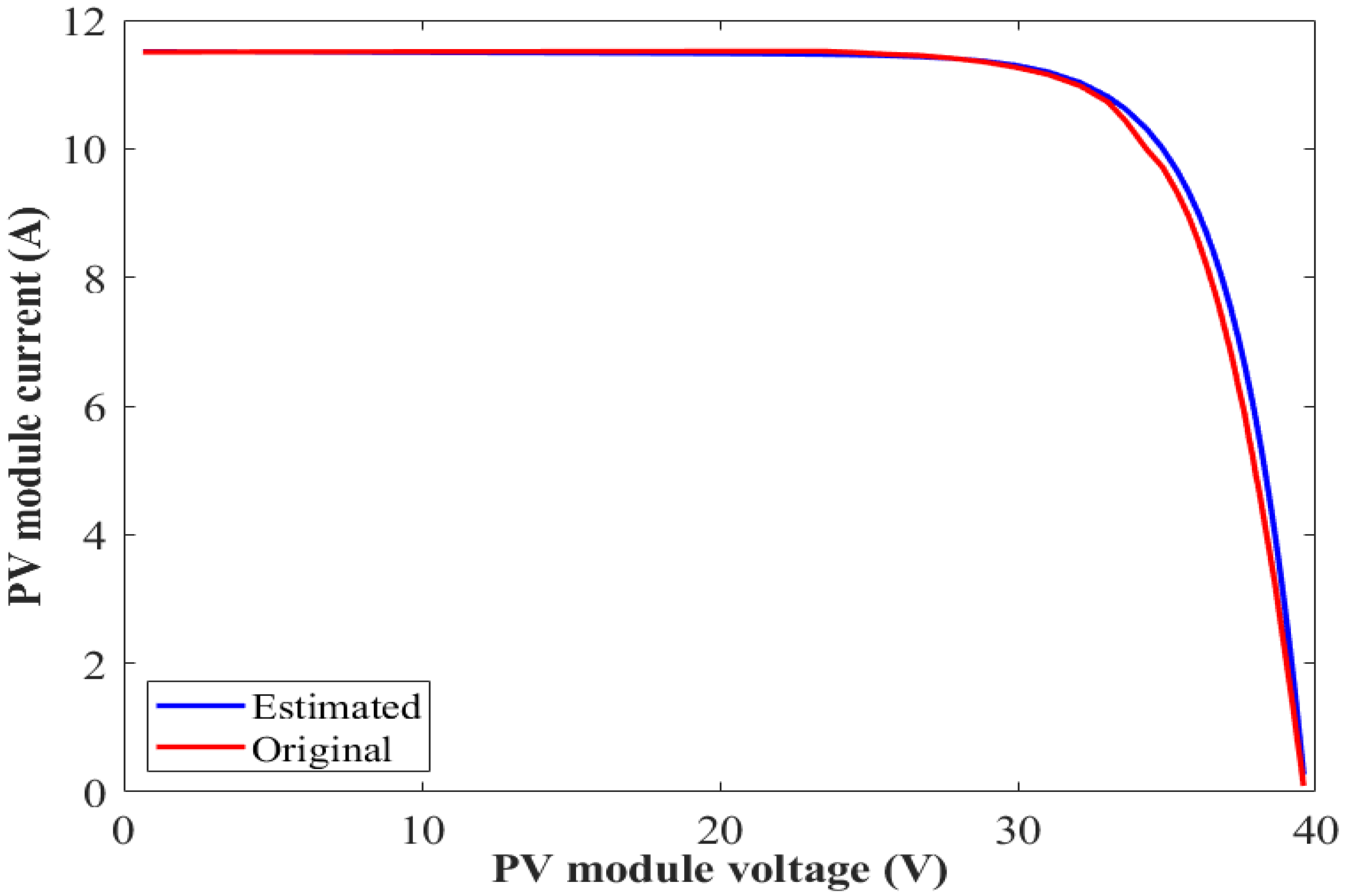
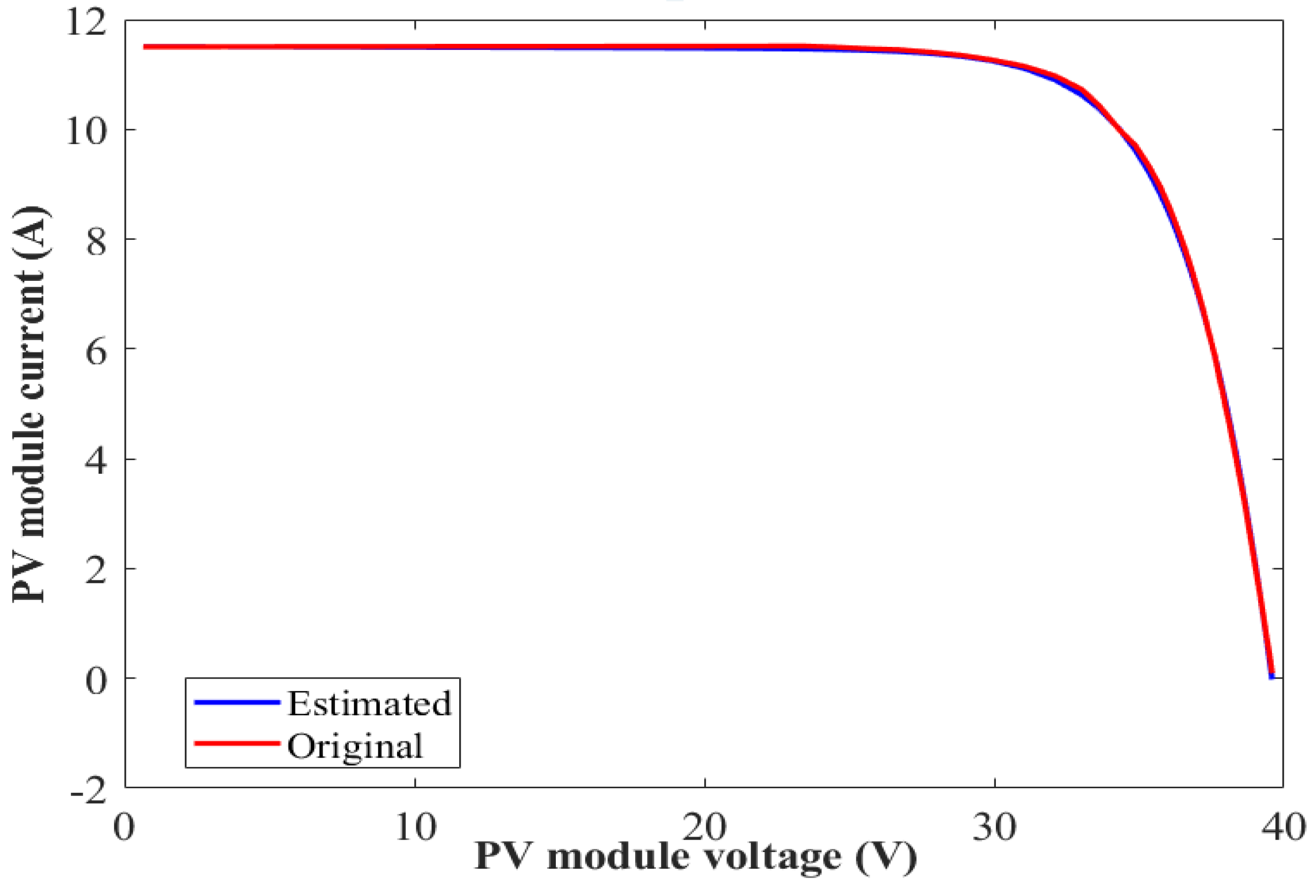
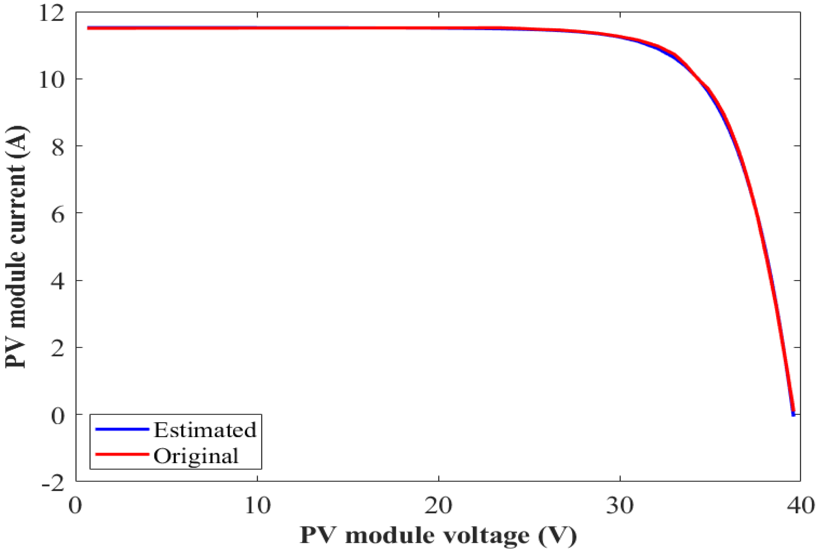
- The proposed method achieves the RMSE values of 0.0538 and 0.0530 compared to 0.4519 and 0.4621 under the conventional method for SDM and DDM, respectively.
- The proposed method has MAE values of 0.0435 and 0.0396 compared to 0.3125 and 0.3143 under the conventional method for SDM and DDM, respectively.
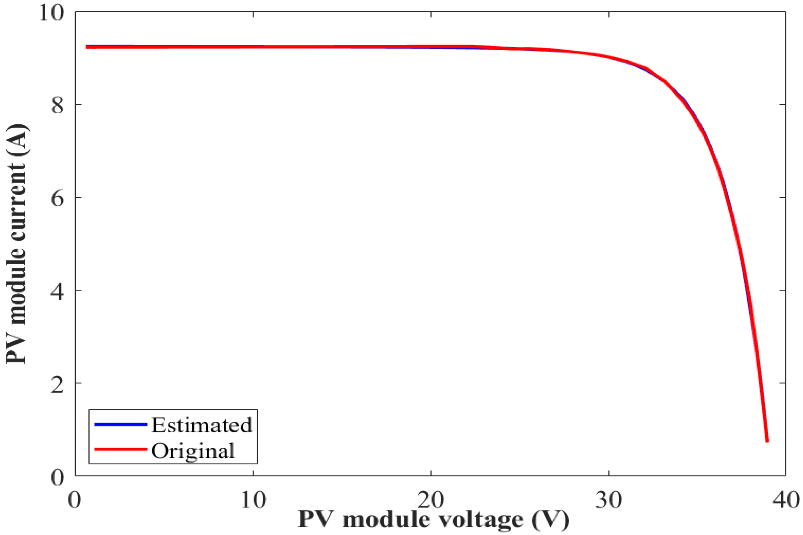
- The obtained results show the effectiveness and the accuracy of the proposed method with a reduced error in the obtained representations for both the SDM and DDM of BPV modules.
Author Contributions
Funding
Institutional Review Board Statement
Informed Consent Statement
Data Availability Statement
Conflicts of Interest
Nomenclature
| PV Models | |
| The ideality factors of , respectively | |
| The bifaciality factor of the short circuit current | |
| The reverse-saturation current in , respectively | |
| The currents in diodes , respectively | |
| Photo-electric current | |
| The model external outputted current | |
| The current of | |
| K | Boltzman constant |
| The number of series-connected cells in the module | |
| Set of parameters of DDM of BPV modules | |
| Set of parameters of DDM of MPV modules | |
| Set of parameters of SDM of BPV modules | |
| Set of parameters of SDM of MPV modules | |
| q | The electron charge |
| The series added resistance to DDM to compensate for the nonlinearity of the BPV systems. | |
| The series added resistance to SDM to compensate for the nonlinearity of the BPV systems. | |
| The model parallel resistance | |
| The model series resistance | |
| T | The junction temperature |
| The terminal voltage of model | |
| The thermal voltage | |
| The LSHADE Algorithm | |
| The total number of iterations | |
| The number of variables | |
| The present number of objective function evaluations | |
| The maximum number of objective function evaluations | |
| The initial population size | |
| The scaling factor | |
| The lower limit of each variable of searching range | |
| The upper limit of each variable of searching range | |
| The best individual in the current generation u | |
| RMSE | Root mean-square error |
| RMSE | Root mean-square error |
References
- Aboagye, B.; Gyamfi, S.; Ofosu, E.A.; Djordjevic, S. Investigation into the impacts of design, installation, operation and maintenance issues on performance and degradation of installed solar photovoltaic (PV) systems. Energy Sustain. Dev. 2022, 66, 165–176. [Google Scholar] [CrossRef]
- Rezk, H.; Abdelkareem, M.A. Optimal parameter identification of triple diode model for solar photovoltaic panel and cells. Energy Rep. 2022, 8, 1179–1188. [Google Scholar] [CrossRef]
- Al-Janahi, S.A.; Ellabban, O.; Al-Ghamdi, S.G. Technoeconomic feasibility study of grid-connected building-integrated photovoltaics system for clean electrification: A case study of Doha metro. Energy Rep. 2020, 6, 407–414. [Google Scholar] [CrossRef]
- Berrian, D.; Libal, J.; Klenk, M.; Nussbaumer, H.; Kopecek, R. Performance of Bifacial PV Arrays With Fixed Tilt and Horizontal Single-Axis Tracking: Comparison of Simulated and Measured Data. IEEE J. Photovoltaics 2019, 9, 1583–1589. [Google Scholar] [CrossRef]
- Mostafa, M.; Rezk, H.; Aly, M.; Ahmed, E.M. A new strategy based on slime mould algorithm to extract the optimal model parameters of solar PV panel. Sustain. Energy Technol. Assess. 2020, 42, 100849. [Google Scholar] [CrossRef]
- Molin, E.; Stridh, B.; Molin, A.; Wäckelgård, E. Experimental Yield Study of Bifacial PV Modules in Nordic Conditions. IEEE J. Photovoltaics 2018, 8, 1457–1463. [Google Scholar] [CrossRef]
- Pelaez, S.A.; Deline, C.; Greenberg, P.; Stein, J.S.; Kostuk, R.K. Model and Validation of Single-Axis Tracking with Bifacial PV. IEEE J. Photovoltaics 2019, 9, 715–721. [Google Scholar] [CrossRef]
- Raina, G.; Sinha, S. A comprehensive assessment of electrical performance and mismatch losses in bifacial PV module under different front and rear side shading scenarios. Energy Convers. Manag. 2022, 261, 115668. [Google Scholar] [CrossRef]
- Zhao, O.; Zhang, W.; Xie, L.; Wang, W.; Chen, M.; Li, Z.; Li, J.; Wu, X.; Zeng, X.; Du, S. Investigation of indoor environment and thermal comfort of building installed with bifacial PV modules. Sustain. Cities Soc. 2022, 76, 103463. [Google Scholar] [CrossRef]
- Tina, G.M.; Bontempo Scavo, F.; Merlo, L.; Bizzarri, F. Comparative analysis of monofacial and bifacial photovoltaic modules for floating power plants. Appl. Energy 2021, 281, 116084. [Google Scholar] [CrossRef]
- Ayadi, O.; Jamra, M.; Jaber, A.; Ahmad, L.; Alnaqep, M. An Experimental Comparison of Bifacial and Monofacial PV Modules. In Proceedings of the 2021 12th International Renewable Engineering Conference (IREC), Amman, Jordan, 14–15 April 2021; pp. 1–8. [Google Scholar] [CrossRef]
- Muehleisen, W.; Loeschnig, J.; Feichtner, M.; Burgers, A.; Bende, E.; Zamini, S.; Yerasimou, Y.; Kosel, J.; Hirschl, C.; Georghiou, G. Energy yield measurement of an elevated PV system on a white flat roof and a performance comparison of monofacial and bifacial modules. Renew. Energy 2021, 170, 613–619. [Google Scholar] [CrossRef]
- Nussbaumer, H.; Klenk, M.; Morf, M.; Keller, N. Energy yield prediction of a bifacial PV system with a miniaturized test array. Sol. Energy 2019, 179, 316–325. [Google Scholar] [CrossRef]
- Narvarte, L.; Almeida, R.; Carrêlo, I.; Rodríguez, L.; Carrasco, L.; Martinez-Moreno, F. On the number of PV modules in series for large-power irrigation systems. Energy Convers. Manag. 2019, 186, 516–525. [Google Scholar] [CrossRef]
- Ahmed, E.M.; Aly, M.; Elmelegi, A.; Alharbi, A.G.; Ali, Z.M. Multifunctional Distributed MPPT Controller for 3P4W Grid-Connected PV Systems in Distribution Network with Unbalanced Loads. Energies 2019, 12, 4799. [Google Scholar] [CrossRef] [Green Version]
- Tahir, F.; Baloch, A.A.; Al-Ghamdi, S.G. Impact of climate change on solar monofacial and bifacial Photovoltaics (PV) potential in Qatar. Energy Rep. 2022, 8, 518–522. [Google Scholar] [CrossRef]
- Jain, P.; Raina, G.; Mathur, S.; Sinha, S. Optical Modeling Techniques for Bifacial PV. In Renewable Energy for Sustainable Growth Assessment; John Wiley & Sons, Ltd.: Hobohen, NJ, USA, 2022; Chapter 7, pp. 181–215. [Google Scholar] [CrossRef]
- Tina, G.M.; Scavo, F.B.; Aneli, S.; Gagliano, A. Assessment of the electrical and thermal performances of building integrated bifacial photovoltaic modules. J. Clean. Prod. 2021, 313, 127906. [Google Scholar] [CrossRef]
- Lorenzo, E. On the historical origins of bifacial PV modelling. Sol. Energy 2021, 218, 587–595. [Google Scholar] [CrossRef]
- Ghenai, C.; Ahmad, F.F.; Rejeb, O.; Bettayeb, M. Artificial neural networks for power output forecasting from bifacial solar PV system with enhanced building roof surface Albedo. J. Build. Eng. 2022, 56, 104799. [Google Scholar] [CrossRef]
- Wang, L.; Tang, Y.; Zhang, S.; Wang, F.; Wang, J. Energy yield analysis of different bifacial PV (photovoltaic) technologies: TOPCon, HJT, PERC in Hainan. Sol. Energy 2022, 238, 258–263. [Google Scholar] [CrossRef]
- Yin, H.; Zhou, Y.; Sun, S.; Tang, W.; Shan, W.; Huang, X.; Shen, X. Optical enhanced effects on the electrical performance and energy yield of bifacial PV modules. Sol. Energy 2021, 217, 245–252. [Google Scholar] [CrossRef]
- Jiang, F.; He, K. Electrical performance test of N-type bifacial photovoltaic module. In Proceedings of the 2020 Chinese Control and Decision Conference (CCDC), Hefei, China, 22–24 August 2020; pp. 1351–1354. [Google Scholar] [CrossRef]
- Bhang, B.G.; Lee, W.; Kim, G.G.; Choi, J.H.; Park, S.Y.; Ahn, H.K. Power Performance of Bifacial c-Si PV Modules With Different Shading Ratios. IEEE J. Photovoltaics 2019, 9, 1413–1420. [Google Scholar] [CrossRef]
- Zhang, Y.; Yu, Y.; Meng, F.; Liu, Z. Experimental Investigation of the Shading and Mismatch Effects on the Performance of Bifacial Photovoltaic Modules. IEEE J. Photovoltaics 2020, 10, 296–305. [Google Scholar] [CrossRef]
- Silva, E.A.; Bradaschia, F.; Cavalcanti, M.C.; Nascimento, A.J.; Michels, L.; Pietta, L.P. An Eight-Parameter Adaptive Model for the Single Diode Equivalent Circuit Based on the Photovoltaic Module’s Physics. IEEE J. Photovoltaics 2017, 7, 1115–1123. [Google Scholar] [CrossRef]
- Gu, W.; Li, S.; Liu, X.; Chen, Z.; Zhang, X.; Ma, T. Experimental investigation of the bifacial photovoltaic module under real conditions. Renew. Energy 2021, 173, 1111–1122. [Google Scholar] [CrossRef]
- Moshksar, E.; Ghanbari, T. Adaptive Estimation Approach for Parameter Identification of Photovoltaic Modules. IEEE J. Photovoltaics 2017, 7, 614–623. [Google Scholar] [CrossRef]
- Yeh, W.C.; Huang, C.L.; Lin, P.; Chen, Z.; Jiang, Y.; Sun, B. Simplex simplified swarm optimisation for the efficient optimisation of parameter identification for solar cell models. IET Renew. Power Gener. 2018, 12, 45–51. [Google Scholar] [CrossRef]
- Batzelis, E.I.; Papathanassiou, S.A. A Method for the Analytical Extraction of the Single-Diode PV Model Parameters. IEEE Trans. Sustain. Energy 2016, 7, 504–512. [Google Scholar] [CrossRef]
- Batzelis, E.I. Simple PV Performance Equations Theoretically Well Founded on the Single-Diode Model. IEEE J. Photovoltaics 2017, 7, 1400–1409. [Google Scholar] [CrossRef]
- Piazza, M.C.D.; Luna, M.; Petrone, G.; Spagnuolo, G. Translation of the Single-Diode PV Model Parameters Identified by Using Explicit Formulas. IEEE J. Photovoltaics 2017, 7, 1009–1016. [Google Scholar] [CrossRef]
- Nunes, H.; Pombo, J.; Bento, P.; Mariano, S.; Calado, M. Collaborative swarm intelligence to estimate PV parameters. Energy Convers. Manag. 2019, 185, 866–890. [Google Scholar] [CrossRef]
- Awadallah, M.A.; Venkatesh, B. Bacterial Foraging Algorithm Guided by Particle Swarm Optimization for Parameter Identification of Photovoltaic Modules. Can. J. Electr. Comput. Eng. 2016, 39, 150–157. [Google Scholar] [CrossRef]
- Fathy, A.; Elaziz, M.A.; Sayed, E.T.; Olabi, A.; Rezk, H. Optimal parameter identification of triple-junction photovoltaic panel based on enhanced moth search algorithm. Energy 2019, 188, 116025. [Google Scholar] [CrossRef]
- Mahmoud, Y.; El-Saadany, E.F. A Photovoltaic Model With Reduced Computational Time. IEEE Trans. Ind. Electron. 2015, 62, 3534–3544. [Google Scholar] [CrossRef]
- Muhammad, F.F.; Sangawi, A.W.K.; Hashim, S.; Ghoshal, S.K.; Abdullah, I.K.; Hameed, S.S. Simple and efficient estimation of photovoltaic cells and modules parameters using approximation and correction technique. PLoS ONE 2019, 14, e0216201. [Google Scholar] [CrossRef] [PubMed] [Green Version]
- Kler, D.; Sharma, P.; Banerjee, A.; Rana, K.; Kumar, V. PV cell and module efficient parameters estimation using Evaporation Rate based Water Cycle Algorithm. Swarm Evol. Comput. 2017, 35, 93–110. [Google Scholar] [CrossRef]
- Zhang, H.; Heidari, A.A.; Wang, M.; Zhang, L.; Chen, H.; Li, C. Orthogonal Nelder-Mead moth flame method for parameters identification of photovoltaic modules. Energy Convers. Manag. 2020, 211, 112764. [Google Scholar] [CrossRef]
- Ibrahim, I.A.; Hossain, M.J.; Duck, B.C.; Fell, C.J. An Adaptive Wind-Driven Optimization Algorithm for Extracting the Parameters of a Single-Diode PV Cell Model. IEEE Trans. Sustain. Energy 2020, 11, 1054–1066. [Google Scholar] [CrossRef]
- Subudhi, B.; Pradhan, R. Bacterial Foraging Optimization Approach to Parameter Extraction of a Photovoltaic Module. IEEE Trans. Sustain. Energy 2018, 9, 381–389. [Google Scholar] [CrossRef]
- Yu, K.; Liang, J.; Qu, B.; Chen, X.; Wang, H. Parameters identification of photovoltaic models using an improved JAYA optimization algorithm. Energy Convers. Manag. 2017, 150, 742–753. [Google Scholar] [CrossRef]
- Houssein, E.H.; Nassef, A.M.; Fathy, A.; Mahdy, M.A.; Rezk, H. Modified search and rescue optimization algorithm for identifying the optimal parameters of high efficiency triple-junction solar cell/module. Int. J. Energy Res. 2022, 46, 13961–13985. [Google Scholar] [CrossRef]
- Zaky, A.A.; Fathy, A.; Rezk, H.; Gkini, K.; Falaras, P.; Abaza, A. A Modified Triple-Diode Model Parameters Identification for Perovskite Solar Cells via Nature-Inspired Search Optimization Algorithms. Sustainability 2021, 13, 12969. [Google Scholar] [CrossRef]
- Yousri, D.; Shaker, Y.; Mirjalili, S.; Allam, D. An efficient photovoltaic modeling using an Adaptive Fractional-order Archimedes Optimization Algorithm: Validation with partial shading conditions. Solar Energy 2022, 236, 26–50. [Google Scholar] [CrossRef]
- Rezk, H.; Babu, T.S.; Al-Dhaifallah, M.; Ziedan, H.A. A robust parameter estimation approach based on stochastic fractal search optimization algorithm applied to solar PV parameters. Energy Rep. 2021, 7, 620–640. [Google Scholar] [CrossRef]
- Elaziz, M.A.; Almodfer, R.; Ahmadianfar, I.; Ibrahim, I.A.; Mudhsh, M.; Abualigah, L.; Lu, S.; El-Latif, A.A.A.; Yousri, D. Static models for implementing photovoltaic panels characteristics under various environmental conditions using improved gradient-based optimizer. Sustain. Energy Technol. Assessments 2022, 52, 102150. [Google Scholar] [CrossRef]
- Silfab’s Bifacial 360 Ultra-High-Efficiency Modules. Technical Datasheet SLG-X 360 Wp, Silfab, 2021. Available online: https://silfabsolar.com/slg-x-360/ (accessed on 6 November 2022).
- Raya-Armenta, J.M.; Ortega, P.R.; Bazmohammadi, N.; Spataru, S.V.; Vasquez, J.C.; Guerrero, J.M. An Accurate Physical Model for PV Modules With Improved Approximations of Series-Shunt Resistances. IEEE J. Photovoltaics 2021, 11, 699–707. [Google Scholar] [CrossRef]
- Hachana, O.; Aoufi, B.; Tina, G.M.; Sid, M.A. Photovoltaic mono and bifacial module/string electrical model parameters identification and validation based on a new differential evolution bee colony optimizer. Energy Convers. Manag. 2021, 248, 114667. [Google Scholar] [CrossRef]
- Storn, R.; Price, K. Differential evolution—A simple and efficient heuristic for global optimization over continuous spaces. J. Glob. Optim. 1997, 11, 341–359. [Google Scholar] [CrossRef]
- Tanabe, R.; Fukunaga, A. Success-history based parameter adaptation for Differential Evolution. In Proceedings of the 2013 IEEE Congress on Evolutionary Computation, Cancun, Mexico, 20–23 June 2013. [Google Scholar] [CrossRef] [Green Version]
- Awad, N.H.; Ali, M.Z.; Suganthan, P.N.; Reynolds, R.G. An ensemble sinusoidal parameter adaptation incorporated with L-SHADE for solving CEC2014 benchmark problems. In Proceedings of the 2016 IEEE Congress on Evolutionary Computation (CEC), Vancouver, BC, Canada, 24–29 July 2016. [Google Scholar] [CrossRef]
- Fathy, A.; Aleem, S.H.E.A.; Rezk, H. A novel approach for PEM fuel cell parameter estimation using LSHADE - EpSin optimization algorithm. Int. J. Energy Res. 2021, 45, 6922–6942. [Google Scholar] [CrossRef]


| Electrical | STC at | STC at Front + Irradiance % on Back Side | NOCT at | |||
|---|---|---|---|---|---|---|
| Specifications | Front | 15% | 20% | 25% | 30% | Front |
| (W) | 360.0 | 405.9 | 421.2 | 436.5 | 451.9 | 274.5 |
| (A) | 8.9 | 9.95 | 10.33 | 10.68 | 11.04 | 6.8 |
| (V) | 40.3 | 39.44 | 39.46 | 39.52 | 39.53 | 40.3 |
| (A) | 9.7 | 10.57 | 10.98 | 11.38 | 11.77 | 7.7 |
| (V) | 47. | 5 47.81 | 47.86 | 47.90 | 47.98 | 47.0 |
| Efficiency | 18.46% | 20.24% | 21.60% | 22.38% | 23.17% | 17.6% |
| Parameter | Boundary | Optimal Parameters (DDM) Conventional | Proposed | |||
|---|---|---|---|---|---|---|
| Min. | Max. | MPV Only | BPV Only | Scaling MPV | Method | |
| (A) | 0.0 | 12 | 9.2464 | 11.5113 | 9.2464 | 9.2464 |
| (A) | ||||||
| a | 0.0 | 3.0 | 1.2280 | 1.1664 | 1.2280 | 1.2280 |
| 0.0 | 5000 | 661.2200 | 4705.3 | 661.2200 | 661.2200 | |
| 0.0 | 1.0 | 0.01 | 0.0754 | 0.01 | 0.01 | |
| 0.0 | 1.0 | — | — | — | 0.39 | |
| 0.0321 | 0.0345 | 0.4519 | 0.0538 | |||
| 0.0236 | 0.0259 | 0.3125 | 0.0435 | |||
| 0.9999 | 0.9999 | 0.9858 | 0.9998 | |||
| Parameter | Boundary | Optimal Parameters (DDM) Conventional | Proposed | |||
|---|---|---|---|---|---|---|
| Min. | Max. | MPV Only | BPV Only | Scaling MPV | Method | |
| (A) | 0.0 | 12 | 9.2379 | 11.5232 | 9.2379 | 9.2379 |
| (A) | ||||||
| (A) | ||||||
| 0.0 | 3.0 | 2.3665 | 2.4942 | 2.3665 | 2.3665 | |
| 0.0 | 3.0 | 1.1738 | 1.2178 | 1.1738 | 1.1738 | |
| 0.0 | 5000 | 4488.9748 | 4348.9552 | 4488.9748 | 4488.9748 | |
| 0.0 | 1.0 | 0.01 | 0.0629 | 0.01 | 0.01 | |
| 0.0 | 1.0 | — | — | — | 0.41 | |
| 0.0279 | 0.0427 | 0.4621 | 0.0530 | |||
| 0.0191 | 0.0323 | 0.3143 | 0.0396 | |||
| 0.9999 | 0.9999 | 0.9852 | 0.9998 | |||
| Run No. | LSHADE | SCA | AEO | ASO | SMA | MPA |
|---|---|---|---|---|---|---|
| 1 | 0.031301782 | 0.347265266 | 0.029924963 | 0.166870224 | 0.039802333 | 0.045475419 |
| 2 | 0.045984225 | 0.24030415 | 0.046179282 | 0.063442297 | 0.040931443 | 0.050654598 |
| 3 | 0.029802696 | 0.466750656 | 0.051108826 | 0.191040182 | 0.053404346 | 0.0467553 |
| 4 | 0.035614495 | 0.296088206 | 0.041756257 | 0.250520982 | 0.029934247 | 0.030048178 |
| 5 | 0.032802254 | 1.057749553 | 0.041832899 | 0.180936404 | 0.119548975 | 0.049326078 |
| 6 | 0.029511653 | 0.391723026 | 0.037515532 | 0.075012915 | 0.057295955 | 0.061429031 |
| 7 | 0.032339831 | 0.381258343 | 0.040422073 | 0.098276595 | 0.045873362 | 0.030357461 |
| 8 | 0.036047852 | 0.750971209 | 0.033204699 | 0.125610159 | 0.06117019 | 0.062945774 |
| 9 | 0.074731026 | 1.20277875 | 0.052478552 | 0.145481508 | 0.049403854 | 0.046329233 |
| 10 | 0.035976252 | 0.224309244 | 0.038183257 | 0.154148555 | 0.140792614 | 0.082601218 |
| 11 | 0.029629578 | 0.740312706 | 0.032829873 | 0.234284739 | 0.05388134 | 0.04635604 |
| 12 | 0.033848511 | 0.531043584 | 0.032043539 | 0.147601301 | 0.056233513 | 0.036072274 |
| 13 | 0.03603033 | 0.449658834 | 0.03040842 | 0.222619863 | 0.084209319 | 0.100400849 |
| 14 | 0.031229036 | 0.470646191 | 0.029435805 | 0.109929286 | 0.201742478 | 0.091687324 |
| 15 | 0.02933224 | 0.672743035 | 0.042047279 | 0.050210287 | 0.085406166 | 0.04548336 |
| 16 | 0.032110862 | 0.904973735 | 0.040845861 | 0.194559707 | 0.088988915 | 0.041790774 |
| 17 | 0.030198193 | 0.26228278 | 0.040616418 | 0.198487163 | 0.075866397 | 0.114174565 |
| 18 | 0.029618632 | 0.346358068 | 0.040736633 | 0.100026198 | 0.056941617 | 0.04408729 |
| 19 | 0.032846288 | 0.518007716 | 0.032301602 | 0.149009044 | 0.065389952 | 0.037144361 |
| 20 | 0.029487126 | 0.382742771 | 0.032709624 | 0.109345045 | 0.196806016 | 0.054565684 |
| 21 | 0.031792066 | 0.340719384 | 0.032855151 | 0.120429719 | 0.041650539 | 0.036442765 |
| 22 | 0.029675494 | 0.428000437 | 0.033792674 | 0.104403584 | 0.043391312 | 0.055121835 |
| 23 | 0.029587059 | 0.271264182 | 0.04967191 | 0.111079526 | 0.055018014 | 0.029865091 |
| 24 | 0.031958269 | 0.474475342 | 0.031990669 | 0.207917859 | 0.031257339 | 0.033222618 |
| 25 | 0.046578843 | 0.371585699 | 0.050241951 | 0.070425603 | 0.102030862 | 0.097472745 |
| 26 | 0.038340429 | 0.622467131 | 0.034101394 | 0.197425253 | 0.091590727 | 0.075567015 |
| 27 | 0.038326347 | 0.314203704 | 0.035322589 | 0.165007498 | 0.071699543 | 0.086275356 |
| 28 | 0.037019875 | 0.686659217 | 0.039293975 | 0.175400184 | 0.161269555 | 0.050266469 |
| 29 | 0.033515796 | 0.472381055 | 0.04029131 | 0.12853282 | 0.076445682 | 0.042383453 |
| 30 | 0.037207863 | 0.462041639 | 0.029658382 | 0.078324976 | 0.033063702 | 0.063550457 |
| AVG | 0.035081497 | 0.50272552 | 0.038126713 | 0.144211983 | 0.077034677 | 0.056261754 |
| MEDIAN | 0.032571043 | 0.455850236 | 0.037849394 | 0.146541405 | 0.059233072 | 0.048040689 |
| STD | 0.008713375 | 0.237788143 | 0.006768953 | 0.053741309 | 0.045578528 | 0.022960587 |
| Best | 0.02933224 | 0.224309244 | 0.029435805 | 0.050210287 | 0.029934247 | 0.029865091 |
| Worst | 0.074731026 | 1.20277875 | 0.052478552 | 0.250520982 | 0.201742478 | 0.114174565 |
| Run No. | LSHADE | SCA | AEO | ASO | SMA | MPA |
|---|---|---|---|---|---|---|
| 1 | 0.034189644 | 1.15038179 | 0.070227853 | 0.212619162 | 0.17526472 | 0.054383022 |
| 2 | 0.075608676 | 0.607142681 | 0.041205081 | 0.182964487 | 0.059772625 | 0.048403619 |
| 3 | 0.029375189 | 0.79847023 | 0.032489498 | 0.119831767 | 0.089395072 | 0.056169344 |
| 4 | 0.029972137 | 0.587178015 | 0.031385305 | 0.194920938 | 0.034786902 | 0.078303381 |
| 5 | 0.057890571 | 0.671252247 | 0.052218187 | 0.201460221 | 0.129323623 | 0.032842401 |
| 6 | 0.029431209 | 0.639823702 | 0.038841115 | 0.149651521 | 0.092778928 | 0.049020376 |
| 7 | 0.031359129 | 0.41687846 | 0.051115721 | 0.161138388 | 0.138624157 | 0.045564405 |
| 8 | 0.029713905 | 0.53164077 | 0.050408847 | 0.164832292 | 0.05143026 | 0.054441371 |
| 9 | 0.03484947 | 0.269608415 | 0.03421572 | 0.150982301 | 0.062980588 | 0.052784859 |
| 10 | 0.031794089 | 0.29843143 | 0.053907787 | 0.201369713 | 0.045888967 | 0.113319899 |
| 11 | 0.036144978 | 1.100389227 | 0.044837591 | 0.237964732 | 0.080216062 | 0.029601339 |
| 12 | 0.029367499 | 0.260918309 | 0.031696511 | 0.11353111 | 0.07596078 | 0.032960304 |
| 13 | 0.029733773 | 0.704985325 | 0.031034332 | 0.17357378 | 0.065408403 | 0.041994491 |
| 14 | 0.031157119 | 0.575123037 | 0.036432051 | 0.157664742 | 0.120467385 | 0.103452354 |
| 15 | 0.046433024 | 0.255027002 | 0.030314219 | 0.166697265 | 0.052410896 | 0.042363482 |
| 16 | 0.035369477 | 0.37682641 | 0.051371581 | 0.246406846 | 0.037315972 | 0.029573451 |
| 17 | 0.030676923 | 0.134579089 | 0.03224564 | 0.181094703 | 0.129906454 | 0.060407736 |
| 18 | 0.02937632 | 0.275787438 | 0.036128159 | 0.123221235 | 0.163800274 | 0.030474554 |
| 19 | 0.029986625 | 0.240822575 | 0.030722509 | 0.28706597 | 0.049410134 | 0.068679264 |
| 20 | 0.031393463 | 0.854545038 | 0.03141997 | 0.136451342 | 0.050175771 | 0.048891979 |
| 21 | 0.048517246 | 0.242747409 | 0.037811702 | 0.103428411 | 0.045823967 | 0.067398488 |
| 22 | 0.029736597 | 0.367581708 | 0.035198521 | 0.156284979 | 0.10065641 | 0.036609147 |
| 23 | 0.032714922 | 0.346105366 | 0.032915964 | 0.069557276 | 0.112741654 | 0.03991321 |
| 24 | 0.03416113 | 0.403895356 | 0.029616908 | 0.136677946 | 0.041276835 | 0.073532893 |
| 25 | 0.02942883 | 0.215784161 | 0.032114661 | 0.18441361 | 0.052199929 | 0.054687175 |
| 26 | 0.029549189 | 0.560195627 | 0.032038952 | 0.075486615 | 0.046135944 | 0.029596169 |
| 27 | 0.042657314 | 0.235168368 | 0.032072312 | 0.27318809 | 0.039768249 | 0.029394282 |
| 28 | 0.035201235 | 0.412166883 | 0.030664794 | 0.351240761 | 0.072347623 | 0.033064002 |
| 29 | 0.036647765 | 0.23171018 | 0.052483907 | 0.134934404 | 0.04206238 | 0.042623468 |
| 30 | 0.029437371 | 0.168715711 | 0.036771123 | 0.218715367 | 0.045259652 | 0.038191538 |
| AVG | 0.035395827 | 0.464462732 | 0.038796884 | 0.175578999 | 0.076786354 | 0.0506214 |
| MEDIAN | 0.031376296 | 0.390360883 | 0.03470712 | 0.165764778 | 0.061376606 | 0.046984012 |
| STD | 0.010124565 | 0.26402316 | 0.009970382 | 0.061606304 | 0.039743572 | 0.02086518 |
| Best | 0.029367499 | 0.134579089 | 0.029616908 | 0.069557276 | 0.034786902 | 0.029394282 |
| Worst | 0.075608676 | 1.15038179 | 0.070227853 | 0.351240761 | 0.17526472 | 0.113319899 |
Disclaimer/Publisher’s Note: The statements, opinions and data contained in all publications are solely those of the individual author(s) and contributor(s) and not of MDPI and/or the editor(s). MDPI and/or the editor(s) disclaim responsibility for any injury to people or property resulting from any ideas, methods, instructions or products referred to in the content. |
© 2022 by the authors. Licensee MDPI, Basel, Switzerland. This article is an open access article distributed under the terms and conditions of the Creative Commons Attribution (CC BY) license (https://creativecommons.org/licenses/by/4.0/).
Share and Cite
Ahmed, E.M.; Aly, M.; Mostafa, M.; Rezk, H.; Alnuman, H.; Alhosaini, W. An Accurate Model for Bifacial Photovoltaic Panels. Sustainability 2023, 15, 509. https://doi.org/10.3390/su15010509
Ahmed EM, Aly M, Mostafa M, Rezk H, Alnuman H, Alhosaini W. An Accurate Model for Bifacial Photovoltaic Panels. Sustainability. 2023; 15(1):509. https://doi.org/10.3390/su15010509
Chicago/Turabian StyleAhmed, Emad M., Mokhtar Aly, Manar Mostafa, Hegazy Rezk, Hammad Alnuman, and Waleed Alhosaini. 2023. "An Accurate Model for Bifacial Photovoltaic Panels" Sustainability 15, no. 1: 509. https://doi.org/10.3390/su15010509