Economic Sustainability of High–Speed and High–Capacity Railways

Abstract

High–speed railways (HSRs or AV) and high–capacity railways (HCRs or AC, herein in the sense of open to freight trains) are crucial for the social and economic development of regions and nations. Their design, construction, and maintenance should comply with many requirements, including environment–, finance–, and policy–related ones. To this end, it is noted that the 2030 Agenda for Sustainable Development Goals (UN–SDGs, United Nations Member States, 2015) lists 17 targets, including decent work and economic growth (number 8), industry, innovation and culture (n. 9), and take urgent action to combat climate change and its impacts (n. 13). Despite the above, when analysing costs, many uncertainties arise. In light of the foregoing, the main objectives of the study presented in this paper have been confined to the definition of a model for the estimation of HSR and HSR/HCR infrastructure cost. Theoretical considerations and data derived from Italian (both HSR and HSR/HCR), Spanish, and French HSR projects were used to set up and validate the proposed model. Results demonstrate that, under given conditions, it is possible to explain cost variability in terms of four main factors, namely high capacity (ACF), speed (SF), national (NF), and freight train factor (K), where this latter mainly refers to the need for longer tracks when freight trains are the main type of traffic.

1. Introduction

The concept of sustainability refers to natural, social, and economic resources. As is well known, investments in transport infrastructure usually produce positive impacts on economic growth regardless of the type of transport [1,2].

Railway transport has a controversial influence on gross domestic product per capita (GDPC) because of the influence of many factors such as the emission of CO₂ and other air pollutants [2]. Consequently, several studies have focused on the sustainability of railway projects. For instance [1], HSR projects promote socioeconomic development, even though it is needed to improve economic benefits and reduce negative environmental impacts (e.g., noise pollution can be reduced by adopting solutions such as noise barriers, tunnels, and overhead viaducts). Importantly, the sustainable development of HSR lines depends on three factors [1,3]: (1) the ability to adapt to the socioeconomic situation; (2) the ability to coordinate the development of several internal elements, such as infrastructures, transport equipment, scheduling, service provision, and software–hardware integration; (3) the ability to pursue green development (e.g., avoiding wasting land and non–renewable resources) and ecological harmony (e.g., reducing environmental pollution and accidents).

According to [4], professionals may tend to adopt solutions that have low sustainability and are far from the circular economy approach, despite the fact that they are able to identify and propose “sustainable ideas”. This behaviour can be explained in terms of institutional complexity, which may lead the professionals to prefer not to share information within different divisions in the same company (this phenomenon is called “silo mentality”; [4]). Consequently, tools are needed to help professionals adopt the most sustainable solution. In [1], an index system (based on 45 indexes) to evaluate the sustainability of high–speed railway (HSR) projects was proposed. For example, in [5], a mix of qualitative and quantitative information sources and three datasets (i.e., 12 interviews, document analyses for 10 railway projects, and a case study) was used to study the sustainability of railway investment projects. The study reported in this paper aims to propose tools to identify the most sustainable solution in terms of economic sustainability, taking into account both high–speed and high–capacity lines. In this direction, existing HSRs in Italy with EU experiences, considering different track solutions (cf. PNRR/NRPP—National Centre for Sustainable Mobility–SP4–WP1 INcrease the capacity of railway transport—WP1.4 Sustainable development of corridors—outcomes 1, 4, and 5), were compared.

In terms of line definitions, according to the COUNCIL DIRECTIVE 96/48/EC of 23 July 1996 High–speed lines (or high–speed railways, HSRs) include [6,7,8,9]:

• Specially built high–speed lines equipped for speeds generally equal to or greater than 250 km/h.
• Specially upgraded high–speed lines equipped for speeds of the order of 200 km/h.
• Specially upgraded high–speed lines which have special features as a result of topographical, relief or town–planning constraints, on which the speed must be adapted to each case.

“High–capacity railways” (herein termed AC, as per Italian acronym, or HCR) refers to freight trains, cargo trains, or goods trains where the length of the train is about 750 m and the overall weight is about 2000 tons [7]. Consequently, “AC lines” does not refer to the ability of a railway to carry a certain number of trains in one direction on one track over a certain period [10,11].

In the Italian context (cf. [7,12]), “AVR”, the acronym for networks with high speed, mainly includes specially built high–speed lines (>250 km/h) and specially upgraded high–speed lines (about 200 km/h), while “AV” (high–speed lines) mainly refers to the first set (>250 km/h). Furthermore, AVAC stands for high–speed (>250 km/h) and high–capacity lines (2000 tons, 750 m).

Note that, as a matter of fact, longer trains usually imply higher loads, lower slopes, and lower speeds.

High–speed railways (HSRs) and High–Capacity railways (HCRs) are crucial for the social and economic development of regions and nations. Their design, construction, and maintenance should comply with many requirements, including environment–, finance–, and policy–related ones [13]. For example, the 2030 Agenda for Sustainable Development Goals (UN–SDGs, United Nations Member States, 2015) lists 17 targets, including decent work and economic growth (number 8), industry, innovation and culture (n.9), and take urgent action to combat climate change and its impacts (n. 13).

The design of an HSR/HCR track (new or from the modernization of an existing one) depends on technical parameters as well as economic and social needs [14]. In more detail, technical parameters refer to operational requirements, design assumptions, and access to design solutions and technologies [14]. Meanwhile, travel time (regardless of the ticket price and the train speed) and transport capacity (in the sense of the number of trains) are the main needs that lead to the decision to invest in HSR/HCR tracks [14]. Important parameters related to the infrastructure are the track gauge, the permissible axle load, and the station track length/passenger platform length (for goods/passenger transport, respectively). At the same time, the main parameters related to the rolling stock are the travel time (related to the maximum train speed), the train length, the power supply system, the train acceleration and deceleration, the proper train design to ensure correct and quick passenger flows, and the wagons’ dimensions. Based on the above, [14] reports that the selection of rolling stock for HSR depends on different parameters, i.e., on the quality of service offered to the passengers, on parameters related to the available infrastructures, and on cost–benefit analyses related to the purchase of a given rolling stock.

In the period 2000–2018, 23.7 billion euros of co–funding has been provided by the EU to support HSR infrastructure investments [15]. In [15], it is possible to find a performance audit report related to about 50% of the high–speed rail lines in Europe, which involved six Member States, expenditures for more than 5000 km of infrastructure, ten high–speed rail lines, and four border crossings. The aforementioned report shows that, despite the existence of international agreements and of the Trans–European Transport Network (TEN–T) Regulation, the European HS network is a patchwork of national high–speed lines, which were planned and built by Member States in isolation. The following main criticisms were identified: (1) The Commission’s 2011 target of kilometres of rail lines for 2030 will not be reached (despite 9000 km in use, and 1700 km under construction in 2017). (2) HS lines are expensive (on average, about 25 million euros per km). (3) A lot of time is lost from the start of work to the beginning of operations (on average, around 16 years were observed for new lines). (4) HS lines mean high costs and high speeds (300 km/h or more), but, on average, it was observed that trains run at only around 45% of the design speed and this speed is often lower than 250 km/h. (5) The cost per minute saved by the introduction of high–speed lines is greater than one hundred million euros. (6) Cost overruns (which can reach about 80% and are covered by national budgets) and delays (e.g., 1–10 years) were the norm rather than the exception. (7) HS rail does not compete on an equal basis (in terms of door–to–door travel times, prices, and number of connections) with other transport modes. (8) Ideally, nine million passengers per year are needed to make an HS line successful. (9) In 2018, Italy and Austria had an HSR passenger market (with a satisfying frequency and quality of service and ticket price), unlike France and Spain. More careful passenger experience monitoring is required. (10) The continuation of EU co–funding for HSR infrastructure is at risk. More effective coordination among Member States and simplifications for cross–border constructions and for passengers are needed.

Based on Life Cycle Assessment (LCA) and Life Cycle Cost (LCC) analyses carried out in a Chinese case study [16]: (1) the highest HSR–related environmental costs (energy consumption and carbon emission) are at the construction stage, followed by those related to the operation and maintenance stage (twice lesser than the highest ones); (2) the highest HSR–related economic costs can also be associated with the construction stage (about 83% of the total costs).

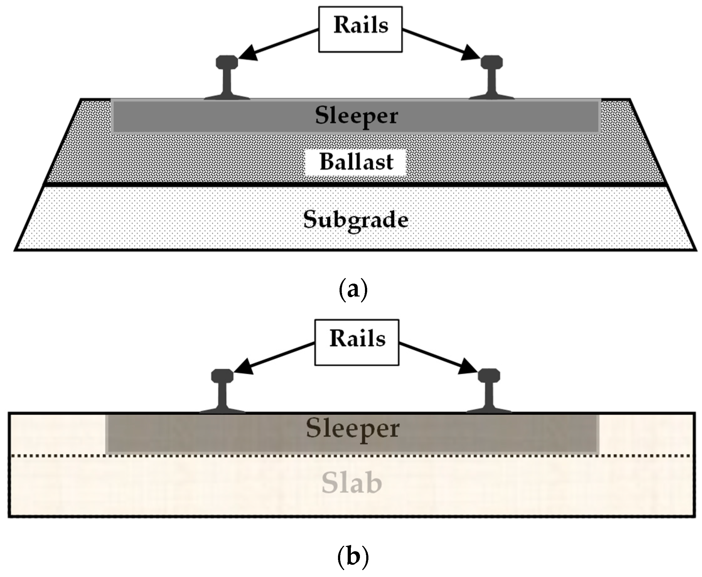
1.1. Type of Railway Sections: Ballasted and Ballastless

Traditional ballasted railway tracks (Figure 1a) consist of rails that are attached to sleepers, which in turn are supported by a layer of crushed stones (ballast) [17]. The ballast provides the elasticity that is needed to bear train loads. Subgrade and ballast are often separated by a bituminous or granular layer, the blanket (cf. [18]).

The other types of railway tracks are ballastless railway tracks (cf. Figure 1b; cf. [17,19,20,21]). The ballast is replaced with an upper layer consisting of cement concrete slabs, and a second layer, i.e., the hydraulically bonded layer (HBL; [17,21]).

The main differences between the two aforementioned types of railway tracks are [17,20]:

• Initial/capital costs (ballastless tracks are more expensive than ballasted ones; cf. [17,20]).
• Maintenance costs (ballastless tracks are cheaper than ballasted ones, especially in the long–term period; cf. [20]).
• Noise (ballastless tracks are noisier than ballasted ones; i.e., 2–4 dB (A) at 100–260 km/h; cf. [17]).
• Vibration (if softer rail fasteners are used, ballastless tracks can allow producing lesser ground–borne vibrations that are lower than for the ballasted ones, e.g., about 3 dB lower at frequencies lower than 64 Hz; cf. [22]).
• Stability (ballastless tracks provide higher longitudinal and lateral stability than the ballasted ones [20]).
• Ballastless tracks should not be used in areas prone to earthquakes or with softer soils (cf. [20]).
• When used in HSRs, ballasted tracks are open to the risk of flying ballast (i.e., trains travelling at high speeds can cause an aerodynamic force that displaces one or more ballast particles from the track. These particles can damage locomotives, railcars, and tracks, and can injure workers near tracks). This is a safety as well as an economic concern; cf. [20].
• Service life (ballastless tracks are more prone to fatigue failure than ballasted ones, especially when being used as HCR; cf. [23]. This could have consequences in terms of life cycle analyses).
• Environmental impact (for low service lives, e.g., lower than 60 years, ballasted tracks have lower environmental impacts. Note that the environmental impact of ballastless tracks depends also on the production of the steel for the track slab (cf. [23])).

Table 1. Strengths and weaknesses of ballasted and ballastless railway tracks.

Type	Ballasted
Strengths	More reliable (used for 150 years). Lower construction costs. Good drainage properties. Higher elasticity. Higher noise absorption levels. Simpler maintenance (e.g., components replacement, and geometry correction). Good subgrade settlements resistance and good movements compensation.
Weaknesses	Relatively short lifetime (20–30 years). High maintenance requirements. Heavier and have a higher structural height (not recommended on bridges and in tunnels). Not recommended for high speeds (proper design or proper improvements can reduce this problem). Lower lateral and longitudinal resistance (can cause “floating” track at high speeds, especially in curves). Ballast flight (also called ballast pick–up or churning) at high speeds. Ice flight in cold climate countries at high speeds. Not accessible to emergency vehicles.
Type	Ballastless
Strengths	More available. Long lifetime (up to 60 years). Very little to no maintenance requirements (maintenance costs about 20–30% lower, lower units of personnel on the track, lower number of accidents/injuries, and minimized or avoided vegetation control). Higher lateral and longitudinal resistance. No settlement problems (due to stable subsoil). Recommended for high speeds (higher longitudinal and lateral stability). Recommended on bridges and in tunnels. Accessible to emergency vehicles. Possibility to use electromagnetic wheel brakes (lower structural height and weight, which is good for bridges– and tunnel–related applications).
Weaknesses	Higher investment/construction costs (1.2–3 times higher). Poor subgrade settlements and movements compensation (this leads to structural damages). Very strict requirements for the subsoil and substructure. Complicated and cost–intensive maintenance (especially after a derailment). Noisier (absorbing materials on top of the track are needed to minimize the problem).

summarizes the main strengths and weaknesses of ballasted and ballastless railway tracks [7,24].

In [7], a decision–making model (based on Life Cycle Cost, LCC, Fuzzy logic, and Monte Carlo analysis) for the selection of appropriate solutions for HSR (among ballasted, ballastless or combined systems), as a function of several factors and requirements (technical, practical, or from national standards), was proposed.

1.2. High–Speed and High–Capacity Rail (HSR/HCR) Systems

The crucial year for the development of the HSR in the world was 1964, when the Tokaido Shinkansen was presented in Japan [25]. This was a line designed to connect Tokyo Central to Shin Osaka, with trains designed to operate at 210 km/h [25]. The first European HSR was presented in France in 1981 with an operating speed of 260 km/h [25]. In 1988, Italy and Germany presented the “Pendolino” and Inter–City Expres (ICE) HS trains, respectively [25]. From 1992 to 2009 [25], HS networks were developed in the U.S.A., Spain, Belgium, the U.K., South Korea, Taiwan, China, the Netherlands, and Turkey. In 2015 [25], 30,000 km of HS network were developed all over the world.

The common definition of High–Speed (HS) rail systems refers to technical criteria [25], i.e., operation speed of at least 250 km/h. However, a more comprehensive definition must take into account many technical aspects (e.g., infrastructure, rolling stock and operations) and strategic and cross–sector issues (e.g., human factors and financial, commercial, and managerial components) [25]. Importantly, the term “High–Speed” should not mask the performance as perceived by customers (e.g., travel time, frequency, comfort, and price; cf. [25]). From a technical point of view, HSR systems require:

• Special Trains: “train sets” are needed instead of conventional trains consisting of locomotives and cars. This depends on several reasons, such as the power–to–weight ratio, aerodynamics, reliability, and safety constraints.
• Special dedicated lines able to allow speeds above 200–220 km/h. This is a function of (2.1) Layout parameters, such as horizontal and vertical profiles, and the cant. (2.2) Transverse sections, track quality, catenary, and power supply. (2.3) Particular environmental conditions to ensure sustainability.
• Purpose–built signalling system line: above 200 km/h, in–cab signalling must be used instead of side signals, which may not always be observed in good time by the drivers.
• An HSR is a complex system that includes the state of the art in many different fields, such as infrastructure, stations, rolling stock, operations, maintenance strategy and corresponding facilities, financing, marketing, management, and legal issues and regulations [25].

The HS concept is strictly related to the concepts of capacity and sustainability [25,26,27]. In turn, capacity requires accessibility, complementarities, and a multimodal approach [25].

The French HSR network (Lignes à grande vitesse, LGV) was the first network developed in Europe in 1981. As of 2021, it comprises 2800 km and maximum speeds < 300 km/h [25,28]. As of 2022, the Spanish HSR network is 3762 km long (cf. also [29]). The new High–Speed Line Turin–Lyon is a part of the Mediterranean Core Network Corridor (Trans European Network–Transport, TEN–T, Core Corridor n.3, cf. [30]). This latter corridor will connect Spain with Eastern Europe. The central part of the HS line is the cross–border section that passes through Italy (i.e., using the Turin–Trieste route 65 km long). This line should be completed in 2029. The HS/AC lines in Italy [30,31] have been designed to allow for mixed train traffic including passenger and freight cars both for long and short distances (Turin–Lyon, Brenner, Turin–Milan, Milan–Verona, Verona–Padua–Venice, Milan–Genoa, Milan–Bologna, Bologna–Verona, Bologna–Florence, Florence–Rome, and Rome–Naples). The High Speed/High Capacity (HS/AC) project carried out in Italy by Italferr [30] refers to the Italian busiest network, 1250 km long (including the Turin–Venice line, and the Milan–Naples line), and to a partially new and partially under design/construction network 2200 km long (which includes cross–border links and connections to Southern Italy, i.e., from Naples to Bari, Reggio Calabria and Palermo) (

Table 2. Gradients.

Ref.	Details	Rail Slope for High–Speed Lines (Passenger Traffic Only) [mm/m; ‰]	Rail Slope for High–Capacity Lines (Freight Traffic Only) [mm/m; ‰]	Italy Rail Slope for High–Speed and High–Capacity Lines (Mixed Traffic) [mm/m; ‰]
[31,33]	International lines	35 (max value)	12.5 (max value)	–
[34]	AVAC Napoli–Bari	–	–	13 (max value)
[35]	AVAC Palermo–Catania–Messina	–	–	12–12.5
[36]	AV Battipaglia–Romagnano	–	12–18 (18 for difficult topography)	–
[37]	AVAC Bologna–Firenze	–	–	15 (max value)
[38]	AVAC Roma–Firenze	–	–	8 (max value; most of the line is straight)
[39]	AVAC Torino–Lyone	–	33 (old line)	12.5 (new line)
[40]	Roma–Pescara	–	≥25 (old line)	–
[41]	AVAC Treviglio–Brescia	–	–	15 (max value)
[42]	Potenza–oggia	–	–	28 (old line)
	Palermo–Trapani	–	5 (old line)	–
	AVAC Brennero lotto 1–Fortezza–Ponte Gardena	–	–	23 (old line) 12 (new line)
	Paola–Cosenza	–	12 (new line)	–
	AVAC Brennero tunnel	–	–	6.7 (Austrian side) 4 (Italian side)
[43]	Third Giovi pass	–	35 (max value)	–

). Doubts could emerge about several sections, where, despite the name (AVAC), speeds are lower than 300 km/h. In 2022, the HSR/AC is 1467 km long, while the entire railway network is 24,564 km long [32].

1.3. Railway Costs

The total cost of a railway system per km includes the cost of infrastructure, the cost of stations and substations (Traction substations), and the cost of rolling stock [44]:

$$C=C_{\mathit{INFR}}+C_{\mathit{STAT}}+C_{\mathit{ROLL}}$$

(1)

The design and the cost of an infrastructure depend on a number of factors, including the tonnage per day, the type of traffic, and axle loads.

For example, the train “Frecciarossa 1000”, which is mainly used in Italy, has an axle load of about 17 tons [45]. Freight–dedicated railways along TEN–T Corridors will be adapted according to European standards to allow trains up to 750 m long to operate and to support an axle load of up to 22.5 tonnes [46].

Infrastructure costs, C_INFR above (sometimes termed total investment cost, cf. [47]), include:

• The cost of design and planning. These costs are regulated by national standards (e.g., ministerial decree 17 June 2026 for Italy [48]). When construction works are higher than 25 million euros, they cannot be higher than 10% of the total cost of infrastructure.
• The costs of land acquisition and management (sometimes called ancillary costs, see Assessment of unit costs (standard prices) of rail projects [47]). They mainly depend on the type of land.
• The cost of the track (or permanent way, cf. [47], or superstructure). This includes the cost of rails, fastening systems, sleepers, ballast (crib, top, and bottom ballast, cf. [49]), and switches. The increase in axle load implies the increase in cost of many components, including rails, ballast, and subgrade, due to the use of better materials (e.g., modulus increase for subgrade) and/or different geometry (e.g., for rails and ballast, cf. [50]). The increase in construction costs depends on many factors because it basically derives from a design concept, namely having the same expected life of tracks and viaducts or accepting an appreciable increase in maintenance costs. Based on the proportionality between stresses and loads, a very approximate figure for the increase in terms of costs would be 30%. This estimate has intrinsic limitations because the deterioration depends on many factors, including [51]: (1) The type of failure (e.g., rail fatigue, rail surface defects, fatigue of other components, and track geometry deterioration). (2) The tonnage. The daily tonnage may vary, for example, from less than 10,000 t/day to more than 40,000 t/day and, for the sake of dimensioning and maintenance; it is derived in terms of equivalent tonnage. This latter, in turn, depends on speed, real load for daily passenger traffic, real load for daily freight traffic, maximum axle load and geometry of wheels. (3) The total load (static and dynamic). (4) The speed. (5) At least four supplementary factors, partly dependent on the type of failure. For the track, based on the above, and based on ORE D161 rp3 (Dynamic vehicle track interaction phenomena from the point of view of track maintenance), [51] points out that the increase in cost (maintenance) depends on axle load, track quality, and speed, and that the increase in axle load from 20 t to 22.5 t implies higher maintenance costs (+8–10%, the remaining factors being constant):

$$E=k·T^{\alpha }·P^{\beta }·V^{\gamma }$$

(2)

where E is the deterioration (e.g., since renewal or last maintenance operation, cf. [51]), T is the tonnage, P is the total axle load (static and dynamic), V is the speed, while k, α, β, and γ are constants. Note that, based on the type of phenomenon involved (i.e., rail fatigue), α ranges from 1 to 3 and beta from 3 to 3.5.

○

To this end, it is important to note that this is consistent with road pavement–related studies and, namely, with [52] expression of the equivalent axle load factor:

$$\mathit{EALF}={\left(\frac{{\epsilon }_x}{{\epsilon }_{18}}\right)}^4$$

(3)

○

with a coefficient f₂ = 4 in the Asphalt Institute formula

$$N_f=f_1{\left({\epsilon }_t\right)}^{-f_2}·{\left(E_1\right)}^{-f_3}$$

(4)

○

and, finally, with (3) AASHTO and Asphalt Institute equivalent axle load factors.

• The increase of cost for track and viaduct construction due to higher axle loads is herein taken into account through a factor (hereafter called “ACF”, high capacity factor, where high capacity here stands for open to freight traffic). Note that this pertains to the paradigm shift toward Lean, Agile, Resilience and Green (LARG) solutions [7], as the opposite of the AVAC (HS–HC) solutions.
• The cost of the platform (cf. [53]). This does not include the superstructure and it is usually termed building cost [44]. This cost depends on the length and type of (1) Viaducts and bridges. (2) Tunnels. (3) Earthworks. These latter do not include the cost of ballast, while including the cost of the soils (layers) below the ballast (e.g., sub–ballast, blanket, and subgrade (placed soil and natural ground). More specifically, they include tracking, roading, cleanfill sites, cut and fill operations, quarrying/mining and transport, and re–contouring [47].
• The cost of signalling, electrification, and telecommunication (cf. [44,47]).
• The cost of fencing and noise barriers.

Note that the REGIO Rail Unit Cost Tool [47] reports the unit costs for high–speed and conventional lines. Note also that, based REGIO [47] and on EU Council Directive 96/48/EC, the difference is as follows:

• High–speed lines are classified as newly built infrastructure that can be operated at a speed that is equal to or higher than 250 km/h or that results from an upgrade of a pre–existing line which can then be operated at speeds of at least 200 km/h.
• Conventional lines are classified as newly built infrastructure that can be operated at a speed lower than 250 km/h or an existing line that can be operated at a lower speed than 200 km/h.

Table 3. Examples of cost items for double track @high speed and conventional track (Millions of euros per kilometre).

	Double Track, High Speed
	Literature	Conventional	Model Variable
Design and planning	<10% [48]
Land acquisition			0.4
Rails	0.16 [53]	1.1–1.7 [47]	1
Fastening systems + Sleepers	0.22 [53]
Ballast	0.14 [53]
Switches	0.22 [53]
Viaducts and bridges	20–50 [54]		35
Tunnels	20–70 [54]		40
Earthworks	3.4 [47]; 1–4 [44]	0.9 [47]	2.3
Signalling	0.3–1 [44]; 0.5 [47]	0.3 [47]	1.3
Electrification	0.7–1.2 [44]; 0.6 [47]	0.6 [47]
Telecommunication	0.19 [47]	0.3 [47]
Fencing and noise barriers	0.8 [47]

,

Table 4. Cost items of the infrastructure cost.

Cost Item	Task	Amount
CSTUD	Feasibility study, preliminary study and project.	0.01–0.1 M€/km. 0.3–3% of the total investment
CLAND	Acquisition of land and rights, which depend on population density.	N.A.
CBUILD	Preparation of the ground, embankments, drainage, structures (walls, water ducts, bridges, tunnels, overpasses and underpasses), fences and noise–protection equipment, service access roads, interim financial charges, general expenses, and initial additional maintenance.	Single track *: 21–85 M€/km. Double track *: 51–140 M€/km.
CTRACK	Acquisition and installation of ballast, sleepers, rail fastening, rails, welds or fish–plates, laying, and initial additional maintenance.	0.2–0.6 M€/km for rail mass of 50–70 kg/m.
CELECT	Electrification of substations, catenary, lowering the floor in tunnels, raising overpasses, modification of signalling equipment along the track and in stations, and telecommunications equipment.	Single track *: 0.5–0.9 M€/km. Double track *: 0.7–1.2 M€/km.
CSIGN	Acquisition and installation of cables, automatic block system, spot repetition of signal (automatic train protection or advanced train protection), cab signal (automatic train control), the radio link between the dispatcher and the train, and level crossing with light and acoustic signals and automatic barriers.	Single track *: 0.3–0.5 M€/km. Double track *: 0.3–1.0 M€/km.

Notes. * Cost ranges for single and double tracks were derived by summing minimum and maximum values related to easy and average topography difficulty, tunnels, and bridges.

and

Table 5. Cost items of the operating cost.

Cost Item	Task	Amount
CTR	Powering the trains, which depends on the number of trains per kilometre (i.e., the product of runs and the total length of the line), of the unit cost of the power source (i.e., electricity or diesel, e.g., measured in €/kWh and €/litres, respectively), and of the unit consumption (measured in kWh/km for electric trains, and litre/km for diesel trains).	Electric regional train *: 0.2–0.9 €/km. Diesel train: 0.8–1.9 €/km.
CDEP	Depreciation of the rolling stock cost over a given period (usually 20 years).	Recent fleets: about 33% of the total cost of the service; Old fleets (≥20 years): 8–10% of the total cost of the service.
CMAN	Maintenance of the rolling stocks, which depends on fixed management costs (about 30–40% of total maintenance cost), variable costs for worn parts replacement (5–10%), fixed and variable costs related to the workshops (50–60%), and exterior and interior cleaning of rolling stock (0.05–0.1%).	e.g.: Local and suburban trains: 2.5 €/train–km for electric trains, and 3.5 €/train–km for diesel trains.
CSAL	Ground services (operating personnel or indirect personnel) and services on board the train (e.g., drivers, conductors and ticket inspectors). Ground personnel cost is independent of service, while onboard personnel cost depends on the operating time.	N.A.
CACC	Access to the service. This depends on the company that provides the service.	e.g.: Local and suburban trains: About 0.1–5.2 €/train–km.

Notes. * Range derived considering 1 train/km.

summarize examples of cost estimates.

In [44], a model for estimating railway–related investment and operating costs at a regional level is presented. In Italy, this model considers the railway–related cost as the combination of two main components (first/high–level analysis or bird’s eye view), i.e., investment costs (which include costs related to infrastructure, station and other fixed equipment, and rolling stock) and operating costs (which include traction, depreciation, maintenance, salaries, and access charges). In turn, the infrastructure investment cost (C_INFR) is considered as the sum of the following cost items (cf. Table 3): (1) Study costs (C_STUD); (2) Land costs (C_LAND); (3) Building costs (C_BUILD); (4) Trackage costs (C_TRACK); (5) Electrification costs (C_ELECT); (6) Signalling costs (C_SIGN). Further details are reported in the table below (Table 4 and Table 5; [44]). At the same time, the operating costs (C_OPE) are defined by [44] as the sum of different items, i.e.,: (1) Traction cost (C_TR); (2) Rolling stock depreciation cost (C_DEP); (3) Rolling stock maintenance cost (C_MAN); (4) Salary cost (C_SAL); (5) Access fees (C_ACC).

In [55], 166 HSR projects are analysed. These authors reported International Union of Railways (UIC) data (2005), which considered three main classes of costs for building HSR infrastructures: (1) Planning and land costs (5–10% of the total investment amount); (2) Infrastructure building costs (10–50% in lines with high complexity, e.g., where viaducts, bridges, or tunnels are needed); (3) Superstructure costs (5–10%). After construction, HSR infrastructure costs refer to (1) exploitation and maintenance, and (2) provision of transport services. Based on the data reported in [55], which refer to HSRs built in Austria, Belgium, France, Germany, Italy, Japan, Korea, Netherlands, Spain, and Taiwan, the average costs for the construction and maintenance of the infrastructures range between 24–48 M€/km, while the average costs related to the acquisition, operation and maintenance of a single HSR train range between 27 and 53 M€/train. The sum of these amounts can be assumed as an estimation of total cost, and is in the range 29–101 M€/km.

Ref. [56] reported a range of costs for infrastructure construction and rolling stock acquisition of 35–70 million USD/km (based on several international projects). Usually, capital costs are higher than operating and maintenance costs (often because of the high technical complexity of projects, or delays), and it is almost impossible to regain the operating and maintenance costs from the passengers (very densest traffic corridors, e.g., 20 million of passengers/year, or efficient marketing strategies, e.g., discounts that aim at filling unused seats, are needed to minimize the problem; cf. [56]). Consequently, authorities that want to build an HSR have to take into account the need for continuous and copious budget support for the debt certainly accumulated, and aiming to obtain a very high number of passengers per year (e.g., >40 million; cf. [56]) to have a chance of recovering at least the capital costs. In 2010, China had the best characteristics required for the success of the HSR technology, i.e., very high population density, rapidly growing disposable incomes, and a string of large cities (instead of city pairs). These characteristics are crucial for reducing costs and accelerating the recovery of investments.

Ref. [57] presented the results of a simulation that aimed to define all HSR costs based on [55]. In particular, the simulation considered a connection between two similar–sized cities consisting of a completely new single line 500 km long, without intermediate stops, with a service life of 40 years (5 years for planning, land acquisition, and construction, and 35 for operations), and a commercial speed of 250 km/h. Note that the authors stated that 40 years was the average useful life of a train in 2009. Another input assumption of the simulation has been a demand of 5 million passengers per year (during the operational period of 35 years), symmetrically distributed along the two cities, during the day and during the year, and with a growth rate of 5% until the 11th year and 3% for the remaining years. A train capacity of 330 seats has been selected considering the three commonly used train capacity classes, i.e., low–capacity trains (200–250 seats), medium–capacity trains (300–400 seats), and high–capacity trains (more than 500 seats). The train frequency (Ft; i.e., numbers of services per hour) was calculated considering the daily demand (qt), the effective occupation of the trains (qe; under the hypothesis of a load factor of 75%), and that trains operate 18 h per day. The train supply (i.e., the number of rolling stock needed at a given service year) was derived considering the aforementioned parameters qt, qe, and Ft, and the additional parameters τ (total travel time, which is equal to 4.5 h in the simulation) and a contingency factor (which takes into account possible delays, damages, etc.) of 1.5 (depending of the corridor, typical values are in the range 1.25–1.6). Based on the input parameters mentioned above, the HSR–related total cost (TC), which was expressed as the net present value of the sum of the infrastructure cost (IC) and rolling stock cost (RSC), was derived. In particular, IC (related to building, operating and maintaining tasks) was expressed as a function of the actual values of the average costs per km (for construction and maintenance, called c and m, respectively), the line length, a construction surcharge of 10%, the service life, and a discount rate (i) of 5%. RSC was considered as the sum of the train–related acquisition, operation, and maintenance costs. Based on the above, the authors provided three values of the total cost, TC, related to three scenarios, i.e., best (lowest infrastructure–related costs, cheapest trains, lowest train operation and maintenance costs), medium, and worst. These values are about 8, 13, and 24 billion euros (B€) for the best, the medium, and the worst scenario, respectively (i.e., about 15, 26, and 48 M€/km). In addition, the authors provided the estimation of the total costs for alternative assumptions and for the three scenarios mentioned above: (1) For an initial demand ranging from 2.5 to 20 million passengers, TC is included in the ranges 6–18, 11–26, and 21–40 B€ (note that lower costs refer to lower numbers of passengers); (2) for train capacity ranging from 330 to 500 seats, TC results in the ranges 7.6–7.7, 12.9–13, and 23.7–23.8 B€ (note that lower costs refer to a higher number of seats); (3) for commercial speeds in the range 200–300 km/h, TCs are 7.3–8.4, 12.4–13.9, and 23–25 B€ (note that lower costs refer to high speeds); and (4) for line lengths between 250 and 650 km, TCs are 4.1–9.9, 6.8–16.7, and 12.2–30.7 B€ (note that lower costs refer to low line lengths).

Ref. [58] suggested that market prices should be used instead of resource costs to present the economic results of HSR investments, and user income (or some proxy, e.g., journey purpose) should be segmented to define HSR–related impacts on users. Based on data from U.K. HSR services and market prices analyses, gross benefits can be mainly attributed to time–saving (about 50% of the total gross benefits), revenue (about 30%), reductions in rail overcrowding (about 10%), and other environmental and economic benefits. In Europe, HSR demand in 2013 [14] was subtracted from the air (about 30%), from classic rail (about 30%), and from roads (about 15%), while 25% was generated (high levels of generation are obtained in developing countries, where air market is not yet mature or public transport is predominant). High population densities, high land values, and unfavourable topography dramatically affect the capital costs (e.g., from below 10 M€/km in China, to over 100 M€/km in the U.K.), which mainly depend on operating speed (e.g., in China, capital costs double for operating speed of 350 km/h in comparison to a speed of 250 km/h). In 2013, very different HSR demands were observed all over the world (including 4 million passengers per year in Spain versus 200 million in Japan), and gravity model formulations can be used to define the main factors that affect this demand (e.g., fare levels, cities, stations, and population distribution, incomes, changes in economic structures, and socio–cultural barriers). Commonly, intermodal completion between HSR and air, road, and sea markets is observed worldwide, unlike in Italy where the intra–modal competition between the companies Trenitalia and Italo–NTV led to a fare reduction (30%) and increases in service and demand (45%, and 30%, respectively). Finally, [14] suggested the use of a step–by–step approach for the HSR investments and provided the following guidelines: (1) Use the level of passenger demand as a key metric. (2) Use gravity model formulations to carry out high–level strategic forecasts in advance, before carrying out detailed modelling estimations. (3) Consider, at a network level, incremental HSR investments. (4) Identify the best lines, and then plan the network evolution. (5) Prefer line extensions instead of new lines (if possible). UIC (2015) [25] reported the following costs for HSRs: (1) construction: 15–40 M€/km; (2) annual maintenance: 90,000 €/km; (3) HS train of 350 places: 30–35 M€; (4) HS train maintenance: 1 M€/year. [59] analysed the impact of axle loads on rail infrastructure (track substructure and track superstructure) maintenance costs. Results show that maintenance costs increase when the tonnage per axle increases, and this can affect track access charges that in turn affect the marginal costs in EU member states (i.e., charges of low average tonnage per axle trains subsidise those of high average tonnage per axle ones).

Based on [60], the following conclusions can be drawn:

• Lower slope–increased length of the track–higher construction cost and maintenance cost.
• Freight traffic–increased gauge clearance–increased construction and maintenance cost.
• Increased load–increased cost of the platform (rails sleepers and ballast and blanket and subgrade).
• Increased load–increased rail maintenance cost.

It is important to underline that besides the economic costs (defined above), there are other costs, usually called “external costs”. [55] reported example of “external costs” (e.g., land take, barrier effects, visual intrusion, noise, air pollution):

(1)

CO₂ emission related to the transport of 100 passengers/km of 4, 14, and 17 tonnes for HSRs, private cars and aeroplanes, respectively.

(2)

Noise of an HSR train is 80–90 dB (A) at different speeds. It was estimated that, if no barriers are used and when a train travels at a speed of 280 km/h, a corridor of 150 m is needed to decrease the noise level at an acceptable value of 55 dB (A).

UIC reported a virtuous project carried out in California [25]. The construction of the new HSR was accompanied by a carbon offset consisting in planting 4600 trees and donating 20 million US dollars for the replacement of old school buses. These carbon correction measures will make the GHG pollution of HSRs 43 and 57 times lesser than those of cars and aeroplanes, respectively. Based on the advantages offered by the HS systems (e.g., high speed, fully electrified transport chain, CO₂ saving), it seems reasonable to imagine shifting freight transport from road to rail [61] or from airline to rail [62] (especially for low–density high–value goods). [61] estimated that HS freight can enable reducing CO₂ emissions (e.g., 80%) in comparison with road–based lorry transport, although it is more expensive (e.g., 70%). [11] reported that shifting from airline to rail can be a good way to respond to the increasing needs related to mobile shopping and e–commerce. These authors identified several advantages for air transport, HSR, customers, and society (e.g., reduction of costs, pollution, and congestion; improvements in terms of demand, quality of service, and safety). Finally, they stated that this result can be obtained but that great efforts, in terms of cooperation among different infrastructure authorities, the preventive maintenance (e.g., sensor–based) instead of the breakdown one, investments in proper infrastructures (e.g., terminals), are needed.

2. Objectives and Scopes

At the planning stage, the estimation of railway costs is crucial to better select the best solution. This applies also to the well–known problem of selecting the best solutions for South Italy and pertains to the main objectives of the aforementioned Italian PNRR/NRRP, National centre for sustainable mobility–SP4.

Despite this, in view of the foregoing, there is a lack of sustainable models and tools to use for cost estimates.

Based on the above, the main objectives of the study presented in this paper have been confined to the setup of a model for the estimation of HSR and HSR/HCR infrastructure cost. The model was calibrated and validated. Theoretical considerations and data were derived from Italian (both HSR and HSR/HCR), Spanish, and French HSR projects.

The following tasks were carried out:

• Task 1: Analysis of the literature (see Section 1).
• Task 2: Set up of the model (cf. Equation (10), see Section 3).
• Task 3: Calibration of the model (see Section 4.1).

  ○

  Sub–Task 3.1: Speed factor (herein called “SF”, based on [54]).

  ○

  Sub–Task 3.2: National Factor (herein called “NF”) and High–Capacity factor (herein called “ACF”).

• Task 4: Validation (see Section 4.2).

The remaining parts of the paper refer to the definition of the aforementioned model (cf. Section 3) and the validation and application of this model (cf. Section 4). Finally, the main conclusions (cf. Section 5) and references are reported.

3. Modelling

In this section, the model herein set up is presented. Based on the above, and considering Equation (1), the following main components are considered (Cf.

Table 6. Railway type and related factors.

Railway Type	Tentative Values
	ACF	SF
A = High–speed and high–capacity (HSHT = AVAC)	>1	=1
B = High speed (without freight traffic, HS = AV)	=1	=1
C = Conventional (V < 250 km/h, mixed traffic; AC)	>1	<1
D = Low–speed and low–capacity	=1	<1

and Figure 2):

$$\begin{array}{c}{C}_{INFR}={\displaystyle \sum _{j=1}^7}{C}_j=C_1+C_2+C_3+C_4+C_5+C_6+C_7=\\ =C_{DES}+C_{LAND}+C_{TUN}+C_{VIAD}+C_{EARTH}+C_{SUP}+C_{SET}\end{array}$$

(5)

where C_INFR is the estimated infrastructure cost [Millions of euros per kilometre, M€/km], while C_DES, C_LAND, C_TUN, C_VIAD, C_EARTH, C_SUP, and C_SET are, respectively, the cost items related to project design, land acquisition, construction of tunnels and viaducts, earthworks, and construction of the superstructure (i.e., ballast or ballastless section described above), and train–station connection and train powering (i.e., signalling, electrification, and telecommunication) [Millions of euros per kilometre, M€/km]. SF, ACF and NF are three factors introduced by the authors of the current study, herein called Speed Factor (SF, where SF is supposed to increase with the speed), high–capacity factor (ACF, where AC derives from the Italian “Alta Capacità”, and is supposed to increase with tonnage), and national factor (NF).

Note that the speed factor is here modelled as a function of the speed of the train (e.g., for high–speed railway S must be greater than or equal to 250 km/h) by considering 300 km/h as reference speed, and a parameter δ to calculate. Note that this factor was introduced to include the effect of train speed on infrastructure costs, based on the data reported in [54].

$$SF={\left(\frac{S}{300}\right)}^{\frac{1}{\delta }}$$

(6)

For C_DES, let us suppose that:

$$C_{DES}=K_{DES}·{\displaystyle \sum _{j=2}^7}{C}_j, \mathrm{with} K_{DES}\le 0.1.$$

(7)

where

$${\displaystyle \sum _{j=2}^7}{C}_j=C_{LAND}+C_{VIAD}+C_{TUN}+C_{EARTH}+C_{SUP}+C_{SET}$$

(8)

In turn, each j–th component above can be decomposed into multiple ji components:

$$C_j=C_{j1}+C_{j2}+C_{j3}+\dots +C_{jn}$$

(9)

With the aim of explaining the variation of infrastructure costs in different countries and contexts (speed, type of rolling stock(e.g., passenger or freight)), all the coefficients analysed above have been grouped into three main classes. In particular, the cost (per kilometre) of these components is herein affected by train speed (SF_ij), tonnage and loads (ACF_ij), and national factors (NF_ij), where

$$C_{INF}=\sum _j\sum _i{C}_{ij}^{\ast }·S{F}_{ij}·AC{F}_{ij}·N{F}_{ij}$$

(10)

In more detail: (1) SF (speed factor) is based on data analysis and builds on the fact that higher speeds imply higher forces and requirements. (2) ACF (high capacity factor, where capacity here means open to freight traffic) takes into account that the expected life of a rail track depends on axle load and tonnage, cf. Equation (2)). (3) NF (national factor) takes into account that each country has its own characteristics (economy, labour system, taxes, cost structures, and differences in competitive situations) and that this could affect costs. Furthermore, it is here supposed that:

$$\begin{array}{l}{C}_2=C_{LAND}=\\ =C_{\mathit{LAND}\_\mathit{ACQUISITION}}+C_{\mathit{LAND}\_\mathit{ANCILLARY}}\cong 0.4M€/km\end{array}$$

(11)

$$\begin{array}{l}{C}_3+C_4+C_5=C_{\mathit{PLATFORM}}=\\ =C_{\mathit{TUN}}+C_{VIAD}+C_{\mathit{EARTH}}=\%T·C_{u,T}+\%V·C_{u,V}+\%E·C_{u,E}\end{array}$$

(12)

$$\begin{array}{l}{C}_6=C_{\mathit{SUP}}=\\ =C_{\mathit{RAILS}}+C_{\mathit{SLEEPERS}}+C_{\mathit{FASTENERS}}+C_{\mathit{BALLAST}}+C_{\mathit{SWITCHES}}+C_{\mathit{EXPANDERS}}\end{array}$$

(13)

$$\begin{array}{l}{C}_7=C_{\mathit{SET}}=\\ =C_{\mathit{SIGNALLING}}+C_{\mathit{ELECTRIFICATION}}+C_{\mathit{TELECOMMUNICATION}}\end{array}$$

(14)

where %V is the ratio between the total bridges and viaducts length and the total section length [dimensionless, %], C_uV is the unit cost of a double track bridge/viaducts [M€/km], %T is the ratio between the total tunnels length and the total section length [dimensionless, %], C_uT is the unit cost of a double track tunnel [M€/km], %E is the ratio between the total earthworks length and the total section length [dimensionless, %; note that this percentage is derived as 1 − %T − %V], C_uE is the unit cost for medium/complex earthworks (i.e., cutting slopes and embankments with heights equal or greater than 0.5 m) for a double track [M€/km], C_SUP is the unit cost for the superstructure (i.e., rails, sleepers, fasteners, switchers, expanders, ballast/ballastless layer, and sub ballast/ballastless layer, which includes earthworks with heights lower than 0.5 m), and C_SET is the unit cost for the signalling (S), electrification (E), and telecommunication (T) of the line. Note that the factors above (NF_ij, SF_ij, and ACF_ij) can be merged at different levels. Consequently, the following simplified equation can be proposed:

$$\begin{array}{l}{C}_{INFR}={\displaystyle \sum _{j=1}^7}{C}_j·N{F}_j·S{F}_j·AC{F}_j=\\ =C_{DES}+C_{LAND}+(SF·NF)·\left[{\displaystyle \sum _{j=4}^7}{C}_j·ACF+C_{TUN}\right]\end{array}$$

(15)

Importantly, an additional factor must be here introduced because of the effect of freight trains on the total length of the track due to different slopes. Indeed, HSHC and HC lines have gradients usually lower than 12.5‰, while HS lines have gradients usually lower than 35‰ (cf. Table 2). This implies that the length of HC lines is higher than the one of the only passenger lines HS:

$$L_{HC}=K_{HC}·L_{HS}, \mathrm{where} K_{HC}\cong 2.8.$$

(16)

This tentative value of K_HC was derived based on 35‰ and 12.5‰, where the rationale behind K_HC is that freight trains need gradients “as gentle as possible”, and this could imply longer tracks.

Note that while ACF mainly refers to tonnage and load effects, K_HC mainly refers to traction–related issues. It follows that the cost of a given railway infrastructure (RC, M€) connecting two stations is:

$$RC=C_{INF}·L$$

(17)

where L is affected by freight trains. The equations above provide the researchers with a tool to analyse or predict costs. Anyhow, at a planning level, these tools include many pieces of information and there is a need for simplification.

From a macroscopic standpoint, let us consider what follows:

$$\sum _j\sum _i{C}_{ij}·N{F}_{ij}·S{F}_{ij}·AC{F}_{ij}=\left[\sum _j\sum _i{C}_{ij}\right]·NF·SF·ACF$$

(18)

To a first approximation, let us consider some–country comparisons and four main types of railway tracks as per Table 6.

Under the aforementioned assumptions, it follows that:

$$C_A=\sum _j\sum _i{C}_{A,ij}·N{F}_{A,ij}·S{F}_{A,ij}·AC{F}_{A,ij}$$

(19)

$$C_B=\sum _j\sum _i{C}_{B,ij}·N{F}_{B,ij}·S{F}_{B,ij}·AC{F}_{B,ij}$$

(20)

Subsequently, making the appropriate simplifications, the following relationships can be derived:

$$C_A=C_B·\frac{N{F}_A}{N{F}_B}·\frac{S{F}_A}{S{F}_B}·\frac{AC{F}_A}{AC{F}_B}=C_B·1·1·\frac{AC{F}_A}{1}=C_B·AC{F}_A$$

(21)

$$C_A=C_C·\frac{N{F}_A}{N{F}_C}·\frac{S{F}_A}{S{F}_C}·\frac{AC{F}_A}{AC{F}_C}=C_C·1·\frac{1}{S{F}_C}·1=\frac{C_C}{S{F}_C}$$

(22)

$$C_A=C_D·\frac{N{F}_A}{N{F}_D}·\frac{S{F}_A}{S{F}_D}·\frac{AC{F}_A}{AC{F}_D}=C_D·1·\frac{1}{S{F}_D}·\frac{AC{F}_A}{1}=C_D·\frac{AC{F}_A}{S{F}_D}$$

(23)

Importantly, when comparing data that refer to different countries, a national factor is supposed to be in place. For example, when comparing the Italian high–speed, IT (which actually is a high–speed and high–capacity railway), and the Spanish high–speed, SP, the following applies:

$$C_A\left(IT\right)=C_B\left(SP\right)·\mathit{Capacity}\_\mathit{factor}·\frac{\mathit{IT}\_\mathit{National}\_\mathit{Factor}}{\mathit{SP}\_\mathit{National}\_\mathit{Factor}}$$

(24)

Figure 2 summarizes both the hierarchical framework of costs and how the four classes of coefficients (i.e., high capacity, speed, national, and freight–related factors, ACF, SF, NF, K; Equations (16) and (18)) apply at different levels of detail.

4. Results and Discussions

Once the model was set up, it was calibrated by considering nineteen cases (six International cases + five Spanish cases + eight Italian cases, cf.

Table 7. The data set used in this study in model calibration and validation.

Ref.	Case Study	Use	Number of Cases
[54]	Baumgartner 2000 (M€/km for double tracks with speeds equal to 100 and 300 km/h for easy, average, and difficult topographies, for double track tunnels and easy and complex bridges).	CALIBRATION. Estimation of the unit cost of tunnels and bridges, and the parameter δ.	6 International cases (SF based on Equation (3), ACF = NF = 1)
[29]	Spanish HS lines: Cordoba–Malaga; Madrid–Siviglia; Barcellona–Figueres (French border); Madrid–Galizia; Madrid–Valladolid.	CALIBRATION. Estimation of the National Factor (NF) for five Spanish lines.	5 Spanish cases (SF based on Equation (3), ACF = NF = 1)
[34,35,36,37,39,41,63,64]	Italian HSHC lines: Battipaglia–Romagnano (1st batch); Brescia–Verona; Napoli–Bari; Palermo–Catania–Messina; Torino–Lione (Italian side); Treviglio–Brescia; Milano–Bologna; Bologna–Firenze.	CALIBRATION. Estimation of the National Factor (NF) and High–Capacity Factor (ACF) for Italy.	8 Italian cases (SF based on Equation (3))
[29,65,66,67,68,69,70]	Italian HSHC lines: Roma–Napoli; Torino–Milano; Verona–Vicenza; Verona–Padova (different sections). Spanish HS lines: Madrid–Toledo; Antequera–Granada; Almería–Murcia; Valladolid–Venta de Baños–Palencia–León. French HS line: Figueres–Perpiñan	VALIDATION. By using the NFs and the ACF mentioned above, the model (Equation (10)) was validated using four Italian lines, four Spanish lines, and one French line.	4 Italian cases + 4 Spanish cases + 1 French case = 9 cases (SF based on Equation (3))

) and it was validated considering nine cases (four Italian cases + four Spanish cases + one French case, cf. Table 7).

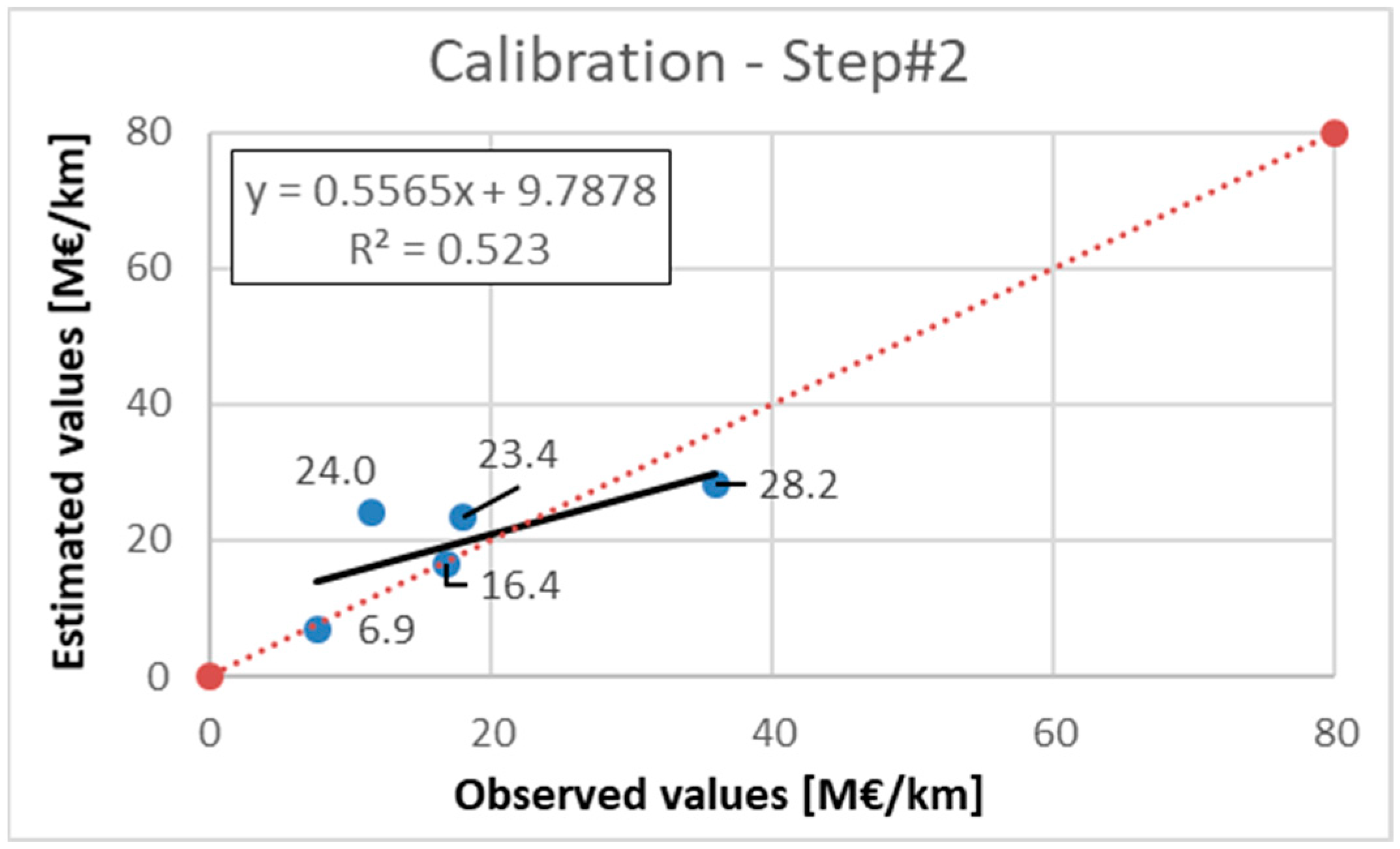
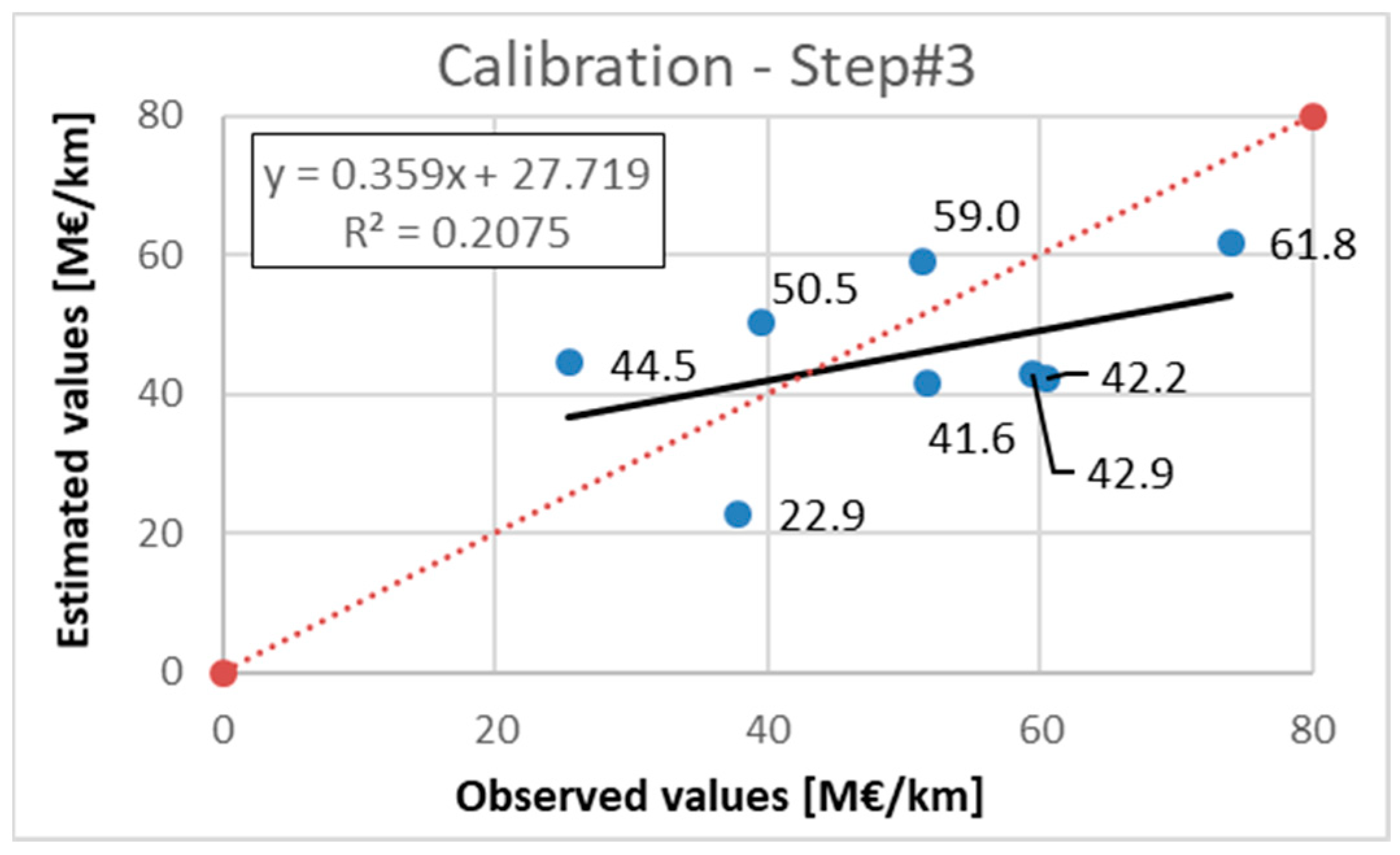
4.1. Model Calibration

For calibration, based on [54] and on Equation (18), the parameter δ and the following average unit costs were derived (Step #1 of the calibration):

• δ = 1.69;
• Tunnels: Cu_T = 45.58 M€/km;
• Viaducts: Cu_V = 40.46 M€/km;
• Earthworks (>0.5m): Cu_E = 2.13 M€/km;
• Superstructure: Cu_STR = 1.00 M€/km;
• Signalling (S), electrification (E), and telecommunication (T):
  Cu_SET = 1.29 M€/km;
• Land acquisition and ancillary = C_LAND = 0.40 M€/km.

Figure 3 illustrates the corresponding scatter plot where the x–axis reports the data gathered from the literature (cf. Table 7), while the y–axis reports the corresponding estimates (Equation (18)).

By referring to Step #2 of calibration, based on five HS Spanish projects, the following product was obtained: NF·ACF = 1.22 (where ACF = 1). Figure 4 illustrates the resulting scatterplot.

During Step #3 of the calibration, based on eight Italian HSHC projects, the product NF·ACF = 4.94 was obtained. Figure 5 illustrates the corresponding scatterplot.

4.2. Model Validation

Finally, for validation, nine case studies were considered. Figure 6a illustrates that two cases out of nine cases are quite far from the equality line. At the same time, Figure 6b shows the validation of the proposed model based on seven case studies (i.e., Figure 6a without the two aforementioned cases far from the equality line). In more detail, the two case studies deleted in Figure 6b are the line Roma–Napoli (observed value = 27.7 M€/km, estimated value = 62.8 M€/km) and different sections in the line Verona–Padova (observed value = 18.4 M€/km, estimated value = 52.5 M€/km).

Note that the validation carried out with seven case studies results in a higher determination coefficient. This calls for further investigation.

By way of example, possible applications of the proposed model include:

• Collecting the following inputs: cost of the land acquisition (C_LAND; or use Equation (11)), cost of the platform (C_PLATFORM; or costs of Equation (12) or % and unit costs of Equation (12)), train speed (S), railway type (e.g., single or double line), train/axle loads, cost of the superstructure (C_SUP; or all the costs of Equation (13) or estimate them based on similar project in the same nation), and cost of the signalling, electrification and telecommunication (C_SET; or all the costs of Equation (14) or estimate them based on similar project in the same nation).
• Estimating the following parameters: national factor (NF) and high–capacity factor (ACF) based on similar projects and Table 6, and speed–related factor (δ) based on similar projects.
• Deriving the following factor/parameter: speed factor (SF; Equation (6)), and cost of the infrastructure design (C_DES; Equation (8)).
• Estimating the infrastructure cost using the proposed model (Equation (15)), for the same context.
• Using the values (factors and parameters) herein derived to perform tentative estimates.

5. Discussions and Conclusions

High–speed railways (HSRs) are crucial for the social and economic development of regions and nations. Their design, construction, and maintenance should comply with many requirements, including the environment–, finance–, and policy–related ones. Based on the above, the main objectives of the study presented in this paper have been confined to the definition of a model for the estimation of HSR and HSR/HCR infrastructure cost and economic sustainability. Theoretical considerations and data derived from Italian (both HSR and HSR/HCR), Spanish and French HSR projects were used to set up and validate the proposed model. Based on the results, the following conclusions can be drawn:

• Under given conditions, it is possible to explain, through a national factor, why Italian HSR/HCR project costs are sometimes among the highest ones (based on the data set used in this study the average infrastructure cost for Italy is about 48 M€, while for Spain and France is about 17.5 M€). Importantly, apart from modelling, this could depend also on environmental factors (e.g., noise barriers) and mitigation strategies (e.g., funds for schools).
• Despite the high variability of infrastructure costs (mainly observed for the Italian projects), the proposed model allowed for obtaining high accuracy (R–square value = 0.98) in the estimation of the observed values.
• It is possible to explain part of the variance of results based on the following factors: (i) Speed of the line (Speed factor, SF); (ii) National factor, NF; (iii) Type of traffic and possibility of using the line for freight trains (K).
• At the same time, analyses demonstrate that the ACF, pertaining to tonnage, does not have an appreciable impact on the cost per kilometre. In contrast, freight trains impact track geometry (e.g., gradients) and the overall cost needed to link two destinations.
• Importantly, it is envisaged that the NF could be related to many elements, including mitigation actions (e.g., noise barriers and other funds addressing the improvement of conditions of life for the areas where the railway passes).
• For economic sustainability, it is envisaged that the transition towards railways that are high speed and also high capacity (in the sense specified above) implies higher expenses because of the high–capacity factor (ACF) and because of the longer track factor (K). Results and analyses demonstrate that while ACF is quite uncertain (due to the fact that many variables could mask its effect and the design is not LCC–based), K is definitely greater than 1. Furthermore, it is noteworthy to point out that lower gradients (freight trains) could imply higher percentages of viaducts and tunnels, having, in the end, consequences on ACF itself.
• Authors are aware of the limitations of the study (e.g., related to several low R–square values in calibration), because of the uncertainties in the information gathered and because many supplementary variables could be considered.

Future research will address a wider spectrum of case studies in the pursuit of performing further in–depth investigations and modelling.

References

1. Chang, Y.; Yang, Y.; Dong, S. Comprehensive Sustainability Evaluation of High–Speed Railway (HSR) Construction Projects Based on Unascertained Measure and Analytic Hierarchy Process. Sustainability 2018, 10, 408. [Google Scholar] [CrossRef] [Green Version]
2. Gherghina, Ş.C.; Onofrei, M.; Vintilă, G.; Armeanu, D.Ş. Empirical Evidence from EU–28 Countries on Resilient Transport Infrastructure Systems and Sustainable Economic Growth. Sustainability 2018, 10, 2900. [Google Scholar] [CrossRef] [Green Version]
3. Rungskunroch, P.; Yang, Y.; Kaewunruen, S. Does High–Speed Rail Influence Urban Dynamics and Land Pricing? Sustainability 2020, 12, 3012. [Google Scholar] [CrossRef] [Green Version]
4. Liu, X.; Schraven, D.; de Bruijne, M.; de Jong, M.; Hertogh, M. Navigating Transitions for Sustainable Infrastructures–The Case of a New High–Speed Railway Station in Jingmen, China. Sustainability 2019, 11, 4197. [Google Scholar] [CrossRef] [Green Version]
5. Økland, A.; Olsson, N.O.E.; Venstad, M. Sustainability in Railway Investments, a Study of Early–Phase Analyses and Perceptions. Sustainability 2021, 13, 790. [Google Scholar] [CrossRef]
6. European Commission. 96/48/EC Council Directive of 23 July 1996 on the Interoperability of the Trans–European High–Speed Rail System. Off. J. Eur. Union 1996, 235, 6–24. [Google Scholar]
7. Russo, F. Which High–Speed Rail? LARG Approach between Plan and Design. Futur. Transp. 2021, 1, 13. [Google Scholar] [CrossRef]
8. Russo, F. Alta Velocità al Sud: Linee Ferroviarie Adattate o Costruite? Available online: https://perfondazione.eu/alta–velocita–al–sud–linee–ferroviarie–adattate–o–costruite/ (accessed on 15 September 2022).
9. Pallavera, M. Linee AV/AC, le Ferrovie di Nuova Generazione. Available online: https://ilmegliodiinternet.it/cose–ferrovia–avac/ (accessed on 15 September 2022).
10. Connor, P. High Speed Railway Capacity: Understanding the Factors Affecting Capacity Limits for a High Speed Railway. In Proceedings of the International Conference on High Speed Rail, Birmingham, UK, 8–10 December 2014. [Google Scholar]
11. Doll, C.; Köhler, J.; Schade, W.; Simon, M.; Hasselt, E.v.; Vanelslander, T.; Sieber, N. European Freight Scenarios and Impacts. Summary Report 2: European Rail Freight Corridors for Europe—Storyline and Responsibilities; Fraunhofer: Karlsruhe, Germany, 2018. [Google Scholar]
12. IL Mezzogiorno in Movimento. Proposte e Progetti Verso IL Next Generation EU—Quaderno N.1/2021. Available online: www.sipotra.it/wp–content/uploads/2021/01/il–mezzogiorno–in–movimento.–proposte–e–progetti–verso–il–next–generation–eu–quaderno–n.–1–2021.pdf (accessed on 16 September 2022).
13. Merenda, M.; Praticò, F.G.; Fedele, R.; Carotenuto, R.; Corte, F.G. Della A Real–Time Decision Platform for the Management of Structures and Infrastructures. Electronics 2019, 8, 1180. [Google Scholar] [CrossRef] [Green Version]
14. Raczyński, J. Technical Parameters of High Speed Lines as the Determinant for Selection of Rolling Stock. In MATEC Web of Conferences; EDP Sciences: Les Ulis, France, 2018; Volume 180. [Google Scholar]
15. Herics, O.; Obermayr, T.; Puricella, P.; T’Joen, L.; Bode, M.; Böckem, D.; Fara, G.; Klis–Lemieszonek, A.; Odins, N.; Smid, M.; et al. A European High–Speed Rail Network: Not a Reality but an Ineffective Patchwork; European Union: Luxembourg, 2018. [Google Scholar]
16. Kaewunruen, S.; Sresakoolchai, J.; Peng, J. Life Cycle Cost, Energy and Carbon Assessments of Beijing–Shanghai High–Speed Railway. Sustainability 2020, 12, 206. [Google Scholar] [CrossRef] [Green Version]
17. Zhang, X.; Jeong, H.; Thompson, D.; Squicciarini, G. The Noise Radiated by Ballasted and Slab Tracks. Appl. Acoust. 2019, 151, 193–205. [Google Scholar] [CrossRef]
18. Pratico, F.G.; Moro, A.; Ammendola, R. Modeling HMA Bulk Specific Gravities: A Theoretical and Experimental Investigation. Int. J. Pavement Res. Technol. 2009, 2, 115–122. [Google Scholar] [CrossRef]
19. Schilder, R.; Diederich, D. Installation Quality of Slab Track—A Decisive Factor for Maintenance. RTR Spec. 2007. Available online: https://www.yumpu.com/en/document/view/25757280/installation-quality-of-slab-track-a-a-decisive-factor-for-maintenance (accessed on 16 September 2022).
20. Deng, J.; Liu, X.; Jing, G.; Bian, Z. Probabilistic Risk Analysis of Flying Ballast Hazard on High–Speed Rail Lines. Transp. Res. Part C Emerg. Technol. 2018, 93, 396–409. [Google Scholar] [CrossRef]
21. SÁRIK, V. Decision–Making Model for Track System of High–Speed Rail Lines: Ballasted Track, Ballastless Track or Both? Master’s Thesis, School of Architecture and Built Environment KTH Railway Group KTH Royal Institute of Technology, Stockholm, Sweden, 2018. [Google Scholar]
22. Ntotsios, E.; Thompson, D.J.; Hussein, M.F.M. A Comparison of Ground Vibration Due to Ballasted and Slab Tracks. Transp. Geotech. 2019, 21, 100256. [Google Scholar] [CrossRef]
23. Pons, J.J.; Villalba Sanchis, I.; Insa Franco, R.; Yepes, V. Life Cycle Assessment of a Railway Tracks Substructures: Comparison of Ballast and Ballastless Rail Tracks. Environ. Impact Assess. Rev. 2020, 85, 106444. [Google Scholar] [CrossRef]
24. Fedele, R.; Pratico, F.G.; Carotenuto, R.; Giuseppe Della Corte, F. Instrumented Infrastructures for Damage Detection and Management. In Proceedings of the 5th IEEE International Conference on Models and Technologies for Intelligent Transportation Systems (MT–ITS 2017), Naples, Italy, 26–28 June 2017; pp. 526–531. [Google Scholar]
25. Leboeuf, M. High Speed Rail Fast Track to Sustainable Mobility; International Union of Railways: Paris, France, 2018. [Google Scholar]
26. Praticò, F.G.; Vaiana, R. Improving Infrastructure Sustainability in Suburban and Urban Areas: Is Porous Asphalt the Right Answer? and How? In WIT Transactions on the Built Environment; WIT Press: Southampton, UK, 2012. [Google Scholar]
27. Wikipedia High–Speed Rail in the United States. Available online: https://en.wikipedia.org/wiki/High–speed_rail_in_the_United_States#First_attempts:_1960–1992 (accessed on 25 September 2022).
28. High Speed Rail Alliance TGV—Leader of the Integrated Network Approach. Available online: https://www.hsrail.org/tgv–leader–integrated–network–approach (accessed on 22 September 2022).
29. Adif Adif Alta Velocidad. Available online: https://www.adifaltavelocidad.es/ (accessed on 16 September 2022).
30. Italferr High Speed—High Capacity. Available online: www.italferr.it/content/italferr/en/proejct–studies/italy/alta–velocita–––alta–capacita.html (accessed on 22 September 2022).
31. Caratteristiche Tecniche delle Principali Linee Internazionali Ferroviarie (Allegato II). Available online: https://www.gazzettaufficiale.it/atto/serie_generale/caricaArticolo?art.progressivo=0&art.idArticolo=17&art.versione=1&art.codiceRedazionale=089G0159&art.dataPubblicazioneGazzetta=1989–04–24&art.idGruppo=0&art.idSottoArticolo1=10&art.idSottoArticolo=1&art (accessed on 22 September 2022).
32. Pagliara, F.; Mauriello, F.; Russo, L. A Regression Tree Approach for Investigating the Impact of High Speed Rail on Tourists’ Choices. Sustainability 2020, 12, 910. [Google Scholar] [CrossRef] [Green Version]
33. United Nations Economic Commission for Europe. Trans–European Railway High–Speed–Master Plan Study Phase 2—A General Background to Support Further Required Studies; United Nations Economic Commission for Europe: Geneva, Switzerland, 2021. [Google Scholar]
34. RFI AV/AC Napoli–Bari. Available online: https://www.napolibari.it/ (accessed on 22 September 2022).
35. RFI AV/AC Palermo—Catania—Messina. Available online: https://www.palermocataniamessina.it/content/fsipalermocataniamessina/it/il–progetto.html (accessed on 19 September 2022).
36. RFI. Nuova LineA av Salerno—Reggio Calabria Lotto 1A: Battipaglia—Romagnano (Dossier di Progetto); RFI: Paris, France, 2022. [Google Scholar]
37. Italferr Linea AV/AC Bologna–Firenze. Available online: https://www.italferr.it/content/italferr/it/progetti–e–studi/italia/alta–velocita–––alta–capacita/bologna–firenze.html (accessed on 25 September 2022).
38. Direttissima Roma–Firenze. Available online: https://www.italferr.it/content/italferr/it/progetti–e–studi/italia/alta–velocita–––alta–capacita/firenze–roma.html (accessed on 17 September 2022).
39. Asse Ferroviario Torino—Lione. Available online: https://presidenza.governo.it/osservatorio_torino_lione/ (accessed on 17 September 2022).
40. RFI. Raddoppio Linea Roma—Pescara (Lotti 1 e 2)—Dossier di Progetto; RFI: Paris, France, 2022. [Google Scholar]
41. Lombardi, F. AV/AC Treviglio Brescia. Available online: https://www.saipem.com/sites/default/files/2020-03/AV_Treviglio_Brescia_Cepav_Due.pdf (accessed on 17 September 2022).
42. Ministero delle Infrastrutture e della Mobilità Sostenibili. Contratto di Programma 2017–2021 Parte Investimenti Appendice N. 5 Alla Relazione Informativa—Schede Interventi CdP–I Agg. 2017–2021; Ministero delle Infrastrutture e della Mobilità Sostenibili: Rome, Italy, 2017.
43. Beria, P.; Grimaldi, R. An Early Evaluation of Italian High Speed Projects. Tema 2011, 4, 15–28. [Google Scholar]
44. Gattuso, D.; Restuccia, A. A Tool for Railway Transport Cost Evaluation. Procedia–Soc. Behav. Sci. 2014, 111, 549–558. [Google Scholar] [CrossRef] [Green Version]
45. Campione, D. IL Frecciarossa_1000. Available online: https://www.ferrovie.it/portale/articoli/782 (accessed on 28 September 2022).
46. Railwaypro Italy to Connect All Ports to the National Railway Network. Available online: https://www.railwaypro.com/wp/italy–to–connect–all–ports–to–the–national–railway–network/ (accessed on 28 September 2022).
47. PWC. Assessment of Unit Costs (Standard Prices) of Rail Projects (CAPital EXpenditure) REGIO Rail Unit Cost Tool Instructions; European Union: Luxembourg, 2018. [Google Scholar]
48. Ministero della Giustizia. Decreto Ministeriale 17 Giugno 2016—Approvazione delle Tabelle dei Corrispettivi Commisurati al Livello Qualitativo delle Prestazioni di Progettazione Adottato ai Sensi Dell’art. 24, Comma 8, Del Decreto Legislativo N. 50 Del 2016. Available online: https://www.bosettiegatti.eu/info/norme/statali/2016_dm_17_06_tariffe.htm (accessed on 24 September 2022).
49. Mpye, G.D.; Gräbe, P.J. The Effect of Increased Axle Loading on the Behavior of Heavily Overconsolidated Railway Foundation Materials. Transp. Geotech. 2021, 27, 100493. [Google Scholar] [CrossRef]
50. Lidmila, M.; Horníček, L.; Krejčiříková, H.; Tyc, P. Prerequisites for Increasing the Axle Load on Railway Tracks in the Czech Republic. Acta Polytech. 2008, 48. [Google Scholar] [CrossRef] [PubMed]
51. Esveld, C. Modern Railway Track; MRT–Productions: Zaltbommel, The Netherlands, 2001. [Google Scholar]
52. Deacon, J.A.; Fin, F.N.; Hudson, W.R.; Hindermann, W.L.; Warden, W.B.; Monismith, C.L. Load Equivalency in Flexible Pavements. Assoc. Asph. Paving Technol. Proc. 1969, 38, 465–494. [Google Scholar]
53. Andrés, A.; Mónica, G.; Gutiérrez, L. Costs and RAMS Methodologies (Superstructure). In Proceedings of the Dissemination Workshop, Paris, France, 10 June 2015. [Google Scholar]
54. Attinà, M.; Basilico, A.; Botta, M.; Brancatello, I.; Gargani, F.; Gori, V.; Wilhelm, F.; Menting, M.; Odoardi, R.; Piperno, A.; et al. Assessment of Unit Costs (Standard Prices) of Rail Projects (CAPital EXpenditure); Final Report Contract No 2017CE16BAT002; European Union: Luxembourg, 2018. [Google Scholar]
55. Campos, J.; de Rus, G. Some Stylized Facts about High–Speed Rail: A Review of HSR Experiences around the World. Transp. Policy 2009, 16, 19–28. [Google Scholar] [CrossRef] [Green Version]
56. Amos, P.; Bullock, D.; Sondhi, J. High–Speed Rail: The Fast Track to Economic Development? World Bank: Washington, DC, USA, 2010. [Google Scholar]
57. Barrón, I.; Campos, J.; Gagnepain, P.; Nash, C.; Ulied, A.; Vickerman, R. Economic Analysis of High Speed Rail in Europe; Fundacion BBVA: Bilbao, Spain, 2009. [Google Scholar]
58. Preston, J.; Albalate, D.; Bel, G. The Economics of Investment in High Speed Rail; International Transport Forum: Leipzig, Germany, 2013. [Google Scholar]
59. Odolinski, K. Estimating the Impact of Traffic on Rail Infrastructure Maintenance Costs. J. Transp. Econ. Policy 2019, 53, 334–350. [Google Scholar]
60. Pyrgidis, C.; Christogiannis, E. The Problems of the Presence of Passenger and Freight Trains on the Same Track. Procedia—Soc. Behav. Sci. 2012, 48, 1143–1154. [Google Scholar] [CrossRef] [Green Version]
61. Boehm, M.; Arnz, M.; Winter, J. The Potential of High–Speed Rail Freight in Europe: How Is a Modal Shift from Road to Rail Possible for Low–Density High Value Cargo? Eur. Transp. Res. Rev. 2021, 13, 4. [Google Scholar] [CrossRef]
62. Watson, I.; Ali, A.; Bayyati, A. Freight Transport Using High–Speed Railways. Int. J. Transp. Dev. Integr. 2019, 3, 103–116. [Google Scholar] [CrossRef]
63. TAV Brescia–Verona: 17 km di Gallerie e 7 Anni di Lavori, la Maxi–Opera da 2,5 Miliardi di Euro. Available online: https://www.bresciatoday.it/attualita/tav–brescia–verona–dettagli.html (accessed on 22 September 2022).
64. Campione, D. Da Milano a Bologna a 300 km/h; Ferrovie.it: Roma, Iyaly, 2008. [Google Scholar]
65. Italferr Linea AV/AC Roma–Napoli. Available online: https://www.italferr.it/content/italferr/it/progetti–e–studi/italia/alta–velocita–––alta–capacita/roma–napoli.html (accessed on 17 September 2022).
66. RFI. Torino–Milano: IL Tracciato. Available online: http://www.rfi.it/cms/v/index.jsp?vgnextoid=c502d770cb64c110VgnVCM1000003f16f90aRCRD (accessed on 17 September 2022).
67. AV/AC Verona—Bivio Vicenza. Available online: https://veronapadova.it/gare–area–trasparenza/i–bandi–di–gara/ (accessed on 17 September 2022).
68. Linea AV/AC Verona–Padova. Available online: https://www.otinord.it/progetti/linea_av_ac_verona_padova (accessed on 21 September 2022).
69. Railway Technology.com Perpignan–Figueres. Available online: https://www.railway–technology.com/projects/perpignan/ (accessed on 23 September 2022).
70. The Figueras–Perpignan High–Speed Line. Available online: https://www.globalrailwayreview.com/article/2478/the–figueras–perpignan–high–speed–line/ (accessed on 20 September 2022).
Figure 1. Types of railway track (a) Ballasted and (b) Ballastless. Notes: Example of ballastless systems type [17,19,20] (b): b1 = Sleepers/supporting blocks firmly poured into an in–situ cement concrete track slab; b2 = Elastically encased sleep–ers/supporting blocks poured into an in–situ cement concrete track slab; b3 = Sleepers/supporting blocks borne directly on an asphalt concrete/cement concrete track slab; b4 = Pre–fabricated cement concrete slab track element/plates; b5 = Single sup–porting points poured/anchored in an in–situ cement concrete track slab; b6 = Continuously embedded/supported rails (in–situ/pre–fabricated track slabs).
Sustainability 15 00725 g001
Figure 2. The hierarchical framework of the costs: (a) total cost; (b) infrastructure cost (current study); (c) type of railway infrastructure (current study); (d) infrastructure coefficients at different levels.
Sustainability 15 00725 g002
Figure 3. Step #1 of the calibration (infrastructure costs; M€/km).
Sustainability 15 00725 g003
Figure 4. Step #2 of the calibration (infrastructure costs; M€/km).
Sustainability 15 00725 g004
Figure 5. Step #3 of the calibration (infrastructure costs; M€/km).
Sustainability 15 00725 g005
Figure 6. Model validation: (a) Nine case studies; (b) Seven case studies. Note: infrastructure costs; M€/km.
Sustainability 15 00725 g006