Bearing Fault Diagnosis Using ACWGAN-GP Enhanced by Principal Component Analysis

Abstract

Rolling bearings are one of the most widely used parts in all kinds of rotating machinery (including wind power equipment) and also one of the most easily damaged parts, which makes fault diagnosis of rolling bearings a promising research field. To this end, recent studies mainly focus on fault diagnosis cooperating with deep learning. However, in practical engineering, it is very challenging to collect massive fault data, resulting in low accuracy of bearing fault classification. To solve the problem, an auxiliary classifier optimized by a principal component analysis method is proposed to generate an adversarial network model in which Wasserstein distance and gradient penalty are used to improve the stability of the network training process in case of over-fitting and gradient disappearance during model training. Specifically, we implement the model system using two main components. First, the one-dimensional time domain signal is transformed into a two-dimensional grayscale image and the principal component analysis is employed to reduce the dimension of the original data; this is instead of random noise as the input of the generator thereby preserving the characteristics of the original data to a certain extent. Second, in a generative adversarial network, the label information of the fault data is inserted into the generator to achieve supervised learning, thereby improving the data generation performance and reducing the training time cost. The experimental results show that our model could produce high-quality samples that are similar to real samples and that it could significantly improve the classification accuracy of fault diagnosis in the case of insufficient fault samples.

1. Introduction

Rolling bearings are one of the most widely used parts in all kinds of rotating machinery and equipment, and they are also one of the most easily damaged. Mechanical fault diagnosis is an emerging technology for early detection of faults and analysis of causes and can greatly reduce financial losses and extend equipment life. At the same time, it is of great significance for the sustainable development of equipment and economy. The application field for rolling bearings is extremely extensive. For example: in household cars, the differential and drive wheel connected to the axle use of rolling bearings; in clean energy industry, the stator and rotor of wind turbines need the help of rolling bearings [1,2,3,4]. Specifically, in wind power generation, all the control systems, including fan blades, gear boxes, and main bearings of generators, are prone to various failures, resulting in wind turbine downtime, as the working hours of wind turbines increase and as a result of the impact of harsh working environments. If a main bearing failure occurs, it not only causes unit shutdown and power generation stagnation, but also incurs high maintenance costs, which is a significant economic loss for the wind farm. Therefore, it is critical to monitor the condition of key core components in rotating machinery, especially rolling bearings, using fault diagnosis technology to predict possible failures, analyzing the causes of existing failures, and maintaining them in a timely manner. By doing so, it can greatly reduce the maintenance costs of mechanical equipment, avoid major accidents, and provide protection for the lives and property of people [5,6].

As the core transmission component of mechanical equipment, the safe and stable operation of rolling bearings is extremely important. In order to achieve intelligent monitoring and diagnosis objectives, we not only need to select a reasonable machine learning theory method, but also use sufficient fault samples to complete the training and modeling of the diagnosis model [7,8]. However, in practical engineering, the acquisition of fault samples usually suffers from high cost, limited quantity, and uneven quantity, greatly limiting the application scope and industry promotion of intelligent models [9,10,11]. With the rapid development of deep learning technology, a variety of deep neural network models have been applied to small sample diagnosis problems: reference [12] proposed a generative adversarial network (GAN) that generates new samples (pseudo-samples) by learning the potential distribution of the initial samples. These new samples are different from the original samples, but their distribution is similar. However, GAN often has problems, such as gradient explosion or disappearance, slow convergence speed, and poor ability to learn data features during training [13]. In order to increase the stability of the GAN model during the training process and improve the ability of the generated samples to express features, scholars have improved the GAN accordingly. Mao et al. solved the problem of unbalanced data of bearing fault samples by combining a generative adversarial network (GAN) with a stacked denoising autoencoder and improved the diagnostic accuracy by relying on GAN to generate fault samples [2]. Zhou et al. designed a GAN model to improve the discriminator. It uses a global optimization scheme to generate more discriminant fault samples, thereby making up for the problem of uneven data distribution caused by small sample fault diagnosis [10]. Zhang et al. used the attention mechanism to improve the effect of the BiGRU model. The established model effectively captured the signal characteristics under small sample conditions and realized the fault diagnosis of bearings and gears [14]. The above model can learn and reconstruct the characteristics according to the existing sample information and generate a certain number of simulated samples to increase the scale. This kind of method has produced massive amounts of data in the field of image processing. However, the mechanical fault signal has the characteristics of strong noise interference and unclear rules. There may be a huge difference between the generated samples and the real samples, resulting in a significant decrease in the correct rate.

In a deep learning model, a convolutional neural network (CNN) was widely used in bearing fault diagnosis under strong noise and small sample conditions and showed good robustness and generalization ability [15,16]. S. Y. Shao et al. used a one-dimensional CNN network to construct ACGAN in order to enhance the initial imbalanced data set. This additional label information can help generate the corresponding label fault samples [17]. X. Gao et al. employed Wasserstein distance instead of JS divergence to calculate the distance between the generated sample and the real sample, and the gradient penalty term was introduced into the GAN in order to obtain the WGAN-GP model [18]. The model redesigned the loss function of the GAN to overcome the problems of pattern collapse and gradient disappearance. Ding. Y et al. proposed a CGAN-GP model that introduced Wasserstein distance and a gradient penalty term into CGAN; they used fault label information to guide the model to generate specified fault samples [19]. Deng. M et al. improved the GAN discriminator by adding spectrum regularization to the discriminator network structure and used double time scale update rules to improve training stability [20]. Li. Z et al. converted a one-dimensional time domain signal into a two-dimensional grayscale image, replacing batch normalization in SGAN with adaptive normalization to solve the problem of over-fitting of GAN training results [21].

Although the above methods improve the training stability and the quality of generated data, problems such as insufficient number of fault sample sets and easy to produce gradient explosion still need to be solved. This paper proposes a data enhancement framework using a two-dimensional convolutional network instead of a fully connected layer to enhance the fault data set with an insufficient number of fault samples and applies it to fault diagnosis. The effectiveness of the method is verified by an example. The contributions of this study are twofold: First, an improved auxiliary classification generative adversarial network is constructed to enhance the fault data set; then, the enhanced data set is applied to the training of the fault diagnosis model, which aims to improve the accuracy of fault diagnosis. Second, the principal component analysis method is combined with the generator, in which the original data is pre-processed by principal component analysis and the input of the generator network in our model is replaced by the feature tensor of the original data. Since the input of improved model preserves the main features of the original data, the generator can generate pseudo-samples; these are close to the real samples and greatly reduce the training time. The remainder of this paper is organized as follows: in Section 2, the relevant theoretical knowledge is introduced, including the generative adversarial network model (GAN), the auxiliary classification generative adversarial network model (ACGAN), and the WGAN-GP model. In Section 3, the fault diagnosis framework of rolling bearings, based on improved ACGAN, is introduced, in which the construction process, framework structure, and training process of the model are introduced in detail. The proposed method was verified with the standard data set of rolling bearings of Case Western Reserve University (CWRU); the experimental results are summarized in Section 4, including the effect analysis of similarity, data augmentation, and data augmentation under different sample scenarios. Section 5 lists some conclusions.

2. Related Theories

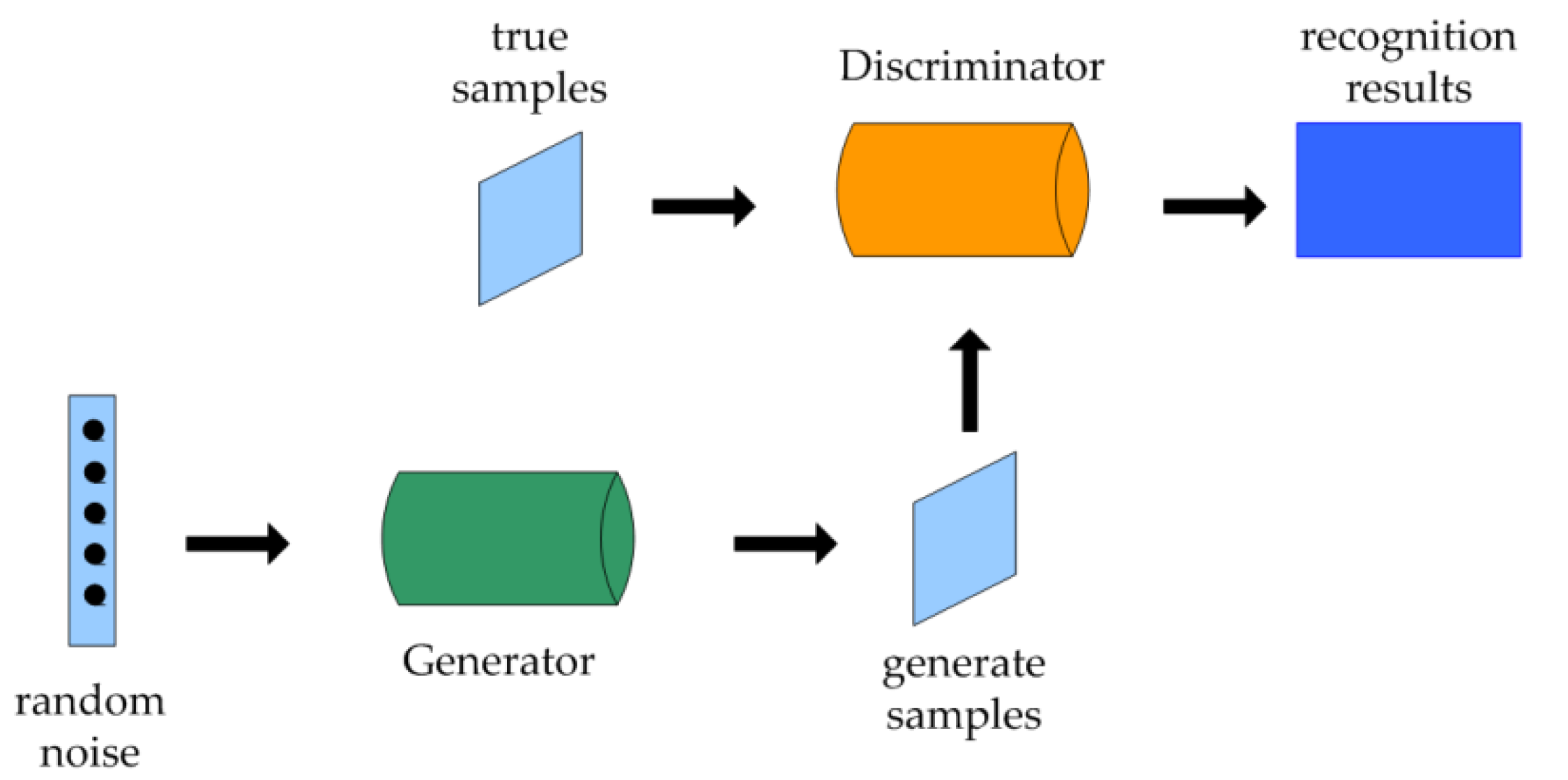
2.1. Generative Adversarial Network Model (GAN)

The generative adversarial network can learn the feature distribution of the input data through the game method and then generate the composite sample, whose feature distribution is close to the input data, so that the limited fault data sample set can be expanded. At present, in the field of data augmentation for fault diagnosis, the mainstream solution to the problem of unbalanced data sets is to use the generative adversarial network to expand the data set. The model is divided into two parts: generator G and discriminator D. The purpose of the generator is to generate pseudo-samples as close as possible to the real samples, and the purpose of the discriminator is to distinguish between real samples and pseudo-samples. The two compete, co-evolve, and finally reach Nash equilibrium. The network structure of the GAN is shown in Figure 1.

The training optimization objective of the GAN network, the GAN loss function, is as follows:

$$\underset{\mathrm{G}}{\min } \underset{\mathrm{D}}{\max } \mathrm{V}\left(\mathrm{D},\mathrm{G}\right){=\mathrm{E}}_{{\mathrm{X}~\mathrm{P}}_{\mathrm{data}\left(\mathrm{x}\right)}}\left[\log \mathrm{D}\left(\mathrm{x}\right)\right]{+\mathrm{E}}_{{\mathrm{X}~\mathrm{P}}_{\mathrm{z}}\left(\mathrm{x}\right)}\left[\log \left(1-\mathrm{D}\left(\mathrm{G}\left(\mathrm{z}\right)\right)\right)\right]$$

(1)

where E is the mathematical expectation, ${\mathrm{P}}_{\mathrm{data}}\left(\mathrm{x}\right)$ is the probability distribution of the real sample, and ${\mathrm{P}}_{\mathrm{z}}\left(\mathrm{z}\right)$ is the probability distribution of the generated sample. During the training of the model, the purpose of generator G is to mislead the judgment of discriminator D to generate as close to real data as possible, to make $\mathrm{D}\left(\mathrm{G}\left(z\right)\right)$ as large as possible, and $\mathrm{V}\left(\mathrm{D}, \mathrm{G}\right)$ as small as possible. The purpose of the discriminator D network is to enhance the classification ability of the true and false samples and to distinguish the real data and the generated data as correctly as possible; this is to say, $\mathrm{D}\left(\mathrm{x}\right)$ is the bigger the better, $\mathrm{D}\left(\mathrm{G}\left(z\right)\right)$ is the smaller the better, so that $\mathrm{V}\left(\mathrm{D}, \mathrm{G}\right)$ is as large as possible. When $\mathrm{D}\left(\mathrm{x}\right)=\mathrm{D}\left(\mathrm{G}\left(\mathrm{z}\right)\right)=0.5$, it is considered that the two have reached the Nash equilibrium of the game, then the training is over.

2.2. Auxiliary Classification Generative Adversarial Network Model (ACGAN)

The auxiliary classification generative adversarial network transforms the network structure of the generative adversarial network model and adds data label information to the generator and discriminator to generate results that meet the quality requirements. The model implements the variant architecture of the conventional GAN by using additional class labels of discriminators and generators, as shown in Figure 2. The class condition generation process can improve the quality of the generated data. In addition, the discriminator outputs specific class labels with auxiliary parts, so that the improved discriminator can distinguish various categories in addition to identifying data sources. This variant that combines class condition architecture and auxiliary networks for classification is called an auxiliary classifier generation adversarial network (ACGAN).

When compared with conventional GAN, ACGAN can generate high-quality data while providing label information. The generator network uses label information l and random noise z as input to generate data samples, ${\mathrm{X}}_{\mathrm{generated}}=\mathrm{G}\left(\mathrm{z}, \mathrm{l}\right)$, and the discriminator network receives a data sample as input and then outputs the authenticity and label of the sample. Therefore, its objective function is two independent log-likelihoods, corresponding to the true or false and correct label of the data sample, as follows:

$${\mathrm{L}}_{\mathrm{Source}}{=\mathrm{E}}_{{\mathrm{X}~\mathrm{P}}_{\mathrm{data}}}\left[\log \mathrm{p}\left({\mathrm{s}=\mathrm{real}|\mathrm{X}}_{\mathrm{real}}\right)\right]{+\mathrm{E}}_{\mathrm{Z}~\mathrm{P}\left(\mathrm{z}\right)}\left[\log \mathrm{p}\left({\mathrm{s}=\mathrm{generated}|\mathrm{X}}_{\mathrm{generated}}\right)\right]$$

(2)

$${\mathrm{L}}_{\mathrm{Class}}{=\mathrm{E}}_{{\mathrm{X}~\mathrm{P}}_{\mathrm{data}}}\left[\log \mathrm{p}\left({\mathrm{Class}=\mathrm{c}|\mathrm{X}}_{\mathrm{real}}\right)\right]{+\mathrm{E}}_{\mathrm{Z}~\mathrm{P}\left(\mathrm{z}\right)}\left[\log \mathrm{p}\left({\mathrm{Class}=\mathrm{c}|\mathrm{X}}_{\mathrm{generated}}\right)\right]$$

(3)

For the discriminator network, the training objective is to maximize the log-likelihood ${\mathrm{L}}_{\mathrm{Source}}+{\mathrm{L}}_{\mathrm{Class}}$, while the generator network is trained to maximize ${\mathrm{L}}_{\mathrm{Class}}-{\mathrm{L}}_{\mathrm{Source}}$. Because the auxiliary classification generative adversarial network adds label information, it can generate samples with higher quality than unsupervised GAN, so it is suitable for data augmentation tasks in fault diagnosis.

2.3. WGAN-GP Model

In order to solve the problem of training instability of classical GAN, the optimization goal of GAN is measured by Wasserstein distance instead of KL and JS divergence. Arjovsky et al. proposed the WGAN framework. The discriminator of WGAN distinguishes the classifier function between real data and generated data and measures the distance between them. This improvement provides an optimization direction for the generator, so that the generator training more purposeful and designed to improve the convergence speed and training stability [22]. The expression of Wasserstein distance is as follows:

$$\mathrm{W}\left({\mathrm{P}}_{\mathrm{data}}{, \mathrm{P}}_{\mathrm{z}}\right){=\sup \Vert f\Vert }_{\mathrm{L}\le 1}{ \mathrm{E}}_{{\mathrm{X}~\mathrm{P}}_{\mathrm{data}}}\left[\mathrm{f}\left(\mathrm{x}\right)\right]-{\mathrm{E}}_{{\mathrm{X}~\mathrm{P}}_{\mathrm{z}}}\left[\mathrm{f}\left(\mathrm{x}\right)\right]$$

(4)

Compared with KL divergence and JS divergence, Wasserstein distance can better compare the distribution differences between them. The former can only judge whether the two distributions are similar. The objective loss function of WGAN is:

$$\mathrm{V}\left(\mathrm{G},\mathrm{D}\right)=\underset{\mathrm{G}}{\min }\underset{\mathrm{D}\in 1-\mathrm{Lipschitz}}{\max }{ \mathrm{E}}_{{\mathrm{X}~\mathrm{P}}_{\mathrm{data}}}\left[\mathrm{D}\left(\mathrm{x}\right)\right]-{\mathrm{E}}_{{\mathrm{X}~\mathrm{P}}_{\mathrm{z}}}\left[\mathrm{D}\left(\mathrm{z}\right)\right]$$

(5)

WGAN cuts the weights of each layer of the discriminator to the range of [−c, c], so that the discriminator satisfies the 1 − L condition. However, this strategy not only limits the ability of the discriminator to fit complex data distribution, but also leads to the problem of vanishing gradient. In order to improve the performance of WGAN, Su X et al. proposed a generative adversarial network model based on gradient penalty and Wasserstein distance [23]. This model improves the loss function of WGAN and adds a gradient penalty term to the target loss function. The objective loss function of WGAN-GP is as follows:

$$\mathrm{L}=\stackrel{\mathrm{Meet} 1-\mathrm{L} \mathrm{conditions}}{\overbrace{{\mathrm{E}}_{{\mathrm{X}~\mathrm{P}}_{\mathrm{z}}}[\mathrm{D}(\tilde{\mathrm{X}})]-{\mathrm{E}}_{{\mathrm{X}~\mathrm{P}}_{\mathrm{data}}}\left[\mathrm{D}\left(\mathrm{X}\right)\right]}}+\stackrel{\mathrm{Gradient} \mathrm{penaity} \mathrm{term}}{\overbrace{{\mathsf{\lambda }\mathrm{E}}_{{\hat{\mathrm{X}}~\mathrm{P}}_{\hat{\mathrm{x}}}}\left[{\left(\Vert {\nabla }_{\hat{\mathrm{X}}}\mathrm{D}(\hat{\mathrm{X}}){\Vert }_2-1\right)}^2\right]}}$$

(6)

where $\mathsf{\lambda }$ is the penalty coefficient, $\hat{\mathrm{x}}$ is all $\mathrm{x}$ and $\tilde{\mathrm{x}}$ and their random mixing part in a training, $\hat{\mathrm{x}}=\mathsf{\epsilon }\mathrm{x}+\left(1-\mathsf{\epsilon }\right)\tilde{\mathrm{x}}$. The WGAN-GP algorithm flow is shown in Algorithm 1.

Algorithm 1: WGAN-GP algorithm flow

Parameters: gradient penalty coefficient $\mathsf{\lambda }$, the number of iterations $\mathrm{T},$ batch size m, Adam hyper-parameter ${\mathsf{\alpha }, \mathsf{\beta }}_1{, \mathsf{\beta }}_2$, initial discriminator parameter ${\mathsf{\omega }}_0$, initial generator parameter ${\mathsf{\theta }}_0$.

1: while $\mathsf{\theta }$ not convergent do 2: for t = 1, …, T 3:  for i = 1, …, m 4:   Sample x from real sample distribution ${\mathrm{P}}_{\mathrm{data}}$, random noise z from generator pre-random distribution ${\mathrm{P}}_{\mathrm{z}}$, random number $\mathsf{\epsilon }$ from uniform distribution [0, 1]

5:     $\tilde{\mathrm{x}}\leftarrow {\mathrm{G}}_{\mathsf{\theta }}\left(\mathrm{z}\right)$ 6:     $\hat{\mathrm{x}}\leftarrow \mathsf{\epsilon }\mathrm{x}+\left(1-\mathsf{\epsilon }\right)\tilde{\mathrm{x}}$ 7:     ${\mathrm{L}}^{\left(\mathrm{i}\right)}\leftarrow {\mathrm{D}}_{\mathsf{\omega }}\left(\tilde{\mathrm{x}}\right)-{\mathrm{D}}_{\mathsf{\omega }}\left(\mathrm{x}\right)+\mathsf{\lambda }{\left(\Vert {\nabla }_{\hat{\mathrm{x}}}{\mathrm{D}}_{\mathsf{\omega }}\left(\hat{\mathrm{x}}\right){\Vert }_2-1\right)}^2$ 8:  end for

9:  $\mathsf{\omega }\leftarrow \mathrm{Adam}\left({\nabla }_{\mathsf{\omega }}\frac{1}{\mathrm{m}}{{\displaystyle \sum }}_{\mathrm{i}=1}^{\mathrm{m}}{\mathrm{L}}^{\left(\mathrm{i}\right)}{, \mathsf{\omega }, \mathsf{\alpha }, \mathsf{\beta }}_1{, \mathsf{\beta }}_2\right)$

10: end for

11: Retrieve ${\left\{{\mathrm{z}}^{\left(\mathrm{i}\right)}\right\}}_{\mathrm{i}=1}^{\mathrm{m}}$ from the generator pre-randomly distributed ${\mathrm{P}}_{\mathrm{z}}$

12:  $\mathsf{\theta }\leftarrow \mathrm{Adam}\left({\nabla }_{\mathsf{\theta }}\frac{1}{\mathrm{m}}{{\displaystyle \sum }}_{\mathrm{i}=1}^{\mathrm{m}}-{\mathrm{D}}_{\mathsf{\omega }}\left({\mathrm{G}}_{\mathsf{\theta }}\left(\mathrm{z}\right)\right){, \mathsf{\theta }, \mathsf{\alpha }, \mathsf{\beta }}_1{, \mathsf{\beta }}_2\right)$

13: end while

3. Fault Diagnosis Framework of Rolling Bearing Using Improved ACGAN

3.1. PCA-ACWGAN-GP Model

ACGAN can control the direction of sample generation during the generation process by using an auxiliary classifier to generate high-quality results. However, due to the limited size of the convolution kernel, only the relationship between the local regions of the sample can be learned, the learning efficiency of the model is low, and details may be lost.

Based on the supervision idea of ACGAN, the self-attention mechanism [24] is added to G and D to help the model capture the relationship between the long-distance features of the sample; using Wasserstein distance to measure the difference between generated samples and real samples, an improved data augmentation model [25] is constructed to generate high-quality fault samples for rolling bearing fault diagnosis. The Wasserstein distance strictly limits the range of weights between −l and l by weight clipping, and when the weights updated in network training exceed the specified range, they are pruned to −l or l to satisfy the Kullback-Leibler Divergence constraint (hereafter referred to as the KLD). However, the restriction of weight clipping on network performance is more serious, and inappropriate parameter setting often causes gradient explosion or disappearance.

Therefore, KLD constraint is realized by introducing a gradient penalty term instead of weight clipping so as to avoid gradient explosion or disappearance due to unreasonable parameter setting. The KLD constraint restricts the gradient value of the discriminator below K. The gradient penalty is used to establish an additional loss term between the gradient and K. The following is the formula of the gradient penalty term ${\mathrm{L}}_{\mathrm{gp}}$:

$${\mathrm{L}}_{\mathrm{gp}}{=\mathsf{\lambda }\mathrm{E}}_{{\hat{\mathrm{X}}~\mathrm{P}}_{\hat{\mathrm{x}}}}\left[{\left(\Vert {\nabla }_{\hat{\mathrm{X}}}\mathrm{D}(\hat{\mathrm{X}}){\Vert }_2-1\right)}^2\right]$$

(7)

In the above formula, $\mathsf{\lambda }$ represents the penalty coefficient, $\nabla$ represents the gradient, and $\Vert ·{\Vert }_2$ represents the 2-norm, $\hat{\mathrm{x}}=\mathsf{\epsilon }\mathrm{x}+\left(1-\mathsf{\epsilon }\right)\hat{\mathrm{x}}$, where $\mathsf{\epsilon }~\mathrm{U}\left[0,1\right]$. Based on the original ACGAN loss function, plus ${\mathrm{L}}_{\mathrm{gp}}$, the improved ACGAN loss function is as follows:

$$\begin{array}{ll}{\mathrm{L}}_{\mathrm{Source}}{=\mathrm{E}}_{{\mathrm{X}~\mathrm{P}}_{\mathrm{data}}}& \left[\log \mathrm{p}\left({\mathrm{s}=\mathrm{real}|\mathrm{X}}_{\mathrm{real}}\right)\right]{+\mathrm{E}}_{\mathrm{Z}~\mathrm{P}\left(\mathrm{z}\right)}\left[\log \mathrm{p}\left({\mathrm{s}=\mathrm{generated}|\mathrm{X}}_{\mathrm{generated}}\right)\right]\\ & +{\mathsf{\lambda }\mathrm{E}}_{{\hat{\mathrm{X}}~\mathrm{P}}_{\hat{\mathrm{x}}}}\left[{\left(\Vert {\nabla }_{\hat{\mathrm{X}}}\mathrm{D}(\hat{\mathrm{X}}){\Vert }_2-1\right)}^2\right]\end{array}$$

(8)

$${\mathrm{L}}_{\mathrm{Class} }{=\mathrm{E}}_{{\mathrm{X}~\mathrm{P}}_{\mathrm{data}}}\left[\log \mathrm{p}\left({\mathrm{Class}=\mathrm{c}|\mathrm{X}}_{\mathrm{real}}\right)\right]{+\mathrm{E}}_{\mathrm{Z}~\mathrm{P}\left(\mathrm{z}\right)}\left[\log \mathrm{p}\left({\mathrm{Class}=\mathrm{c}|\mathrm{X}}_{\mathrm{generated}}\right)\right]$$

(9)

Principal component analysis (PCA) [26] can reduce the dimension of data while retaining some data features, reduce the complexity of subsequent work, and improve the calculation speed. Therefore, this paper combines principal component analysis with generative adversarial networks to improve the generation model. First, the one-dimensional time-domain signal is transformed into a two-dimensional grayscale image, and then the principal component analysis method is used to reduce the feature dimension of the real sample and extract the fault feature vector. Then, the feature vector is used as the input of the generator to improve the controllability of the samples generated by the generator. A generative adversarial network model (PCA-ACWGAN-GP model) based on two-dimensional grayscale images and a principal component analysis method is proposed.

3.2. PCA-ACWGAN-GP Framework

The PCA-ACWGAN-GP model framework is shown in Figure 3.

In the improved auxiliary classification generative adversarial network based on principal component analysis, the input z of the generator in the original network is improved, and PCA is used to reduce the dimension and extract the features of the real data. The obtained vector replaces the noise z that initially conforms to the normal distribution or uniform distribution and is input into the generator of ACWGAN-GP, which is used to train the generator to generate a pseudo-sample G(z). The generated G(z) and the real sample x are used as the input of discriminator D to train the discriminator to judge whether the data belongs to the real sample or the pseudo sample. The parameters of the generator and discriminator are adjusted by back propagation based on the results of the discriminator to minimize the objective loss function L.

The generator structure is shown in Figure 4. Transposed convolutional layer uses batch normalization and ReLU activation function, and output transposed convolutional layer uses tanh function as activation function. The feature vector z and label c obtained by the PCA dimension reduction of the two-dimensional grayscale image are connected to the input generator, and the dimension is expanded by 3-layer transposed convolution and input to the Self-Attention layer. The feature details are enriched by calculating the self-attention feature map, and then the generated fault grayscale image is outputted after 2-layer transposed convolution.

The discriminator model, shown in Figure 5, adopts a structure symmetrical to the generator model. In the output layer, the SoftMax function is used as an activation function to troubleshoot the data. In order to adapt to the gradient penalty term, the discriminator removes spectrum normalization and batch normalization. The LeakyReLU function is used as the activation function in each convolutional layer, and the Dropout layer is added to reduce the calculation parameters of the model and reduce the occurrence of over-fitting.

3.3. Model Training Process

The training process of PCA-ACWGAN-GP model includes four steps: generating pseudo samples, optimizing the generator, optimizing the discriminator, and the game between the generator and the discriminator.

The process of generating pseudo samples: set a batch size batch _ size = m, and randomly obtain m n-dimensional tensors from the Gaussian distribution, denoted as ${\left\{{\mathrm{z}}^{\left(\mathrm{i}\right)}\right\}}_{\mathrm{i}=1}^{\mathrm{m}}$. Input z into the generator through the expansion of the generator network, and finally output the data with the same shape and size as the real data, which is the generated pseudo-sample $\mathrm{G}{\left\{{\mathrm{z}}^{\left(\mathrm{i}\right)}\right\}}_{\mathrm{i}=1}^{\mathrm{m}}$.

Optimize the process of discriminator: after generating pseudo-samples, take the same batch size of the real sample ${\left\{{\mathrm{x}}^{\left(\mathrm{i}\right)}\right\}}_{\mathrm{i}=1}^{\mathrm{m}}$ mixed with pseudo-samples, and enter them together into the discriminator network to determine whether the input data is a real sample or pseudo-sample and get the corresponding loss values ${\mathrm{d}}_{\mathrm{real}}$ and ${\mathrm{d}}_{\mathrm{fake}}$. Using gradient penalty term and loss function, the discriminator network parameters are optimized using the Adam optimization method.

Optimized process of the generator: after completing an optimization of the discriminator, the generated pseudo sample $\mathrm{G}{\left\{{\mathrm{z}}^{\left(\mathrm{i}\right)}\right\}}_{\mathrm{i}=1}^{\mathrm{m}}$ is input into the discriminator to identify the authenticity. Keeping the discriminator network parameters unchanged, the generator network parameters are updated and optimized using the Adam optimization method.

After training this combined structure (that is, after an iteration), return to the beginning of the training and continue the loop until all epochs end. After enough epoch training, the generator and discriminator finally reach the Nash equilibrium of the game, which is embodied in the convergence of classification loss; this means that the model training is basically completed. The trained generator can generate rolling bearing vibration data of specified fault type according to the input label and can use the generated samples to enhance the initial unbalanced data set. Then, the classical classifier is trained by using the data-enhanced sample set to realize fault diagnosis.

After fully training the PCA-ACWGAN-GP, a batch of high-quality samples are generated and mixed with real samples to expand and enhance the data set. A 2D-CNN fault classifier is constructed to verify the data augmentation effect. Different data sets, including enhanced data sets, are used for 2D-CNN model training, and the data enhancement effect is reflected by comparing the training results.

4. Experimental Setup and Results Analysis

The experimental environment is Microsoft Windows 10, processor is Intel Core i7, memory capacity is 8 GB, graphics configuration is MVIDIA GeForce 920M, the language used is Python3.7, and the deep learning framework is Tensorflow1.14.

4.1. Data Set Partition and Data Preprocessing

The model is experimentally verified on the standard data set of rolling bearings of Case Western Reserve University (CWRU). As shown in Figure 6, the CWRU bearing experimental platform consists of a dual-horsepower motor, encoder, power dynamometer, and control electronic devices. The rolling bearing is nested on the shaft of the motor. Artificial damage is created on bearings using electric sparks, and each bearing is processed for only one type of fault, including roller, inner ring, and outer ring faults. Each fault has three different degrees of damage, including 0.007 inches, 0.014 inches, and 0.021 inches. There is also a healthy bearing without machining damage that contains a total of ten different fault labels. During the test, the vibration signal was collected under four different motor loads (0 horsepower, 1 horsepower, 2 horsepower, 3 horsepower); the frequency is 12 kHz.

Compared with the one-dimensional convolution network, the two-dimensional convolution network can effectively reduce the number of network training parameters, improve the convergence speed, and solve the problems of cumbersome training and loss of label information in traditional methods [27]. Therefore, this paper performs dimension conversion on one-dimensional time series signal using the signal-picture conversion method proposed in reference [28]. The specific calculation formula is shown in Formula 10.

$$\mathrm{P}\left(\mathrm{m}, \mathrm{n}\right)=\mathrm{round}\left\{\frac{\mathrm{L}\left[\left(\mathrm{m}-1\right)\mathrm{N}+\mathrm{n}\right]-\min \left(\mathrm{L}\right)}{\max \left(\mathrm{L}\right)-\min \left(\mathrm{L}\right)}\ast 255\right\}$$

(10)

In the formula: P represents the value of the m row and the n column in the two-dimensional grayscale image; L represents the value of one-dimensional time domain signal after single sampling, and its length is N2; N indicates that the size of the converted image is N ∗ N, corresponding to the length of L; the function round (x) represents rounding the data to ensure that the converted data is an integer valued [0, 255]. This is then converted to several 64 * 64 images, as shown in Figure 7.

Each fault label is randomly selected from 4096 consecutive points and repeated 400 times. Finally, a data set containing 4000 samples and 4096 data points per sample is obtained. After all the samples are converted into grayscale images, each fault category contains 400 image samples with a size of 64 * 64. The sample set used in the experiment is shown in

Table 1. Sample sets for experiments.

Fault Label	Fault Mode	Fault Size/Inch	Load/hp	Sample Size
0	Normal	-	0/1/2/3	400
1	Slight wear of inner ring	0.007		400
2	Moderate wear of inner ring	0.014		400
3	Severe wear of inner ring	0.021		400
4	Slight wear of rolling element	0.007		400
5	Moderate wear of rolling element	0.014		400
6	Severe wear of rolling element	0.021		400
7	Slight wear of outer ring	0.007		400
8	Moderate wear of outer ring	0.014		400
9	Severe wear of outer ring	0.021		400

.

To facilitate model training, the test samples are divided into two parts: training set and test set. First, 150 samples of each type of fault from the original experimental sample are randomly selected to form sample set A, containing a total of 1500 samples, and each label randomly selects 100 samples from the remaining samples to form sample set B, containing a total of 1000 samples. Sample set A, as the training set of PCA-ACWGAN-GP, is only used to train the PCA-ACWGAN-GP and generate samples; sample set B does not participate in the training process and is only used for the test process of the PCA-ACWGAN-GP in order to verify the training effect of the model. The division of sample sets is shown in

Table 2. Sample set division.

Fault Label	Sample Set A (Training Set)	Sample Set B (Test Set)
0	150	100
1~9	1350	900

.

4.2. Parameter Settings

If memory allows, try to use a larger batch size to increase the stability of the model. Set the batch size to 32, the iteration number epoch to 1000, the model gradient penalty coefficient λ to 10, and the input dimension of the generator to 100. Compared with the Adam algorithm, RMSProp algorithm can effectively alleviate the problem of unstable training, so RMSProp algorithm is selected as the optimizer in this experiment. The determination of network structure and hyperparameters is obtained by repeated comparison of experiments. In this paper, the proposed PCA-ACWGAN-GP model is compared with the ACWGAN-GP model without principal component analysis (PCA) and the ACGAN model to verify the improvement of the model generation effect of this algorithm.

4.3. Similarity Effect Analysis

Then, verify that the model can effectively fit the characteristics of fault samples and ensure the diversity of generated samples. After the training of the new model is completed, the data of 10 kinds of label faults of rolling bearings are enhanced to obtain the generated high-quality fault sample set. Figure 8 is the comparison between the 10 rolling bearing fault samples generated by the PCA-ACWGAN-GP model and the real samples. Figure 8 shows that the pseudo samples generated by the PCA-ACWGAN-GP model retain most of the important features of the real samples, making the pseudo samples highly similar to the real samples but not identical.

The similarity between the generated samples and the real samples is quantitatively described by Euclidean Distance (ED) and Cosine Distance (CD). ED judges the similarity degree by the distance between vectors; the closer the distance, the more similar. CD judges the similarity of vectors by the size of the vector angle. The closer the angle is to 0 degrees, the closer the cosine value is to 1, and the more similar the two vectors are. The mathematical expressions of Euclidean distance and cosine distance are:

$$\mathrm{d}\left(\mathrm{x}, \mathrm{y}\right)=\sqrt{{\left({\mathrm{x}}_1{-\mathrm{x}}_2\right)}^2+{\left({\mathrm{y}}_1-{\mathrm{y}}_2\right)}^2}$$

(11)

$$\cos \left(\mathrm{x}, \mathrm{y}\right)=\frac{\mathrm{x}\ast \mathrm{y}}{\left|\mathrm{x}\right|\left|\mathrm{y}\right|}=\frac{{{\displaystyle \sum }}_{\mathrm{i}=1}^{\mathrm{n}}{\mathrm{x}}_{\mathrm{i}}{\mathrm{y}}_{\mathrm{i}}}{\sqrt{{{\displaystyle \sum }}_{\mathrm{i}=1}^{\mathrm{n}}{\mathrm{x}}_{\mathrm{i}}{}^2\sqrt{{{\displaystyle \sum }}_{\mathrm{i}=1}^{\mathrm{n}}{\mathrm{y}}_{\mathrm{i}}{}^2}}}$$

(12)

Select 10 samples from each of the original ACGAN model and the PCA-ACWGAN-GP model and calculate the ED and CD with the real sample. The results are averaged, as shown in

Table 3. Comparison of generated samples of three models.

Fault Label	ACGAN		ACWGAN-GP		PCA-ACWGAN-GP
	ED	CD	ED	CD	ED	CD
0	0.55195	0.96437	0.53709	0.97003	0.45187	0.97517
2	0.56080	0.96095	0.53887	0.96250	0.46480	0.96491
4	0.60844	0.95151	0.52806	0.96346	0.50844	0.97150
6	0.76558	0.92160	0.86297	0.89894	0.76508	0.91161
8	0.59120	0.95339	0.56240	0.95920	0.51920	0.96339

. The samples generated by the PCA-ACWGAN-GP model are generally better than the original ACGAN model as the similarity with the real samples is higher.

4.4. Data Enhancement Effect Analysis

The trained ACGAN, ACWGAN-GP, and PCA-ACWGAN-GP are used to enhance the data of sample set A. In order to make the expanded sample set size 15,000, 1350 samples are generated under each fault label. The samples generated by ACGAN, ACWGAN-GP and PCA-ACWGAN-GP are formed into sample set 1, sample set 2, and sample set 3, respectively. These are randomly mixed with the initial training sample set A, and finally sample set 4 expanded by ACGAN, sample set 5 expanded by ACWGAN-GP, and sample set 6 expanded by PCA-ACWGAN-GP are formed. The expanded experimental samples are shown in

Table 4. Expanded experimental sample.

Fault Label	Generate Sample Set 1	Generate Sample Set 2	Generate Sample Set 3	Expanded Sample Set 4	Expanded Sample Set 5	Expanded Sample Set 6
0	1350	1350	1350	1500	1500	1500
1~9	12,150	12,150	12,150	13,500	13,500	13,500

. A classical CNN model is selected as the fault classifier to test the improvement of fault diagnosis accuracy by data enhancement. Since the two-dimensional grayscale image is used as the sample data, the 2D-CNN algorithm is used as the fault classifier to test the training effect of the extended sample.

Table 5. 2D-CNN network structure.

Number of Layers	Layer	Convolution Kernel/Filter/Step Size
1	2D convolution layer	5/32/5
2	Maximum pooling layer	2/-/2
3	2D convolution layer	3/64/3
4	Maximum pooling layer	2/-/2
5	2D convolution layer	3/128/3
6	Maximum pooling layer	2/-/2
7	2D convolution layer	3/256/3
8	Maximum pooling layer	2/-/2
9	Full connection layer	256-128
10	Full connection layer	128-1
11	SoftMax layer	-

shows the network layer structure of 2D-CNN [29].

Sample sets 4, 5, and 6 are used as the training sets of 2D-CNN. After the 2D-CNN is trained, use the trained 2D-CNN to classify the faults of sample set B and evaluate the fault diagnosis performance of 2D-CNN by precision, recall, F1 score, and accuracy. The calculation methods of the four indicators are as follows:

$$\mathrm{precision}=\frac{\mathrm{TP}}{\mathrm{TP}+\mathrm{FP}}$$

(13)

$$\mathrm{recall}=\frac{\mathrm{TP}}{\mathrm{TP}+\mathrm{FN}}$$

(14)

$$\mathrm{F}1=\frac{2\ast \mathrm{recall}\ast \mathrm{accuracy}}{\mathrm{recall}+\mathrm{accuracy}}$$

(15)

$$\mathrm{accuracy}=\frac{\mathrm{TP}+\mathrm{TN}}{\mathrm{N}}$$

(16)

where N is the total number of samples and TP indicates that the prediction result of the classifier is a positive sample, which is a positive sample, that is, the number of positive samples correctly identified. FP indicates that the predicted results of the classifier are positive samples, which are negative samples, that is, the number of false negative samples. TN indicates that the prediction result of the classifier is a negative sample, which is a negative sample, that is, the number of negative samples correctly identified. FN indicates that the prediction result of the classifier is a negative sample, which is a positive sample, that is, the number of missed positive samples. The closer the value of the four indicators is to 1, the better the effect is. The results are shown in

Table 6. Comparison of classification performance of 2D-CNN trained by three sample sets for sample B.

	ACGAN Expanded Sample Set 4			ACWGAN-GP Expanded Sample Set 5			PCA-ACWGAN-GP Expanded Sample Set 6
Fault Label	Precision Rate	Recall Rate	F1 Score	Precision Rate	Recall Rate	F1 Score	Precision Rate	Recall Rate	F1 Score
0	1.000	1.000	1.000	1.000	1.000	1.000	1.000	0.999	1.000
1	0.901	1.000	0.948	0.985	1.000	1.000	0.999	1.000	0.998
2	0.786	0.983	0.889	0.970	1.000	0.991	1.000	0.997	0.999
3	1.000	0.989	0.995	0.991	0.980	0.989	0.998	1.000	1.000
4	0.972	0.979	0.915	0.973	0.970	0.972	0.996	0.997	1.000
5	0.895	0.669	0.759	0.956	0.922	0.956	0.992	0.959	0.981
6	0.992	1.000	0.996	0.948	0.899	0.923	0.991	1.000	0.987
7	0.952	1.000	0.974	0.966	0.973	0.968	0.983	1.000	0.974
8	0.986	0.981	0.983	0.989	1.000	0.994	1.000	0.980	0.982
9	0.884	0.912	0.893	0.919	0.876	0.923	0.982	1.000	0.999
Accuracy	94.6%			97.8%			99.2%

.

It can be seen from Table 6 that when compared with the performance of ACGAN and ACWGAN-GP on four types of classification performance indicators, the performance index scores of the PCA-ACWGAN-GP extended sample set in multiple types of faults are significantly improved. The classifier trained by the sample set enhanced by PCA-ACWGAN-GP has been greatly improved in fault diagnosis accuracy. Especially in the fifth fault label, the extended sample set of PCA-ACWGAN-GP performs better in precision, recall, and F1 score. It shows that the PCA-ACWGAN-GP model with sample features as the generator input has a significant improvement in the quality of the generated samples and the fault diagnosis of the classifier.

In order to eliminate the influence of the classification performance of the 2D-CNN classifier itself on the results, this paper adds other commonly used classifiers for experiments, including the ELM [30], SVM [31], and LSTM algorithms [32]. The above methods are trained using sample set A and sample set 4, 5, and 6; fault diagnosis is performed on fault sample set B. The accuracy is shown in Figure 9. It can be seen from

Table 7. Data sets with different sample sizes.

Proportion of Sample	100%	90%	80%	70%	60%	50%	40%
Total number of training samples	1500	1350	1200	1050	900	750	600
Number of samples per category	150	135	120	105	90	75	60

that other classification algorithms are consistent with the performance of 2D-CNN. The fault diagnosis accuracy of the classifier trained by sample set 6 is obviously higher. This result proves that the results of 2D-CNN in this experiment can represent other fault classifiers and can effectively judge the data enhancement performance of the model.

4.5. Data Enhancement in Different Sample Scenarios

In order to study the influence of training set size on the ability of the PCA-ACWGAN-GP model to generate high-quality samples, the following different small sample scenarios are set up: by randomly reducing the samples, the training sample set A is gradually reduced from 100% to 40%. The specific construction is shown in Table 7.

The training sets of different sizes in Table 7 are used in the model training of the ACGAN, ACWGAN-GP, and PCA-ACWGAN-GP in turn. Each retraining model needs to clear all the data to avoid the influence of repeated training samples on the training results. After the three models have converged through enough epochs, the data augmentation for samples under each fault label and the generated sample set is randomly mixed with the training sample set to form a corresponding expanded sample set. In order to avoid the influence of the expanded sample size on the training effect of the classifier, the expanded sample set is uniformly set to 1500 samples for each type of fault. The extended sample sets are used to train 2D-CNN. After training, the fault diagnosis performance of sample set B is tested. The classification accuracy is shown in Figure 10. It can be seen from the figure that the fault diagnosis accuracy of the PCA-ACWGAN-GP extended sample set training classifier is still 97.3% when the minimum sample set is reduced to 40%. With the decrease in the number of training samples, the fault diagnosis accuracy of 2D-CNN trained by the PCA-ACWGAN-GP extended sample set decreases more slowly, and its fault diagnosis accuracy is better than ACGAN. The above conclusions show that PCA-ACWGAN-GP can effectively solve the problem of data quality degradation in the limited small sample scenario and effectively enhance the data of rolling bearing fault samples to improve the accuracy of fault diagnosis.

5. Conclusions and Future Research

Aiming at the problem of insufficient fault sample data in the research of rolling bearing fault diagnosis, this paper improves ACGAN and constructs a data enhancement model using a two-dimensional convolutional network instead of a full connection layer. First, the K-L condition is satisfied by adding a gradient penalty term to replace weight clipping. This method avoids the common problem of gradient explosion or disappearance in the GAN model training process, and significantly improves the stability of the network training process. The pooling layer is added to the discriminator network structure of the model, which effectively improves the ability of the discriminator network to extract features in multi-classification scenarios, enables the discriminator network to obtain stronger ability to distinguish true and false, and optimizes the Nash equilibrium state between the generator and the discriminator. Second, the generator of the generative adversarial network is improved. The one-dimensional time-domain signal is transformed into a two-dimensional grayscale image, then the principal component analysis method is used to reduce the feature dimension of the real sample, and the fault feature vector is extracted. Finally, the feature vector is used as the input of the generator to improve the controllability of the sample generated by the generator. A PCA-ACWGAN-GP data enhancement model is proposed and applied to the fault diagnosis of CWRU rolling bearings. The experimental results show that the model improves the ability of the generator to generate high-quality samples. In addition, it has good performance in a small sample scenario where the size of the training set is continuously reduced. In a word, accurate prediction and diagnosis of possible faults is an indispensable part of industrial production, and is conducive to sustainable development and has certain practical significance and demand.

Future research directions will relax the limitations of existing models in terms of the quality of generated samples and the number of real samples and optimize the model structure and improve computational efficiency.

References

1. Zhang, H.; Wang, R.; Pan, R.; Pan, H. Imbalanced Fault Diagnosis of Rolling Bearing Using Enhanced Generative Adversarial Networks. IEEE Access 2020, 8, 185950–185963. [Google Scholar] [CrossRef]
2. Mao, W.; Liu, Y.; Ding, L.; Li, Y. Imbalanced Fault Diagnosis of Rolling Bearing Based on Generative Adversarial Network: A Comparative Study. IEEE Access 2019, 7, 9515–9530. [Google Scholar] [CrossRef]
3. Shao, H.; Jiang, H.; Lin, Y.; Li, X. A novel method for intelligent fault diagnosis of rolling bearings using ensemble deep auto-encoders. Mech. Syst. Signal Pract. 2018, 102, 278–297. [Google Scholar] [CrossRef]
4. Levent, E.; Turker, I.; Serkan, K. A Generic Intelligent Bearing Fault Diagnosis System Using Compact Adaptive 1D CNN Classifier. J. Signal Process Sys. 2019, 91, 179–189. [Google Scholar]
5. Wang, L.; Wan, H.; Huang, D.; Liu, J.; Tang, X.; Gan, L. Sustainable Analysis of Insulator Fault Detection Based on Fine-Grained Visual Optimization. Sustainability 2023, 15, 3456. [Google Scholar] [CrossRef]
6. Attouri, K.; Mansouri, M.; Hajji, M.; Kouadri, A.; Bouzrara, K.; Nounou, H. Wind Power Converter Fault Diagnosis Using Reduced Kernel PCA-Based BiLSTM. Sustainability 2023, 15, 3191. [Google Scholar] [CrossRef]
7. Zeng, D.; Jiang, Y.; Zou, Y. Construction and verification of a new evaluation index for bearing life prediction characteristics. Shock Vib. 2018, 54, 94–104. [Google Scholar]
8. Lei, Y.; Jia, F.; Kong, D. Opportunities and challenges of mechanical intelligent fault diagnosis in big data era. J. Mech. Eng. 2018, 54, 94–104. [Google Scholar] [CrossRef]
9. Hu, T.; Tang, T.; Lin, R.; Chen, M.; Han, S.; Wu, J. A simple data augmentation algorithm and a self-adaptive convolutional architecture for few-shot fault diagnosis under different working conditions—ScienceDirect. Measurement 2020, 156, 107539. [Google Scholar] [CrossRef]
10. Zhou, F.; Yang, S.; Fujita, H.; Chen, D.; Wen, C. Deep learning fault diagnosis method based on global optimization GAN for unbalanced data. Knowl. Based Syst. 2020, 187, 104837.1–104837.19. [Google Scholar] [CrossRef]
11. Cheng, F.; Zhang, J.; Wen, C.; Liu, Z.; Li, Z. Large Cost-Sensitive Margin Distribution Machine for Imbalanced Data Classification. Neurocomputing 2017, 224, 45–57. [Google Scholar] [CrossRef]
12. Bousmalis, K.; Silberman, N.; Dohan, D.; Erhan, D.; Krishnan, D. Unsupervised Pixel-Level Domain Adaptation with Generative Adversarial Networks. In Proceedings of the 2017 IEEE Conference on Computer Vision and Pattern Recognition (CVPR), Honolulu, HI, USA, 21–26 July 2017; pp. 1–10. [Google Scholar]
13. Yu, Z.Y.; Luo, T.J. Research on clothing patterns generation based on multi-scales self-attention improved generative adversarial network. Int. J. Innov. Creat. Change 2021, 14, 647–663. [Google Scholar] [CrossRef]
14. Zhang, X.; He, C.; Lu, Y.; Chen, B.; Zhu, L.; Zhang, L. Fault diagnosis for small samples based on attention mechanism. Measurement 2022, 187, 110242. [Google Scholar] [CrossRef]
15. Xu, Z.; Jin, J.; Li, C. New method for the fault diagnosis of rolling bearings based on a multiscale convolutional neural network. Shock Vib. 2021, 40, 212–220. [Google Scholar]
16. Gong, W.; Chen, H.; Zhang, Z. Intelligent fault diagnosis for rolling bearing based on improved convolutional neural network. J. Vib. Eng. Technol. 2020, 33, 400–413. [Google Scholar]
17. Shao, S.; Wang, P.; Yan, R. Generative adversarial networks for data augmentation in machine fault diagnosis. Computing 2019, 106, 85–93. [Google Scholar] [CrossRef]
18. Gao, X.; Deng, F.; Yue, X. Data augmentation in fault diagnosis based on the Wasserstein generative adversarial network with gradient penalty. Neurocomputing 2020, 396, 487–494. [Google Scholar] [CrossRef]
19. Ding, Y.; Ma, L.; Ma, J.; Wang, C.; Lu, C. A Generative Adversarial Network-Based Intelligent Fault Diagnosis Method for Rotating Machinery Under Small Sample Size Conditions. IEEE Access 2019, 7, 149736–149749. [Google Scholar] [CrossRef]
20. Deng, M.; Deng, A.; Shi, Y.; Liu, Y.; Xu, M. Intelligent fault diagnosis based on sample weighted joint adversarial network. Neurocomputing 2022, 488, 168–182. [Google Scholar] [CrossRef]
21. Li, Z.; Zheng, T.; Yang, W.; Fu, H.; Wu, W. A Robust Fault Diagnosis Method for Rolling Bearings Based on Deep Convolutional Neural Network. In Proceedings of the 2019 Prognostics and System Health Management Conference (PHM-Qingdao), Qingdao, China, 25–27 October 2019; pp. 1–7. [Google Scholar]
22. Tang, W.; Tan, S.; Li, B.; Huang, J. Automatic Steganographic Distortion Learning Using a Generative Adversarial Network. IEEE Signal. Proc. Let. 2017, 24, 1547–1551. [Google Scholar] [CrossRef]
23. Su, X.; Liu, H.; Tao, L.; Lu, C.; Suo, M. An end-to-end framework for remaining useful life prediction of rolling bearing based on feature pre-extraction mechanism and deep adaptive transformer model. Comput. Ing. Eng. 2021, 161, 107531. [Google Scholar] [CrossRef]
24. Mi, Z.; Jiang, X.; Sun, T.; Xu, K. GAN-Generated Image Detection with Self-Attention Mechanism against GAN Generator Defect. IEEE J. Sel. Top. Signal Process. 2020, 14, 969–981. [Google Scholar] [CrossRef]
25. Ouchi, T.; Tabuse, M. Effectiveness of Data Augmentation in Pointer-Generator Model. ICAROB 2020, 25, 390–393. [Google Scholar] [CrossRef]
26. Cheng, P.; Chen, D.; Wang, J. Research on prediction model of thermal and moisture comfort of underwear based on principal component analysis and Genetic Algorithm–Back Propagation neural network. Int. J. Nonlin. Sci. Num. 2021, 22, 607–619. [Google Scholar] [CrossRef]
27. Shakya, A.; Biswas, M.; Pal, M. Classification of Radar data using Bayesian optimized two-dimensional Convolutional Neural Network. In Radar Remote Sensing; Elsevier: Amsterdam, The Netherlands, 2022; pp. 175–186. [Google Scholar]
28. Gao, S.; Wang, Q.; Zhang, Y. Rolling Bearing Fault Diagnosis Based on CEEMDAN and Refined Composite Multi-Scale Fuzzy Entropy. IEEE T. Instrum. Meas. 2021, 70, 3514908. [Google Scholar] [CrossRef]
29. Zhang, W. Research on Bearing Fault Diagnosis Algorithm Based on Convolutional Neural Network; Harbin Institute of Technology: Harbin, China, 2017. [Google Scholar]
30. Baranilingesan, I. Optimization algorithm-based Elman neural network controller for continuous stirred tank reactor process model. Curr. Sci. 2021, 120, 1324–1333. [Google Scholar] [CrossRef]
31. Cao, H.; Sun, P.; Zhao, L. PCA-SVM method with sliding window for online fault diagnosis of a small pressurized water reactor. Ann. Nucl. Energy 2022, 171, 109036. [Google Scholar] [CrossRef]
32. Mao, Y.; Qin, G.; Ni, P.; Liu, Q. Analysis of road traffic speed in Kunming plateau mountains: A fusion PSO-LSTM algorithm. Int. J. Urban Sci. 2021, 7, 87–107. [Google Scholar] [CrossRef]
Figure 1. Network structure of the GAN.
Sustainability 15 07836 g001
Figure 2. Network structure of ACGAN.
Sustainability 15 07836 g002
Figure 3. PCA-ACWGAN-GP model framework.
Sustainability 15 07836 g003
Figure 4. Structure of the generator.
Sustainability 15 07836 g004
Figure 5. Structure of the discriminator.
Sustainability 15 07836 g005
Figure 6. CWRU experimental platform.
Sustainability 15 07836 g006
Figure 7. Two-dimensional gray image of 10 types of faults.
Sustainability 15 07836 g007
Figure 8. Comparison between real samples and PCA-ACWGAN-GP generated samples.
Sustainability 15 07836 g008
Figure 9. Accuracy of each classifier after training.
Sustainability 15 07836 g009
Figure 10. Data Enhancement Performance in Various Small Sample Training Set Scenarios.
Sustainability 15 07836 g010