Article

Spatially Varying Impacts of Built Environment on Transfer Ridership of Metro and Bus Systems

1
School of Transportation and Logistics, Southwest Jiaotong University, Chengdu 611756, China
2
School of Transportation Engineering, East China Jiaotong University, Nanchang 330013, China
3
College of Air Traffic Management, Civil Aviation Flight University of China, Deyang 618307, China
*
Author to whom correspondence should be addressed.
Sustainability 2023, 15(10), 7891; https://doi.org/10.3390/su15107891
Submission received: 28 March 2023 / Revised: 6 May 2023 / Accepted: 9 May 2023 / Published: 11 May 2023
(This article belongs to the Special Issue Analysis in Urban Public Transportation Sustainability)

Abstract

:
Public transport, especially bus and metro, are fundamental elements of sustainable transport systems. However, a dearth of research has been devoted to exploring the correlation between the built environment and the intermodal transfer modes that link bus and metro. To address this research gap, this study aims to explore the relationship between the built environment and transfer ridership by examining transfer ridership across different modes. First, this study uses Automatic Fare Collection (AFC) and Automatic Vehicle Location (AVL) data collected in the city of Chengdu to identify the ridership of Metro-to-Bus (M-B) and Bus-to-Metro (B-M) transfer passengers using dynamic transfer time thresholds. A multi-scale geographically weighted regression model (MGWR) is employed to examine the impact of the built environment on M-B and B-M transfer modes and their scale effects. The findings demonstrate that the MGWR model is effective in capturing the spatial heterogeneity and scale effects of the interrelationships between different built environment factors in the M-B and B-M modes. Furthermore, the impact of different built environment factors on transfer ridership varies. In particular, the number of bus stops and lines have a more pronounced positive effect on promoting transfer ridership, while the density of non-motorway lanes has a significant negative effect. This research provides valuable insights for public transportation management and supports the seamless integration of bus and metro systems to optimize transfer services.

1. Introduction

As urbanization accelerates, the proliferation of private automobiles on roadways has engendered a plethora of problems, such as vehicular traffic congestion [1,2], air pollution [2,3], and fuel consumption [4,5]. In response to this challenge, the development of high-quality public transportation systems has become an indispensable imperative in metropolises with high population density [6]. The seamless transfer of ridership between different modes of transportation has become an indispensable aspect of modern public transportation systems. This study defines “transfers” as the process of changing between different modes of public transportation. Specifically, this study focuses on two types of transfer modes: metro-to-bus and bus-to-metro, as defined in the provided reference [7]. The transfer system’s topological structure comprises a metro network and a feeder bus network, the former typically being more efficient and having greater capacity, while the latter features flexibility with its multiple lines and directions. Given that a considerable number of passengers are unable to reach their final destinations directly, transfer between transportation modes becomes necessary, particularly for medium-to-long distance journeys [8]. In the realm of public transportation, unpleasant transfers are critical factors that can lead to negative user experiences due to their tendency to prolong travel time and reduce travel efficiency. Thus, it is paramount to identify the factors that impact transfer travel and establish a comprehensive understanding of the relationship between these factors and transfer ridership [9]. Improving the quality of transfers is crucial in enhancing the overall passenger experience and increasing the appeal of public transportation.
Numerous research studies have investigated the correlation between public transportation and the built environment, as well as socioeconomic characteristics [10,11,12,13,14]. These studies used quantitative methods to assess the impact of locally built environment factors on public transport, commonly known as the 5Ds: density, diversity, design, distance to transit, and destination accessibility [15,16,17]. However, the above literature focuses on a single mode of transport and neglects the impact of the built environment on intermodal transfer ridership. Furthermore, previous research has generally assumed spatial and temporal uniformity of each influencing factor, ignoring the presence of spatial heterogeneity. The fact is that a particular factor may have a greater influence in some places than in others. To ascertain the relationship more accurately between the built environment and public transport demand, it is crucial to apply spatial heterogeneity models that can determine the heterogeneous impact of the built environment on passenger flows from a global perspective [2].
To address these research gaps, this study aims to investigate the spatial heterogeneity of the impact of different built environment factors on M-B and B-M intermodal transport modes. First, this study uses Chengdu City’s large-scale Automated Fare Collection (AFC) and Automatic Vehicle Location (AVL) data to identify the transfer ridership between M-B and B-M modes. Different categories of built environment factors are obtained from various sources, such as the level of development around metro stations, the transport system, urban design, and the structural characteristics of the metro network. Second, this study uses the multiscale geographic weighted regression (MGWR) model to investigate the effects of diverse built environment factors on M-B and B-M transfer modes and makes comparisons with the traditional ordinary least squares (OLS) model and geographically weighted regression (GWR) model. Third, the MGWR model analysis results are utilized to investigate the spatial variability of the built environment factors’ influence on different transfer modes. This research provides insights into short-term public transport scheduling and future transfer station planning.
This paper is organized as follows. Section 2 provides a review of relevant studies in the literature. In Section 3 we describe the research materials, including the study area and relevant data, and outline the modelling framework and analytical methods used in this study. Section 4 presents the model results and their interpretation. Section 5 concludes the paper by highlighting its contributions and providing recommendations for future research.

2. Literature Review

Over the past few decades, transfer facilities have received increasing attention due to their central role in public transport systems. In the early stages, some researchers used survey data to investigate transfer behavior between the metro and other modes of transport. For example, Cherry et al. [18] used ordinal regression models to examine transfers from metro to bus in Bangkok and identified safety from crime and the distance between metro exits and bus stops as the two most important factors for passengers. Navarrete et al. [19] conducted a study to examine the distinctions in various transfer modes (metro-to-metro, metro-to-bus, bus-to-metro, and bus-to-bus) using self-reported evaluations of transfer experiences and associated factors such as walking distance and waiting times. However, these studies are susceptible to errors in data recording or self-reported responses. Moreover, in megacities with hundreds of metro stations and thousands of bus stations, it seems to be unfeasible to comprehensively identify and evaluate citywide metro-to-bus transfer behavior solely through surveys.
In the late 1990s, smart card payment systems were introduced in various cities, including Washington D.C. (Smartrip) and Tokyo (Suica), and subsequently proliferated to other metropolitan areas, serving as an essential component of the contemporary public transport fare collection system [20]. AFC data can be cost-effectively utilized by researchers to obtain travel information for multiple purposes [21]. A multitude of studies utilizing AFC data has focused on identifying transfer patterns between various public transportation systems. Specifically, Seaborn et al. [7] proposed a comprehensive definition of transfer behavior among different modes of public transportation (e.g., metro-to-bus, bus-to-metro, and bus-to-bus) using AFC data. The study’s findings were validated by comparison with long-term questionnaire survey data, and Seaborn et al. established a recommended range of transfer time thresholds for effective transfer identification [22,23,24]. Despite the advances in transfer identification made by these studies, the effect of transfer distance and time variation on identification results has not been adequately considered.
Metropolises focus on improving the built environment as a strategy to reduce the negative impacts of uncontrolled urbanization and car dependency on the transport system, the environment, and health [25]. The effects of the built environment on transit ridership are multifaceted. A substantial literature on transportation has examined the association between travel demand and the built environment, which is typically quantified through measures such as density, diversity, and design [26,27]. High density, mixed land use, small block structure with high intersection density, increasing availability of public transportation, and reduced distance to ideal destinations have generally been found to be positively associated with the promotion of public transportation and reduction of car dependence in urban areas [3,25,28]. Hence, a thorough investigation into the effects of the built environment on public transportation is essential [29].
Global regression models typically assume that the relationships between independent and dependent variables remain constant across the entire study area, without regard for spatial variation [30]. The OLS model, one of the most prominent global analysis techniques has been used by numerous researchers to analyze the impact of external factors on transit ridership at the station level [31,32,33]. This approach, however, neglects the spatial autocorrelation effect, whereby nearby geographic units tend to be more similar than those farther apart [34]. The presence of spatial autocorrelation directly contravenes the independence assumption of most standard parametric statistical procedures, leading to inconsistent parameter estimates across different units [35]. For instance, Zhu [36] suggested that the BE variables exhibit diverse associations with public transportation across various subdivided community samples in Hong Kong. Therefore, to account for the spatial non-stationarity of relationships, it is necessary to employ a spatially variable parameter model. As a result, the GWR model has been introduced and extensively applied [37]. Zhao utilized the GWR model to investigate commuting inequity and its determinants, while Li et al. [38] employed it to explore the impacts of fine-scale built environment factors on rail transit ridership in Guangzhou. It should be noted that the selection of search bandwidth in GWR has a direct impact on the model results. High-bandwidth estimations with large-effect scales are similar to those of the global model, whereas low-bandwidth estimations exhibit clear spatial variation [37]. However, GWR assumes uniform search bandwidths for all independent variables, neglecting the varying effect scales of different independent variables [28]. Additionally, GWR lacks robustness when confronted with parameter instability caused by outliers, multicollinearity (particularly with small sample sizes), and spatial autocorrelation [34]. To address this issue, Fotheringham [39] introduced the multiscale geographic weighted regression (MGWR) model, which overcomes the constraints of fixed bandwidths and accounts for the varying scale effects. This model has the capacity to minimize over-fitting by employing appropriate bandwidth and to alleviate the issue of collinearity, which is commonly encountered in GWR [40]. Therefore, given the successful validation of the MGWR, there is considerable potential for its use in investigating the spatial non-stationarity and scale effect of the built environment’s influence on public transport use.
To clarify the relationship between transfer passenger flow and various factors under different modes and contribute to the existing literature, this study investigates the variability of the effects of various factors on M-B and B-M transfer passenger flow. Large-scale smart card data, metro and bus station coordinates, and public transport GPS data are used to obtain a transfer-related dataset. The spatial disparities in the effects of determinants on transfer ridership for both bus and metro systems are examined using the MGWR model. This paper also highlights the spatial heterogeneity of the determinants of transfer ridership between bus and metro systems by examining the dissimilarities in the spatial effects of identical factors on transfer ridership by mode.

3. Materials and Methods

3.1. Study Area and Data

3.1.1. Study Area

Chengdu, a city in the Sichuan province of China, is a major economic hub in the Southwest region, with a total area of 14,335 square kilometres, including a built-up area of 949.6 square kilometres. As of December 2020, the city’s population was recorded at 20,937,700. The city is served by a comprehensive metro network comprising 7 lines, labelled 1, 2, 3, 4, 5, 7, and 10, with a total length of 518 km and 193 stations. The average daily passenger flow of the network is 3.75 million, underscoring its crucial role in the region’s transportation infrastructure. Furthermore, the city has an extensive bus system with 1028 bus lines, 11,551 bus stops, and a total distance coverage of 19,575.5 km, serving a staggering 1647.8 million passengers.
A buffer area is utilized to derive the pedestrian catchment area (PCA), with 800 m typically considered an acceptable distance for walking and thus applied to demarcate the PCAs of rail stations [41,42,43]. To account for overlapping regions in some buffer zones that may result in double or multiple counting of variables, the Tyson polygons have been employed, as shown in Figure 1.

3.1.2. Identification of Transfer Passenger

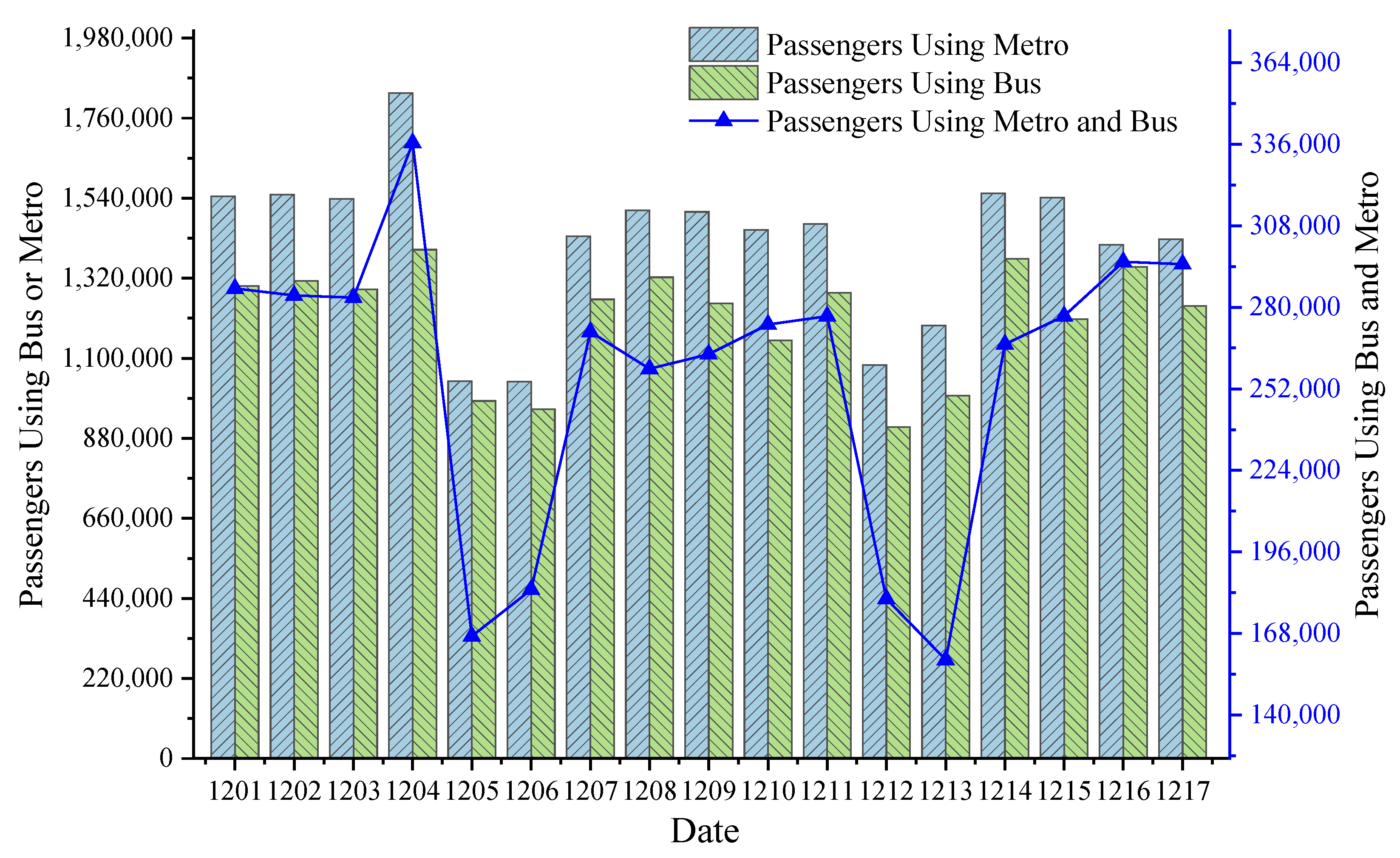
To obtain transfer ridership at the station level, this study used Automatic Fare Collection (AFC) data from both the bus and metro systems, as well as Automatic Vehicle Location (AVL) data from the bus system vehicles. Figure 2 displays the number of passengers using the bus or metro on the left vertical axis, as indicated by the bar graph, and the number of passengers using both modes of transport on the right-hand vertical axis, represented by the line graph. The graph reveals a consistent ridership pattern for both modes of transport and intermodal transfers during weekdays, with a significant decrease in ridership observed during weekends. Accordingly, this study utilizes AFC and AVL data solely from the 13 weekdays between 1 and 17 December 2020.
The AFC data for the metro system included card number, transaction time, and station number, resulting in 29,012,113 valid data after the removal of one-way cards and abnormal data. Similarly, the AFC data for the bus system contained fields such as card number, vehicle number, transaction time, and line number, with 31,958,456 valid data retained after excluding abnormal data. The AVL data from the bus vehicles provided vehicle number, line number, latitude, and longitude, running direction, speed, and recording time, resulting in a total of 296,648,677 valid data.
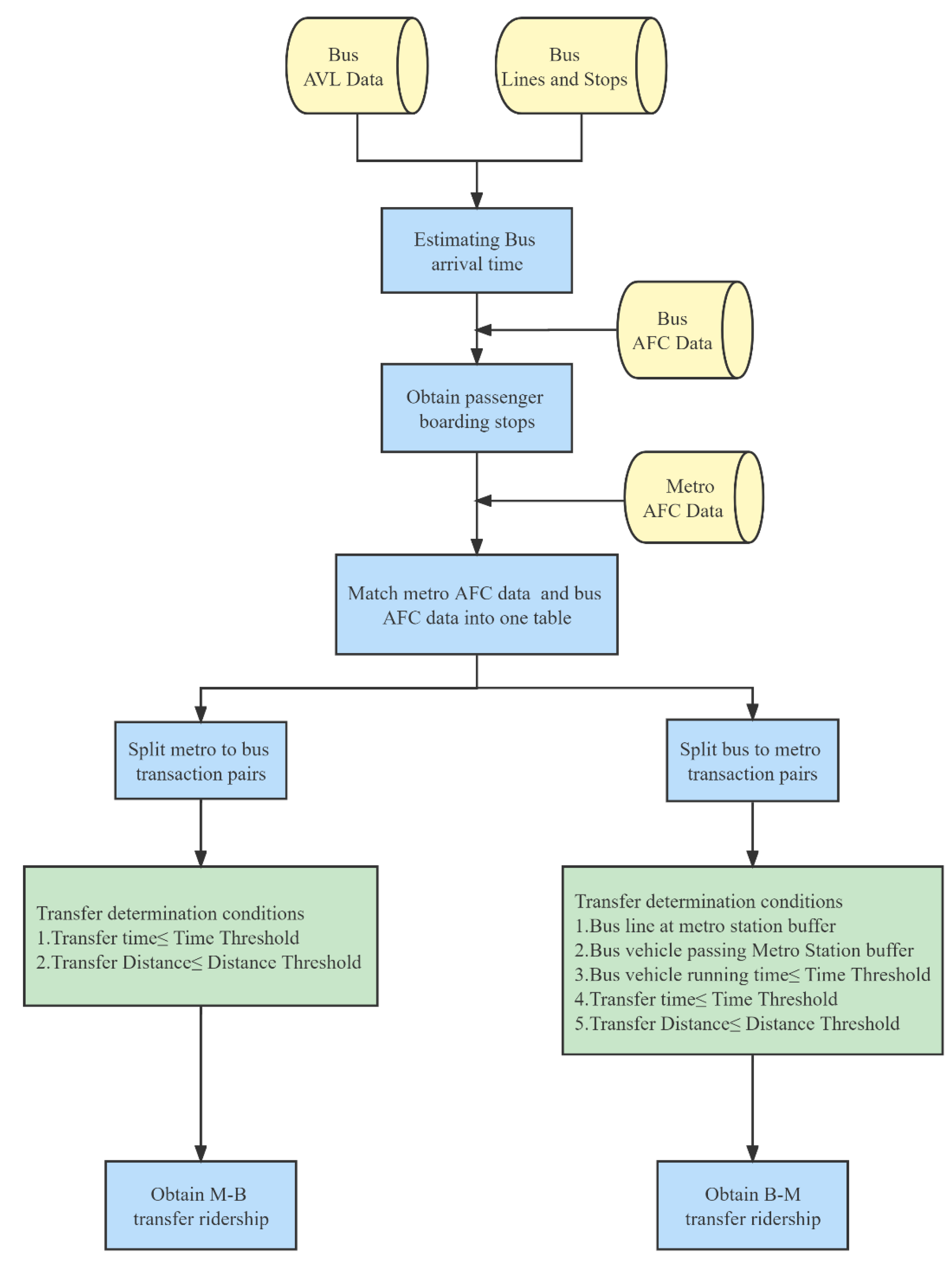
By analysing the data, this study was able to determine the Metro-to-Bus (M-B) and Bus-to-Metro (B-M) transfer ridership as the response variable. This study introduces a new methodology to detect transfers between metro and bus systems by utilizing dynamic spatiotemporal transfer thresholds. The proposed approach involves two key components: (1) inferring the boarding stops of bus passengers and (2) determining dynamic transfer time thresholds for M-B and B-M modes at various metro stations on different dates. The transfer ridership of M-B and B-M modes are then identified based on these transfer time thresholds and transfer distance thresholds. The transfer identification process is shown in Figure 3.
(1) Infer passengers’ boarding stop. Since there is no boarding information available in both bus AFC data and AVL data, and the AVL data may have positioning errors, matching the most recent AVL data with bus AFC data can lead to information loss and positioning errors [40,44]. To overcome this issue, we extract vehicle number and bus line information from both bus AFC data and AVL data and use recorded timestamps and geographic information technology to infer bus arrival information. This approach enables us to accurately determine the boarding point information of bus AFC data. Figure 4 and Equation (1) illustrate the specific process. To obtain the bus travel time around each stop, we set a distance threshold around it. However, GPS data is prone to positioning errors that cannot be eliminated. Rather than eliminating the GPS error, our objective is to infer the boarding record of the bus stop by matching bus arrival times. The activity recorded by the AFC data is typically performed after boarding the bus, which happens after the bus’s arrival timestamp. To reduce the impact of GPS errors, we extend the bus arriving time range by employing the first bus GPS time within the stop threshold as the bus arriving time, denoted as T 1 b V j . To infer the boarding records accurately, we consider the temporal and spatial conditions that impact the data. As the boarding transaction usually occurs after the bus reaches the stop and before it arrives at the next stop, we project the boarding transaction records in intervals consisting of every two adjacent bus arriving timestamps for each bus line. The boarding location in each interval is the bus stop corresponding to the start timestamp. To obtain the departure time of each bus, we rely on its arrival sequence along the bus line. Despite the gaps that GPS errors may cause in the arrival times, we aim to minimise their impact on the data.
T 1 b V j T p b F j T 1 b V j T 1 b V j = T 1 b V j + 1 δ 1
where T 1 b V j is the time at which vehicle V carrying passenger p arrives at bus stop j, T p b F j is the boarding time recorded in the AFC for passenger p at bus stop j, T 1 b V j is the time when vehicle V carrying passenger p departures at bus stop j, T 1 b V j + 1 is the time when vehicle V carrying passenger p arrives at stop j + 1, δ 1 represents the fixed flexible time and has been assigned a constant value of 30 s, as per the study conducted by Wu et al. [1].
(2) Transfer-related spatiotemporal parameters. The transfer mode of a passenger is determined by the combination of the metro station and bus stop, where the transfer distance is the distance between the two. Based on the given information by Gade et al. [45], the transfer distance d is calculated using the surface distance, as shown in Equation (2).
d = arccos cos x 1 cos x 2 cos y 1 y 2 + s i n x 1 sin x 2 2 π R / 360 × 1000
where x 1 and x 2 are the longitude coordinates of the metro station and bus stop, respectively; y 1 and y 2 are the latitude coordinates of the metro station and bus stop, respectively, R = 6371 km represents the mean radius of the Earth.
To accurately model transfer behaviour, it is essential to consider not only the spatial but also the temporal aspects. Previous studies have shown that the transfer time follows a log-normal distribution [7]. Based on the principles of probability and statistics, the probability density function for transfer time can be expressed as follows [46].
f Δ t i , t y p e K , S = 1 2 π Δ t i , t y p e K , S σ exp ( 1 2 σ 2 ln Δ t i , t y p e K , S μ ) 2
where Δ t i , t y p e K , S denotes the threshold value of the transfer time between the exit (entry) time at metro station i and the boarding (alighting) time of the bus at Sth hour on day K, type is M-B mode or B-M mode, μ is the mean of Δ t i , t y p e K , S , σ is the variance of Δ t i , t y p e K , S .
(3) Extraction of passenger sets for different transfer modes to determine transfer identification conditions. We form the sets of M-B transfer passengers and B-M transfer passengers by extracting two consecutive AFC data points before and after the passenger based on their card number and sorting the data chronologically.
To identify M-B transfer passengers, we use the passenger’s metro exit time and bus boarding time. The M-B transfer time threshold is determined as the 95th percentile of the cumulative distribution function of transfer time f 0.95 Δ t i , M B K , S . We begin by filtering out the elapsed time for the Sth hour of the day K at metro station i. Then, we sort the transfer times in ascending order and select the elapsed time ranked in the 95th percentile as the transfer time threshold for the Sth hour of the day K at metro station i, as shown in Equation (4).
d p , i j D T p b F j T p , i m F E x i t f 0.95 Δ t i , M B K , S
where d p , i j is the distance between metro station i and the bus stop j where passenger p gets on. T p b F j is the boarding time of passenger p at bus stop j as recorded in the AFC data, T p , i m F E x i t is the exit time of passenger p at metro station i as recorded in the AFC data.
To identify B-M transfer passengers, we need to obtain information about the passenger’s bus alighting stop, which is missing in the data. Therefore, we must refer to the passenger’s continuous record to determine their bus alighting stop before making the transfer determination. Equation (5) shows that in order to identify B-M transfer passengers, the bus line in the AFC data should be within the buffer of metro station i. If the bus line passes through multiple bus stops within the buffer, passengers are assumed to alight at the stop closest to the station i.
l = l p L i j l = min   d i j l
where l p is the bus line number of passenger p, L i is the set of bus lines in the catchment area of station I, j l is the bus stop containing bus line l, d i j l is the distance between the bus stop j l and metro station i.
To identify B-M passengers, we use Equation (6). We first check if the arrival time of the passenger’s bus vehicle V at the candidate bus stop falls between their boarding time and metro station entry time. Next, we ensure that the difference between their bus stop boarding time and metro station entry time is less δ 2 to avoid identifying rides that are too far apart in a day as multimodal. Finally, we verify that the difference between their bus alighting time and metro station entry time is less than the B-M dynamic transfer threshold.
T p b F < T p b V j l < T p , i m F E n t r y T p , i m F E n t r y T p b F δ 2 T p , i m F E n t r y T p b V n f 0.95 Δ t i , B M K , S
where T p b F is the time of boarding of the bus as recorded by passenger p in the AFC, T p b V j l is the arrival time at the stop j l of vehicle V carrying passenger p, T p , i m F E n t r y is the entry time at metro station i in the AFC of passenger p. δ 2 represents the time threshold between bus boarding time and metro entry time, defined as a fixed time interval of 50 min [47].

3.1.3. Explanatory Variables

Based on relevant literature and available data [48,49,50], this study presents a comprehensive system of indicators to assess the built environment surrounding metro stations, which is based on four categories, including the level of development around the station, the transportation system, the urban design, and the structural characteristics of the metro network. The system includes nine explanatory variables, of which one is categorical and eight are continuous. Their definitions and descriptive statistics are shown in Table 1.
The ArcGIS was used to derive the built environment variables within the buffer zone of the metro station, while the Amap application program interface (https://www.amap.com/) was used to collect the POI data in Chengdu on 17 December 2020. Of the POI categories, nine were chosen, namely restaurants, residences, shopping facilities, hospitals, hotels, schools, commercial establishments, government offices, and parks, all of which were deemed influential in transfer behaviour. These POI categories were used to calculate the land use mix as in Equation (7).
E i = P i k ln P i k ln N i ,
where E i is the land use mix within the catchment area of station i, P i k is the number of POIs in category k within the catchment area of station i, and N i is the number of different POI data within the catchment area of station i.
The accessibility of stations was then calculated using Equation (8), based on the metro line network data provided by the Chengdu Rail Transit Group.
A i = 1 Z i = n 1 i = 1 i i n g i i ,
where A i is the accessibility of station i, g i i is the shortest distance from station i to station i′, and Z i is the average distance from metro station i to other stations.

3.2. Spatial Autocorrelation

Before applying the spatial regression model, it is necessary to assess the spatial autocorrelation of variables spatial regression model. A common measure of global spatial autocorrelation is Moran’s I index, which can be defined mathematically as follows:
I = n i = 1 i i n i = 1 i i n c i i i = 1 i i n i = 1 i i n c i i ( θ i θ ¯ ) ( θ i θ ¯ ) i = 1 n ( θ i θ ¯ ) 2
where n is the number of metro stations indexed by i and i′, c i i is an element of a spatial weight matrix c with zeros on the diagonal, which expresses the relationships between neighbouring stations, and θ i and θ ¯ denote the independent variable at station i and the mean of θ , respectively.
Moran’s I index ranges from −1 to 1, where negative values indicate spatial dispersion, and positive values indicate spatial autocorrelation. If the observed value is significantly lower than −1/(N − 1), it indicates spatial dispersion among stations. Conversely, values significantly higher than −1/(N − 1) indicate a stronger degree of spatial autocorrelation. If Moran’s I index equal zero, it indicates a certain degree of randomness in the variable [48].
In general, the Z-score is used to test the statistical significance of Moran’s I index, which is calculated as follows:
Z I = I E ( I ) V a r ( I )
where E ( I ) and V a r ( I ) are the expectation and standard deviation of the global Moran’s I index, respectively.
A positive Moran’s I index indicates a high degree of spatial clustering, while a negative value indicates a more dispersed spatial distribution. The statistical significance of Moran’s I index is typically assessed using a pseudo-p-value. If the pseudo-p-value is less than 0.05, the global Moran’s I index is considered significant at the 95% confidence level, indicating that the variable under consideration is spatially correlated. Conversely, a pseudo-p-value greater than or equal to 0.05 suggests that the variable is likely to be randomly distributed and independent of spatial location [51].

3.3. Global Model

The OLS regression model is used to examine the relationship between several explanatory variables and a response variable [52]. The optimal regression coefficients for research data can be obtained by minimising the sum of squared errors [53], as shown in Equation (11).
y i = β 0 + β x i + ε i
where for the station i , y i is the M-B or B-M transfer ridership, β 0 is the intercept, x i is the vector of candidate variables in this study, β is the regression coefficient, and ε i is the random error term.
However, OLS fails to account for the potential spatial dependence among observations with independent influencing factors at the station level, which runs counter to the reality that the determinants of metro usage are often spatially correlated. Therefore, OLS was considered inadequate for modelling variable interactions.

3.4. Local Models

3.4.1. Geographically Weighted Regression (GWR)

Global regression models assume stationarity and spatial invariance in the relationship between the dependent and independent variables, ignoring spatial heterogeneity. As a result, coefficients obtained from global estimations show insignificant spatial variation [54]. It is essential to use local models that allow parameters to vary over space. The GWR model, which assumes non-stationarity in the relationships between explanatory and response variables, can estimate location-specific parameters as expressed in Equation (12).
y i = β 0 ( u i , v i ) + k = 1 n β k ( u i , v i ) x i k + ε i
where for the station i , ( u i , v i ) represents the geographical coordinates, β 0 ( u i , v i ) is the intercept term, n is the total number of independent variables, and x i k is the k th independent variable of the metro station.

3.4.2. Multiscale Geographically Weighted Regression (MGWR)

GWR has an inherent limitation in that it assumes that all modelled processes operate at the same spatial scale (same bandwidth), which is inconsistent with the fact that the scale of all explanatory determinants is not always the same in space. Thus, it may lead to biased results for selected variables involving different spatial processes. To overcome this limitation, a new method called MGWR is proposed [39]. It allows each relationship to be varied based on a different spatial scale parameter, and an optimal bandwidth is calculated for each parameter surface. The formulation of MGWR can be expressed as Equation (13).
y i = β 0 ( u i , v i ) + k = 1 n β b w k ( u i , v i ) x i k + ε i ,
where β b w k ( u i , v i ) indicates the bandwidth used for calibration of the k th independent variable, and the meaning of other parameters is the same as the ones in GWR.
In this study, the adaptive bi-square spatial kernel weighting approach was used to estimate the kernel bandwidth for GWR and MGWR. The golden bandwidth search method was used to determine the uniform and locally varying bandwidths for GWR and MGWR. The corrected Akaike information criterion (AICc) value was used as the optimization criterion to calculate the optimal bandwidth.

4. Results and Discussion

4.1. Validation and Analysis of Transfer Results

4.1.1. The Accuracy of Transfer Identification

Based on the dynamic threshold transfer identification method used for metro and bus, it is crucial to ensure the accuracy of both the arrival time of the bus and the number of passengers boarding. To verify this characteristic, this study conducted a following car survey during the morning and evening peak hours on 17 December 2020, comparing the arrival times and boarding numbers of vehicles on bus lines 49, 56, and 73 at different frequencies with the inferred results, as shown in Table 2.
During the survey, volunteers manually recorded the opening time of bus vehicle doors when arriving at each station (for non-stopping stations, the time of passing the station was used as the arrival time), obtained the arrival time of the bus vehicle, and recorded the number of passengers boarding at each bus station. The time interval refers to the interval between the actual arrival time of the vehicle and the estimated arrival time. The maximum number of error stops is the maximum number of error stops in a complete operation.
The results show that the method used in this study provided accurate extrapolation of 508 bus stops, with an average difference between the actual and extrapolated arrival time of no more than 20 s. The maximum error observed throughout the survey for the 3 lines was limited to 1 stop, leading to a total of 17 erroneous stops, while the accuracy of the extrapolation of boarding stops amounted to 96.65%. Moreover, the number and time of boarding in certain lines were inferred with an error rate of no more than 3%. Hence, this method can effectively ensure the accuracy of bus vehicle arrival time and boarding passenger numbers, thus providing robust data support for subsequent metro and bus transfer identification outcomes.

4.1.2. Transfer Passenger Flow Characteristics

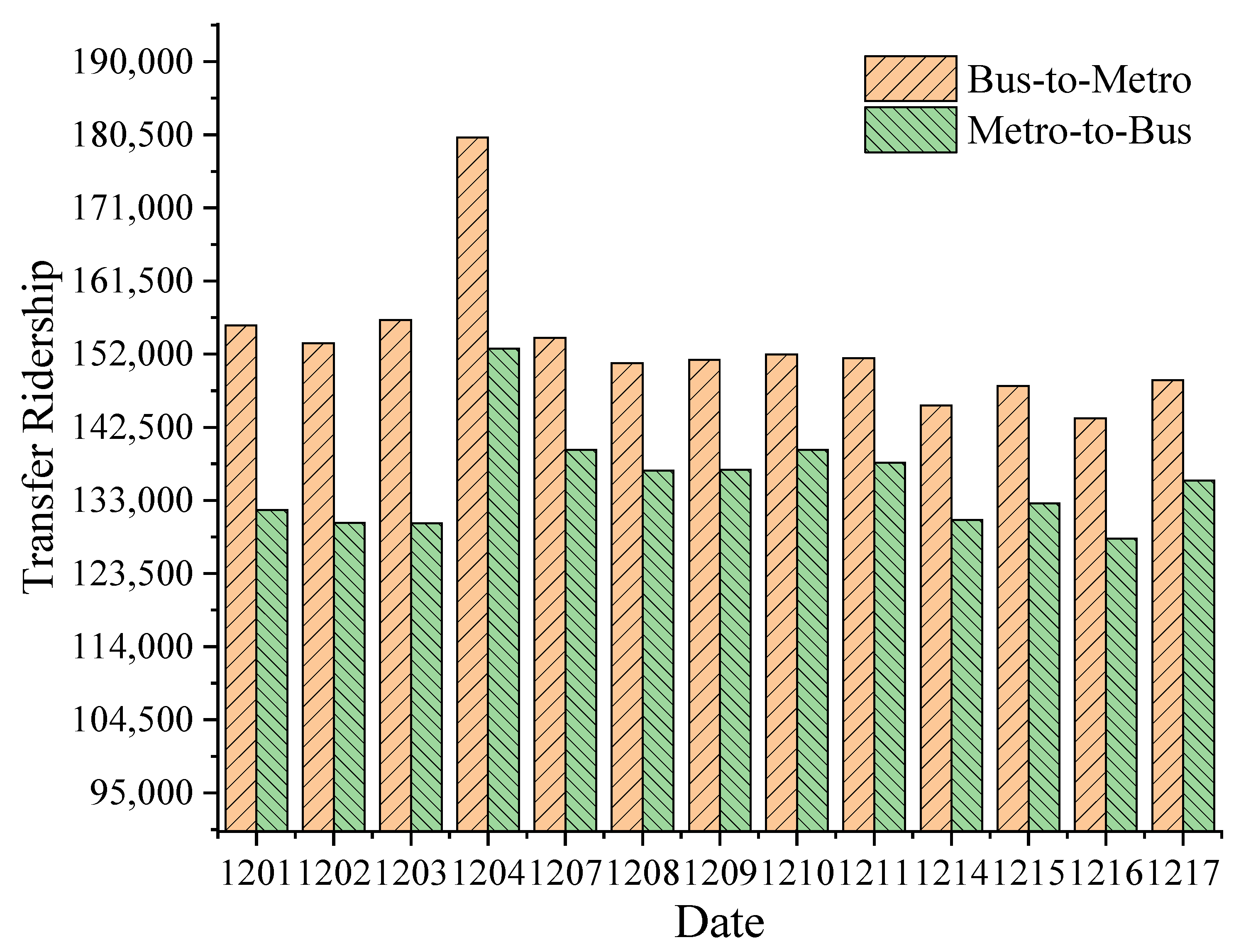
This study illustrates the results of validating and analyzing the identified transfer ridership between the B-M and M-B modes during 13 weekdays from 1 December to 17 December 2020 in Chengdu, as shown in Figure 5. The figure reveals a consistent pattern in the daily transfer ridership for both modes, with an initial increase, followed by a decline, and eventually reaching a relatively stable level. During the observation period, the 4th of December recorded the highest B-M and M-B transfer ridership of 180,141 persons and 157,745 persons, respectively, while the 16th of December recorded the lowest transfer ridership of 140,942 persons and 122,746 persons for B-M mode and M-B mode, respectively. The temporal distribution of B-M and M-B transfer ridership on different weekdays shows a high degree of correspondence with the distribution of metro and bus ridership.
In Figure 5, it can be observed that during the study period, M-B transfer ridership is lower than B-M transfer ridership. There are several reasons for this trend. Firstly, it can be attributed to the preference of people for the metro as their primary mode of transportation. As shown in Figure 2, the number of metro passengers is greater than the number of public transport passengers daily, which is consistent with the findings of Liao et al. [55]. Secondly, from the perspective of transfer convenience, the transfer from the bus to the metro is more attractive as there is no waiting time for the bus to arrive at the metro station, making it more convenient [56]. Finally, from an urban land use perspective, workplaces are mainly located in the inner city. Passengers travelling long distances for work purposes may opt to take the bus to reach the metro station for transfer. However, when travelling back home, the timeliness requirements are lower, and alternative transportation options are available for the connection.
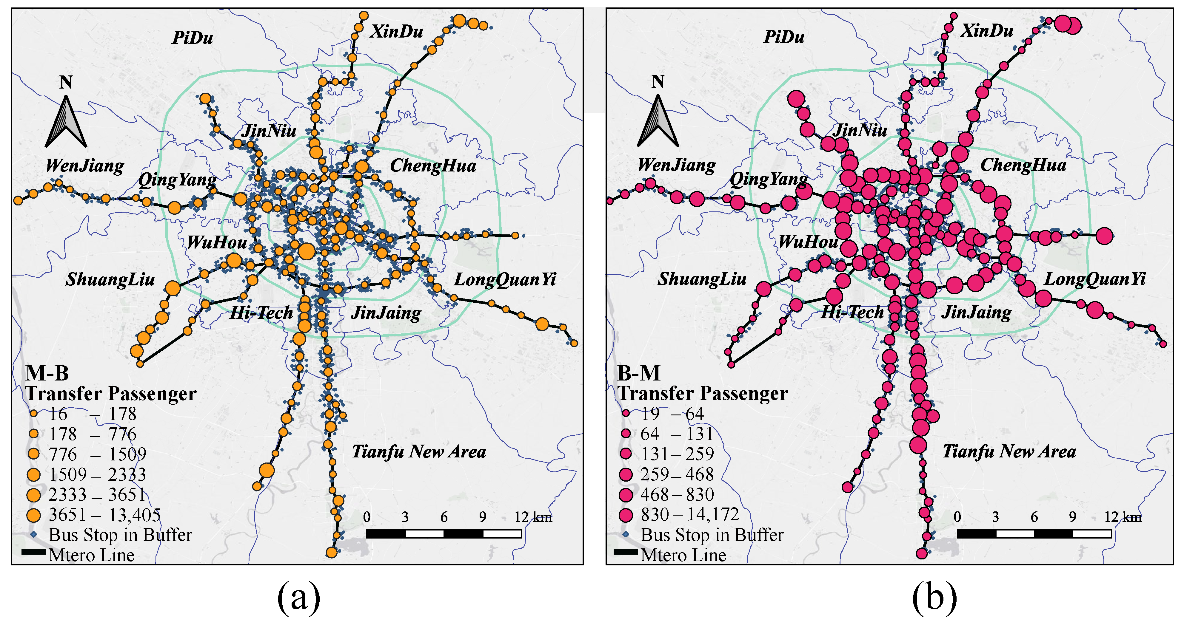
Subsequently, the study selected the average number of transfer passengers at 13 metro stations on weekdays as the dependent variable to investigate the spatial distribution of transfer passenger flows, as shown in Figure 6. Figure 6a,b shows that there are noticeable differences in the spatial distribution of B-M and M-B transfer ridership. Regarding the transfer ridership values, it was observed that the average daily transfer ridership at metro stations varies significantly, ranging from 16 to 13,405 in the M-B mode and from 19 to 14,712 in the B-M mode. Specifically, the B-M transfer ridership is more concentrated than the M-B transfer ridership with a higher concentration of B-M transfer ridership in the vicinity of the 4th Ring Road, particularly along Line 7, which encircles the 2nd Ring Road. Conversely, M-B transfer ridership is relatively high at the ends of several metro lines, such as Line 1 and Line 3.

4.2. Model Results

4.2.1. OLS Model Results

Before constructing the OLS model, the multicollinearity and spatial autocorrelation between the explanatory variables needs to be tested. In this study, the variance inflation factor (VIF) and the Pearson correlation coefficient were used to assess the degree of multicollinearity between the variables.
The correlation coefficient between the variables is calculated, and if it is greater than 0.7, the two variables are considered highly correlated and therefore removed from consideration. The explanatory variables were calculated to be correlated less than 0.7. Then, we computed the VIF values and conducted spatial autocorrelation tests for all the variables. The resulting VIF values were all found to be below 10, with most even below 5, indicating a state of low multicollinearity between the selected variables and thus providing a safer threshold for their inclusion [57,58]. Table 3 shows the results of the VIF and Moran’s I index test for each variable. The presented table shows that the VIF values of the explanatory variables in both the M-B and B-M models range from 1.12 to 4.37, which are all below the optimal threshold of 5. This observation suggests that there is no multicollinearity between the explanatory variables. All explanatory variables show significant spatial autocorrelation with the dependent variables (p-values < 0.05), and the positive Z-values indicate the presence of a discernible spatial clustering pattern for the variables.
In addition, spatial autocorrelation measures the spatial dependence of a given element based on its location and numerical value. The null hypothesis assumes no spatial correlation, but it is rejected based on the results [59]. The significant p-values of all variables demonstrate a strong spatial correlation, and the positive Z-value indicates the spatial clustering of each variable. These findings suggest that the global OLS model is insufficient to analyze the relationship between transfer ridership and dependent variables effectively. Thus, it is recommended to utilize a geographically weighted regression cluster model to investigate the spatial heterogeneity of the data.
The results of the OLS model are shown in Table 4. The explanatory variables that were selected for this study were all significant. For the M-B transfer mode, the variables of Station Accessibility and Non-motorized lane are statistically significant at the 0.01 level. For the B-M transfer mode, the variables of the City Center and Non-motorized lane are statistically significant at the 0.01 level. Additionally, the Non-motorized lane exhibits a negative correlation with both transfer modes. The three coefficients with the largest magnitude are Bus Line, Station Accessibility, and Bus Stop. Notably, the coefficient of the Bus Line and Bus Stop are positively associated with the bus system and has the most pronounced effect on the transfer ridership. This outcome aligns with the previous results reported by Wu et al. [47].

4.2.2. Model Comparison and Performance

To compare the results of the global regression model, we used the OLS model with all variables to investigate the effect of spatial variability of the explanatory variables. The data were calculated and fitted using both the MGWR model and the GWR model using MGWR2.0 software. The means and standard deviations (S.D) of the regression coefficients associated with GWR and MGWR were calculated for the M-B and B-M transfer modes, as shown in Table 5.
To explore the relationship between the explanatory and response variables that vary in space and to account for the spatial autocorrelation issue, the GWR model and the MGWR model were employed, as shown in Table 6. Upon comparing the global OLS model, GWR model, and MGWR model for both B-M and M-B transfer modes, it was determined that the MGWR model outperformed the GWR and OLS models in terms of the model evaluation parameters AICc, R2 and Adj.R2. In the B-M mode, the MGWR model showed a 13.34% decrease in AICc and a 42.28% decrease in Adj.R2 compared to the GWR and OLS models, whereas the latter two models showed an 8.6%- and 4.07-fold increase in AICc and Adj.R2, respectively. Similarly, in the M-B mode, the MGWR model showed a 15.5% decrease in AICc and a 40.2% decrease in Adj.R2 compared to the GWR and OLS models, while the latter two models showed an increase of 5.77% and 5.16 times for AICc and A Adj.R2, respectively. Based on the results of the above indicators, it can be concluded that the MGWR model provides better estimates than the GWR model, thus more accurately characterizing the spatial heterogeneity of the effects of the built environment variables on B-M and M-B transfer ridership, as well as their scale effects.
While both local models show significant improvement in fitting performance compared to the global models, the MGWR model exhibits superior goodness of fitness to GWR, owing to its ability to assign an optimal bandwidth to each independent variable. In this study, the number of metro stations was 193. The choice of bandwidth value for a variable reflects its spatial influence, with a value closer to 193 indicating a more global impact and less spatial variability, and vice versa.
The bandwidth values used for GWR and MGWR models are presented in Table 7. For either B-M or M-B transfer modes, the GWR has a best-fitting bandwidth of 79, which represents the average range of action of the variables on a spatial scale. In the B-M and M-B transfer modes, variables Metro Line, Mixed land use, and Non-motorized lane show larger scales of action with values of 156, 44, and 138, respectively. This indicates that their impact on transfer ridership shows less spatial heterogeneity. Furthermore, for B-M, Bus Line equals 47 for 24.35% of the metro stations, and for M-B, Bus Line equals 46 for 19.68% of the metro stations, both utilizing the narrowest bandwidths of the modes. This suggests that there is a higher degree of spatial heterogeneity in the impact of the two variables on the corresponding transfer ridership.

4.2.3. MGWR Model Results

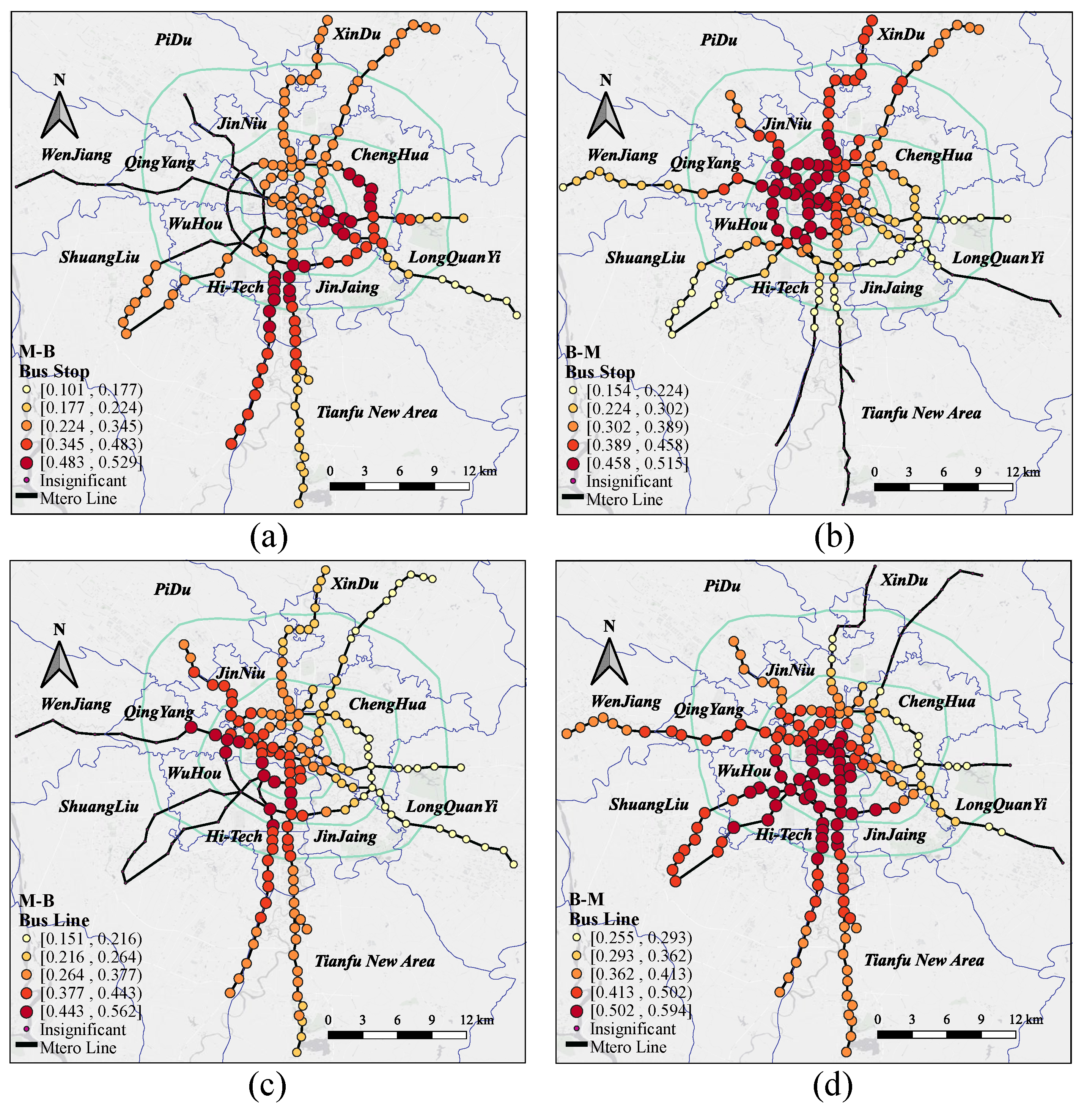
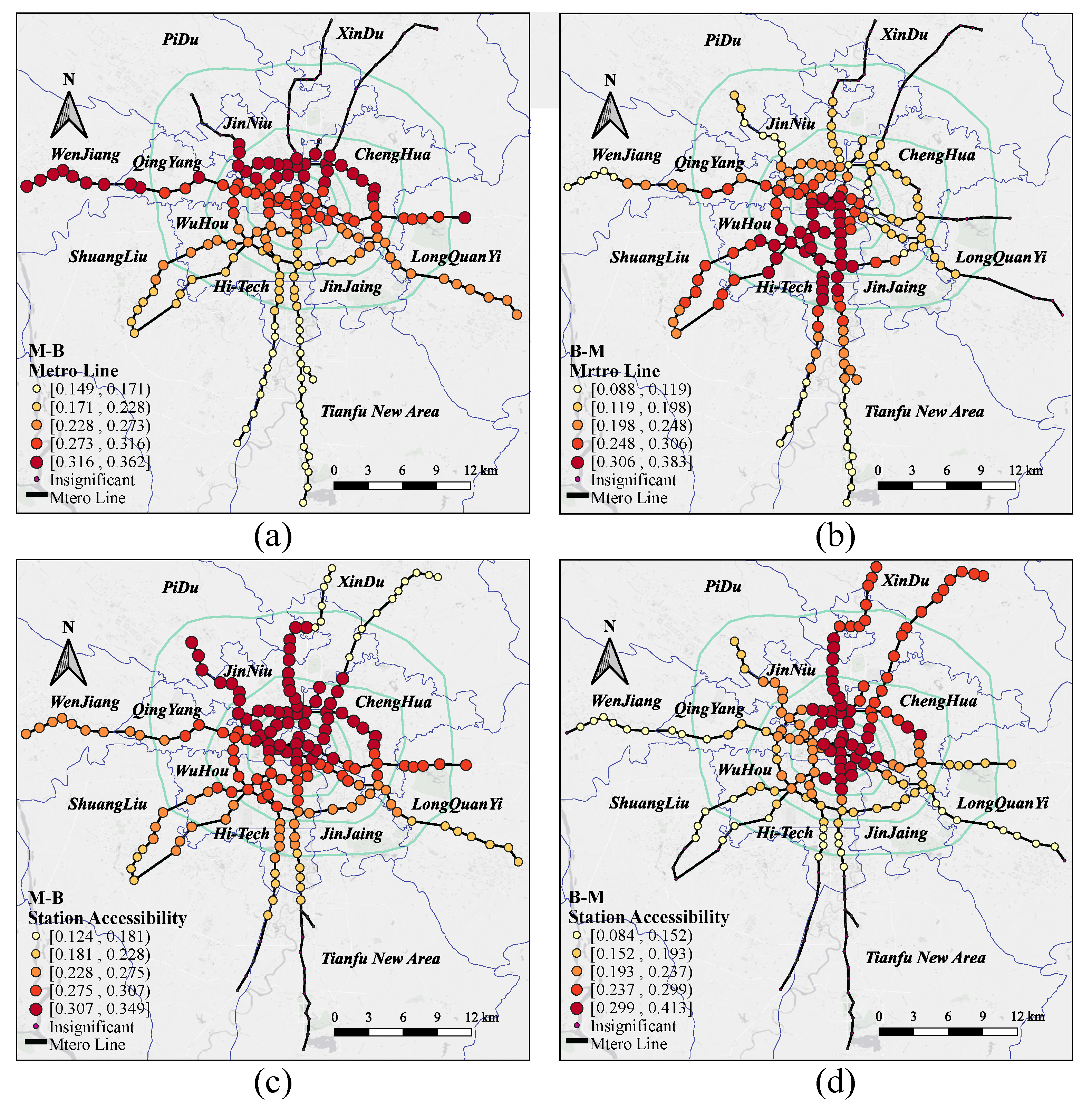
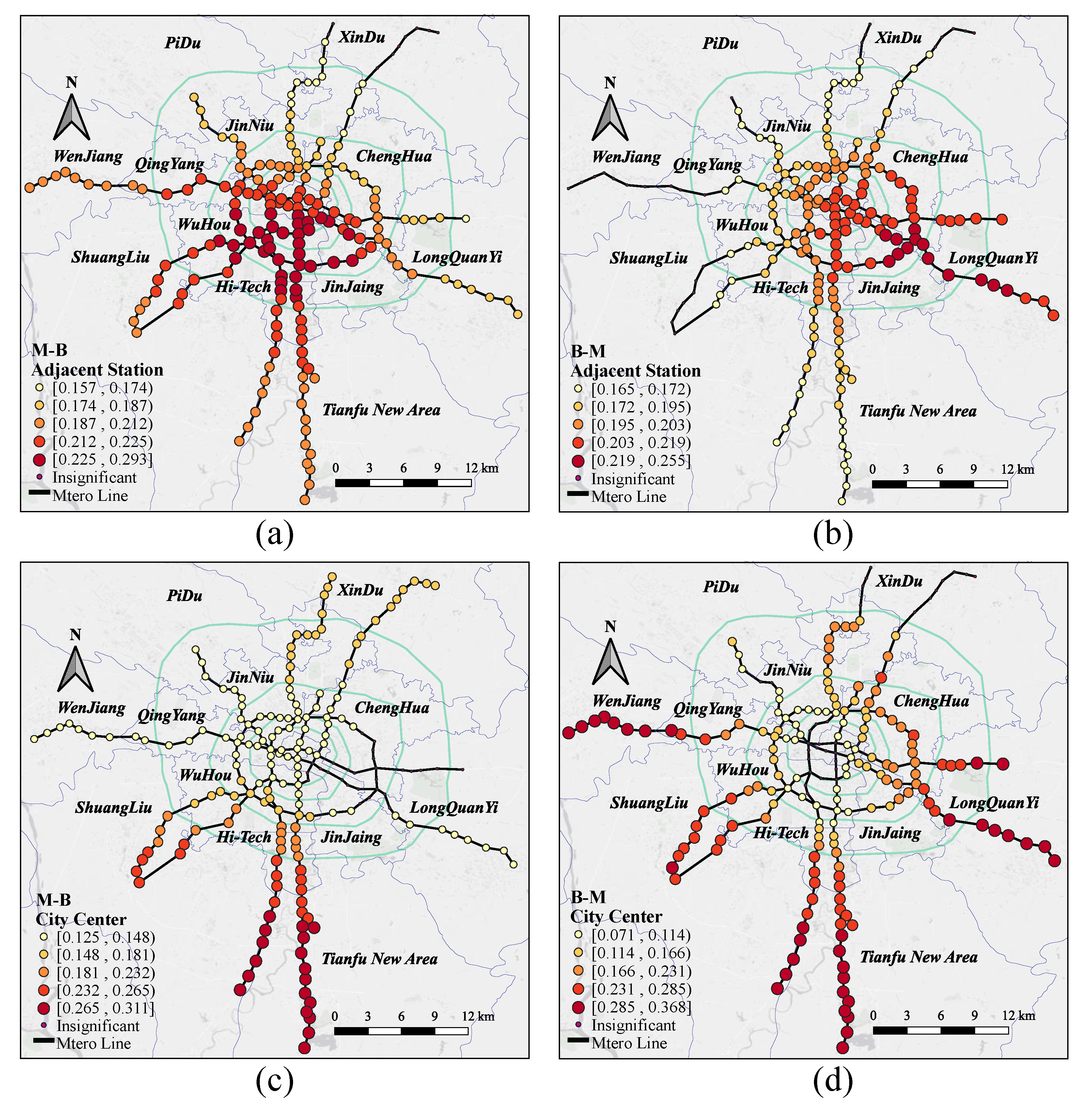
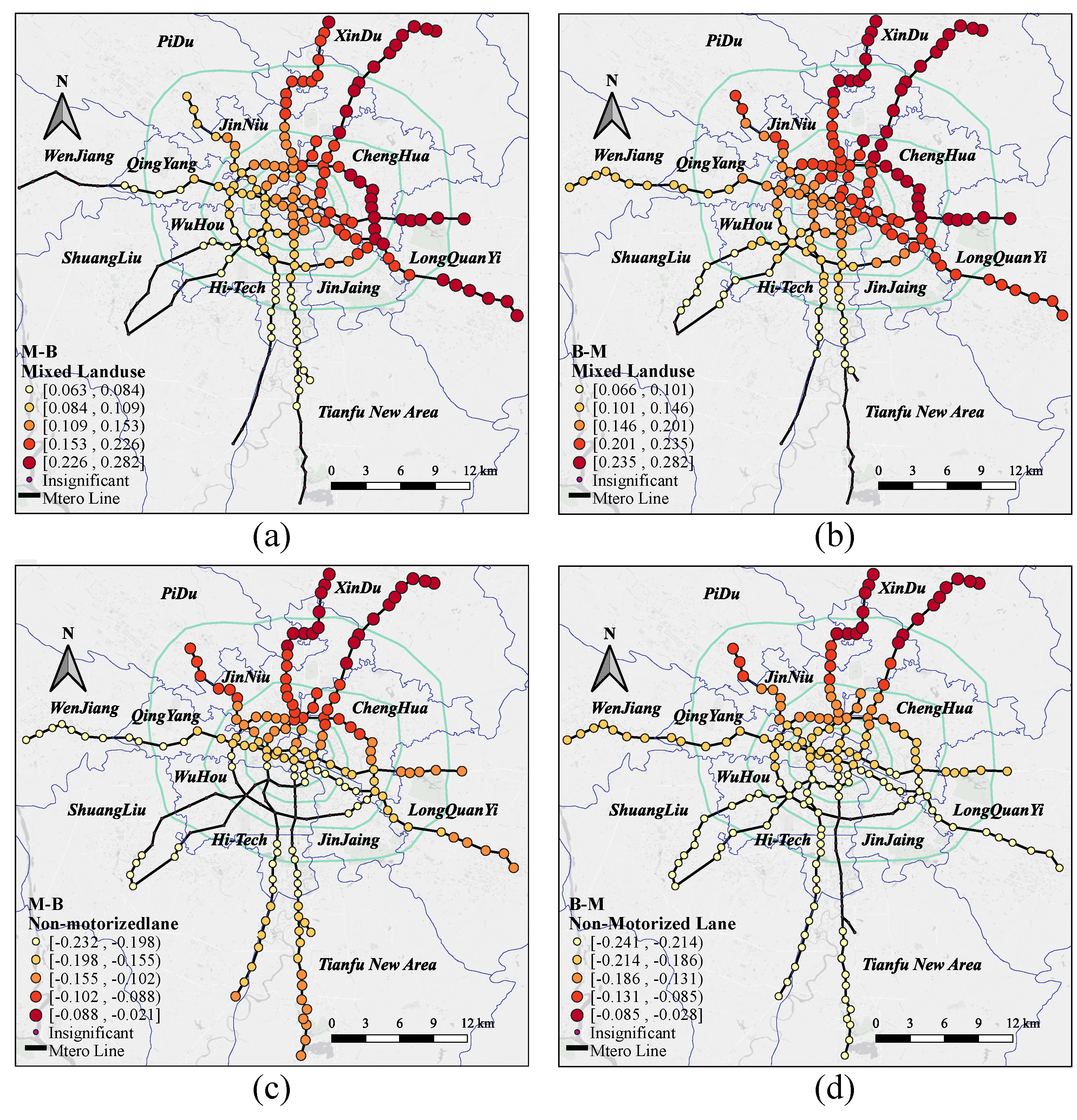
The spatial configuration of metro stations and their built environment, including factors such as distance, design, variety, density, and accessibility, are critical determinants of passenger travel behaviour [60,61]. Since the estimation coefficient of each independent variable varies from station to station, Figure 6, Figure 7, Figure 8 and Figure 9 show metro stations in different colours according to the value of their estimation coefficient, to make it easier to understand the spatial variations in the impact of the independent variables.
The spatially varying effects of the bus system variables on the transfer mode are shown in Figure 7. In terms of coefficient means, Bus Stop and Bus Line have the strongest impact on transfer passengers of all indicators. Figure 7a,b shows the spatial variation in variable Bus Stop on the transfer ridership. Bus Stop is significantly associated with the transfer ridership in the two transfer modes. The average coefficients are 0.368 and 0.373 for the M-B and B-M, respectively. Meanwhile, it can be observed that certain insignificant stations are located in distant suburban regions, such as Wenjiang or Tianfu New Area. Furthermore, they have higher coefficients inside the ring road than their counterparts outside, and both show a multi-layered distribution pattern characterized by a radial decrease from the city centre to the suburbs. The results of the study show that a higher distribution of bus stops around metro stations in Ring 3 can attract a large number of passengers and effectively improve the transfer of passengers.
Figure 7c,d shows the influence of the spatially varying variable Bus Line on the transfer ridership. The figures show that the Bus Line is positively correlated with the transfer ridership. The average coefficients are 0.455 and 0.401 for the M-B and B-M, respectively. After comparing the coefficients of Bus Stop with Bus Line for B-M and M-B, it is found that Bus Line is better than Bus Stop in promoting transfer ridership. This result may be since the more bus lines that pass through a metro station, the better the accessibility of the destination. Therefore, increasing the number of bus stops in the catchment area of a metro station is the most effective way to increase the number of passengers transferring between bus and metro.
As shown in Figure 8, Metro Line and Station Accessibility represent the extent to which the structural characteristics of the metro network affect the M-B and B-M transfer ridership. Figure 8a,b shows the influence of the spatially varying variable Metro Line on the transfer ridership. The figures show that the Metro Line is positively correlated with transfer ridership. The average coefficients are 0.267 and 0.272 for the M-B and B-M, respectively. The increase in Metro Line will attract more passengers from different destinations, thus contributing to the flow of transfer ridership between metro and bus. In terms of the spatial distribution of the Metro Line coefficient, the M-B model mainly affects the northern area of Metro Line 3 and Metro Line 7 in the east-west direction, while the B-M model mainly affects the southwest area from Tianfu Square to the 4th Ring Road, with some spatial variability.
Figure 8c,d shows the influence of the spatially varying variable Station Accessibility on the transfer ridership. The average coefficients are 0.278 and 0.285 for the M-B and B-M, respectively. From the spatial distribution of the coefficients in the figure, the impact of Station Accessibility on both transfer modes is similar in terms of degree and distribution area. The areas with the greatest impact on Station Accessibility are concentrated in the city centre and the northern part of the city. One possible explanation is that the high level of metro accessibility in the northern part of Chengdu indicates a long distance from metro stations in the region to other metro stations in the metro network. During workdays, long-distance travel necessitates transfer between bus and metro systems.
As shown in Figure 9, Adjacent station and City Center show the impact of the urban design dimension on M-B and B-M transfer ridership. Figure 9a,b shows the influence of the spatially varying variable Adjacent station on the transfer ridership. The average coefficients are 0.235 and 0.228 for the M-B and B-M, respectively. Based on the spatial distribution of the coefficients of Adjacent station, a gradual decrease of the coefficient from the center to the periphery is observed for both transfer modes. Specifically, M-B shows a slower decrease towards the south and a faster decrease towards the north, while B-M shows a slower decrease towards the east. The positive facilitation effect of Adjacent station could be attributed to the fact that an increase in the distance between adjacent metro stations encourages passengers to use public transport to reach the metro station.
Figure 9c,d shows the influence of the spatially varying variable City Center on the transfer ridership. The average coefficients are 0.212 and 0.203 for the M-B and B-M, respectively. The figure shows that the effect of the variable City Center is more pronounced in suburban stations. This can be attributed to the sparser metro network and fewer bus routes in suburban areas, which results in limited direct access to destinations and motivates passengers to transfer between bus and metro for medium- and long-distance trips.
As shown in Figure 10, Mixed land use and Non-motorized lane show the impact of the level of development around the station on M-B and B-M transfer ridership. Figure 10a,b shows the influence of the spatially varying variable Mixed land use on the transfer ridership. The average coefficients are 0.176 and 0.178 for the M-B and B-M, respectively. Despite the greater sensitivity of the M-B transfer mode to Mixed land use, the overall impact on both transfer modes is limited. Furthermore, the regional heterogeneity of impact intensity shows a similar pattern, gradually increasing from the city centre to the north-east region, which is characterised by diverse land use patterns, higher Mixed land use values and stable weekday transfer demand.
Figure 10c,b shows the influence of the spatially varying variable Non-motorized lane on the transfer ridership. The average coefficients of −0.122 and −0.131 for M-B and B-M, respectively, exhibit a significant negative effect. The negative impact could be attributed to the rising non-motorized density in the vicinity of the stations, which encourages commuters to opt for alternative modes such as bike-sharing and subsequently reduces the likelihood of choosing B-M or M-B for transfer purposes.
The analysis of variables Mixed land use and Non-motorized lane showed that the level of station development had a relatively small effect on B-M and M-B transfer ridership compared to other indicators. This outcome implies that altering the level of development surrounding a metro station has a limited impact on both B-M and M-B transfer ridership between metro and bus.

5. Conclusions

Gaining insight into the passengers of diverse transportation modes constitutes a valuable pursuit towards realizing a sustainable and low-carbon urban transportation system. Nevertheless, the exploration of spatial disparities in transfer passengers between bus and metro systems, as well as the identification of the factors that influence them, remains an area of limited research efforts. This study aims to address the knowledge gaps in the existing literature by utilizing the empirical analysis to examine the spatial heterogeneity of transfer ridership in metro and bus systems, as well as their interrelationships with various variables, in the context of Chengdu, China. The major findings can be summarized as follows:
(1)
Compared to OLS and GWR models, the MGWR model has demonstrated superior effectiveness in accounting for spatial heterogeneity at different scales. The inclusion of scale effects for built environment variables in the MGWR model allows for more precise local parameter estimates and more reliable estimation results, particularly for bus and metro transfer modes. The results show that the MGWR model outperforms the GWR model by 8.6% and 5.77% for the Adj.R2 for B-M and M-B transfer modes, respectively. In addition, the magnitude of the influence of built environment variables on metro and bus transfer modes is better represented by a 13.34% reduction in parameter AICc. This finding provides further evidence of the spatial heterogeneity of built environment variables and their influence on metro and bus transfer modes.
(2)
The spatial scale heterogeneity of built environment factors across different dimensions has a significant impact on metro and bus transfer modes. The results of the MGWR optimal bandwidth analysis show that the number of bus routes has the smallest scale of effect on both M-B and B-M modes while exhibiting the most significant spatial heterogeneity. In comparison, land use mix and non-highway density show a similar scale of effect to the global scale, with relatively less spatial heterogeneity.
(3)
The impact of the different variables differs between the M-B and B-M modes. The results show that the variables Bus Stop and Bus Line have a greater impact, while the variables Mixed land use and Non-motorized lane have the least impact, with variable Non-motorized lane having a significant negative impact. These results suggest that increasing the number of bus stops and lines around a metro station is the most effective way to increase metro and bus transfer passengers. Increasing the number of bus lines around the station is more effective than increasing the number of bus stops.
Empirical findings for Chengdu reveal significant regional differences in the impact of the built environment on B-M and M-B transfer ridership. As such, optimizing the built environment for different regional stations proves necessary to enhance the residents’ travel structure and promote the coordinated development of public transport systems.
There are several limitations to this study that need to be acknowledged. Firstly, the lack of data on population density and regional economy meant that these variables were omitted from the model, potentially biasing the results. Secondly, the buffer selection method used to identify the catchment areas of metro stations involved a circular buffer zone with a radius of 800 m and Tyson polygons were used. This approach may have introduced some bias, particularly in the city center where many stations are concentrated, and their catchment areas are smaller. Despite some limitations, this study provides a systematic exploration of the spatial variation patterns of metro and bus transfer ridership and examines the impact of the built environment on their spatial heterogeneity. Meanwhile, it is worth noting that the MGWR model used in this study is limited to capturing only the spatially varying relationship between the explanatory variables and the response variable and does not consider the temporal dimension of the data.

Author Contributions

Conceptualization, X.L.; Data curation, X.L.; Formal analysis, Y.M.; Funding acquisition, Y.M. and C.L.; Investigation, X.L.; Methodology, Q.Y.; Project administration, Q.Y.; Software, X.L.; Supervision, Y.M. and C.L. Writing—original draft, X.L. and C.L. All authors have read and agreed to the published version of the manuscript.

Funding

This research was funded by Young Scientists Fund of the National Natural Science Foundation of China (grant No. 52002127), Jiangxi Provincial Youth Project for Humanities and Social Sciences Research in Universities (grant No. GL21201), Education of Humanities and social science research on Youth Fund Project (grant No. 19YJC630121), Sichuan Science and Technology Program (grant No. 2022YFG0197, No.2022JDR0324), Sichuan Social Sciences Program (grant No. SC21C088).

Institutional Review Board Statement

Not applicable.

Informed Consent Statement

Not applicable.

Data Availability Statement

The data presented in this study are available on request from the corresponding author.

Acknowledgments

This research was funded by Young Scientists Fund of the National Natural Science Foundation of China (grant No. 52002127), Jiangxi Provincial Youth Project for Humanities and Social Sciences Research in Universities (grant No. GL21201), Education of Humanities and social science research on Youth Fund Project (grant No. 19YJC630121), Sichuan Science and Technology Program (grant No. 2022YFG0197, No.2022JDR0324). This work was supported by Young Scientists Fund of the National Natural Science Foundation of Chine, Jiangxi Provincial Youth Project for Humanities and Social Sciences Research in University, Education of Humanities and social science research on Youth Fund Project and Sichuan Science and Technology Program.

Conflicts of Interest

The authors declare no conflict of interest.

References

  1. Wu, P.; Xu, L.; Li, J.; Guo, H.; Huang, Z. Recognizing Real-Time Transfer Patterns between Metro and Bus Systems Based on Spatial–Temporal Constraints. J. Transp. Eng. Part A Syst. 2022, 148, 04022065. [Google Scholar] [CrossRef]
  2. Wang, D.; Zhou, M. The Built Environment and Travel Behavior in Urban China: A Literature Review. Transp. Res. Part D Transp. Environ. 2017, 52, 574–585. [Google Scholar] [CrossRef]
  3. Jiang, S.; Guan, W.; He, Z.; Yang, L. Exploring the Intermodal Relationship between Taxi and Subway in Beijing, China. J. Adv. Transp. 2018, 2018, 3981845. [Google Scholar] [CrossRef]
  4. Li, P.; Lu, Y.; Wang, J. The Effects of Fuel Standards on Air Pollution: Evidence from China. J. Dev. Econ. 2020, 146, 102488. [Google Scholar] [CrossRef]
  5. Wei, H. Impacts of China’s National Vehicle Fuel Standards and Subway Development on Air Pollution. J. Clean. Prod. 2019, 241, 118399. [Google Scholar] [CrossRef]
  6. Lin, D.; De Vos, J.; Maruyama, T.; Bobylev, N.; Cui, J. Metro-Related Transfers: A Review of Recent Literature. J. Urban Plan. Dev. 2022, 148, 03122002. [Google Scholar] [CrossRef]
  7. Seaborn, C.; Attanucci, J.; Wilson, N. Analyzing Multimodal Public Transport Journeys in London with Smart Card Fare Payment Data. Transp. Res. Rec. J. Transp. Res. Board 2009, 2121, 55–62. [Google Scholar] [CrossRef]
  8. Huang, Z.; Xu, L.; Lin, Y.; Wu, P.; Feng, B. Citywide Metro-to-Bus Transfer Behavior Identification Based on Combined Data from Smart Cards and GPS. Appl. Sci. 2019, 9, 3597. [Google Scholar] [CrossRef]
  9. Schakenbos, R.; Paix, L.L.; Nijenstein, S.; Geurs, K.T. Valuation of a Transfer in a Multimodal Public Transport Trip. Transp. Policy 2016, 46, 72–81. [Google Scholar] [CrossRef]
  10. Crane, R.; Scweitzer, L.A. Transport and Sustainability: The Role of the Built Environment. Built Environ. 2003, 29, 238–252. [Google Scholar] [CrossRef]
  11. Yu, L.; Xie, B.; Chan, E. How Does the Built Environment Influence Public Transit Choice in Urban Villages in China? Sustainability 2018, 11, 148. [Google Scholar] [CrossRef]
  12. Zhang, Y.; Thomas, T.; Brussel, M.; van Maarseveen, M. Exploring the Impact of Built Environment Factors on the Use of Public Bikes at Bike Stations: Case Study in Zhongshan, China. J. Transp. Geogr. 2017, 58, 59–70. [Google Scholar] [CrossRef]
  13. Van Acker, V.; Derudder, B.; Witlox, F. Why People Use Their Cars While the Built Environment Imposes Cycling. JTLU 2013, 6, 53–62. [Google Scholar] [CrossRef]
  14. Titze, S.; Stronegger, W.J.; Janschitz, S.; Oja, P. Association of Built-Environment, Social-Environment and Personal Factors with Bicycling as a Mode of Transportation among Austrian City Dwellers. Prev. Med. 2008, 47, 252–259. [Google Scholar] [CrossRef]
  15. Wey, W.-M.; Zhang, H.; Chang, Y.-J. Alternative Transit-Oriented Development Evaluation in Sustainable Built Environment Planning. Habitat Int. 2016, 55, 109–123. [Google Scholar] [CrossRef]
  16. Kamruzzaman, M.D.; Baker, D.; Washington, S.; Turrell, G. Advance Transit Oriented Development Typology: Case Study in Brisbane, Australia. J. Transp. Geogr. 2014, 34, 54–70. [Google Scholar] [CrossRef]
  17. Renne, J.L. From Transit-Adjacent to Transit-Oriented Development. Local Environ. 2009, 14, 1–15. [Google Scholar] [CrossRef]
  18. Cherry, T.; Townsend, C. Assessment of Potential Improvements to Metro–Bus Transfers in Bangkok, Thailand. Transp. Res. Rec. J. Transp. Res. Board 2012, 2276, 116–122. [Google Scholar] [CrossRef]
  19. Nesheli, M.M.; Ceder, A. (Avi) Improved Reliability of Public Transportation Using Real-Time Transfer Synchronization. Transp. Res. Part C Emerg. Technol. 2015, 60, 525–539. [Google Scholar] [CrossRef]
  20. Munizaga, M.A.; Carolina, P. Estimation of a Disaggregate Multimodal Public Transport Origin–Destination Matrix from Passive Smartcard Data from Santiago, Chile. Transp. Res. Part C Emerg. Technol. 2012, 24, 9–18. [Google Scholar] [CrossRef]
  21. Munizaga, M.A.; Gschwender, A.; Gallegos, N. Fare Evasion Correction for Smartcard-Based Origin-Destination Matrices. Transp. Res. Part A Policy Pract. 2020, 141, 307–322. [Google Scholar] [CrossRef]
  22. Sun, Y.; Shi, J.; Schonfeld, P.M. Identifying Passenger Flow Characteristics and Evaluating Travel Time Reliability by Visualizing AFC Data: A Case Study of Shanghai Metro. Public Transp. 2016, 8, 341–363. [Google Scholar] [CrossRef]
  23. Zhao, J.; Qu, Q.; Zhang, F.; Xu, C.; Liu, S. Spatio-Temporal Analysis of Passenger Travel Patterns in Massive Smart Card Data. IEEE Trans. Intell. Transport. Syst. 2017, 18, 3135–3146. [Google Scholar] [CrossRef]
  24. Zhao, D.; Wang, W.; Woodburn, A.; Ryerson, M.S. Isolating High-Priority Metro and Feeder Bus Transfers Using Smart Card Data. Transportation 2017, 44, 1535–1554. [Google Scholar] [CrossRef]
  25. Arbab, P.; Martinez, J.; Amer, S.; Pfeffer, K. Toward Active Transport as a Utilitarian and Recreational Form of Sustainable Urban Mobility. In Advances in Mobility-as-a-Service Systems, Proceedings of the 5th Conference on Sustainable Urban Mobility, Virtual CSUM2020, Volos, Greece, 17–19 June 2020; Nathanail, E.G., Adamos, G., Karakikes, I., Eds.; Springer International Publishing: Cham, Switzerland, 2021; pp. 635–644. [Google Scholar]
  26. Ewing, R.; Cervero, R. Travel and the Built Environment: A Meta-Analysis. J. Am. Plan. Assoc. 2010, 76, 265–294. [Google Scholar] [CrossRef]
  27. Cervero, R.; Kockelman, K. Travel Demand and the 3Ds: Density, Diversity, and Design. Transp. Res. Part D Transp. Environ. 1997, 2, 199–219. [Google Scholar] [CrossRef]
  28. Yu, L.; Xie, B.; Chan, E.H.W. Exploring Impacts of the Built Environment on Transit Travel: Distance, Time and Mode Choice, for Urban Villages in Shenzhen, China. Transp. Res. Part E Logist. Transp. Rev. 2019, 132, 57–71. [Google Scholar] [CrossRef]
  29. Wang, X.; Shao, C.; Yin, C.; Dong, C. Exploring the Effects of the Built Environment on Commuting Mode Choice in Neighborhoods near Public Transit Stations: Evidence from China. Transp. Plan. Technol. 2021, 44, 111–127. [Google Scholar] [CrossRef]
  30. Gao, K.; Yang, Y.; Sun, L.; Qu, X. Revealing Psychological Inertia in Mode Shift Behavior and Its Quantitative Influences on Commuting Trips. Transp. Res. Part F Traffic Psychol. Behav. 2020, 71, 272–287. [Google Scholar] [CrossRef]
  31. Pan, H.; Li, J.; Shen, Q.; Shi, C. What Determines Rail Transit Passenger Volume? Implications for Transit Oriented Development Planning. Transp. Res. Part D Transp. Environ. 2017, 57, 52–63. [Google Scholar] [CrossRef]
  32. Zhao, J.; Deng, W.; Song, Y.; Zhu, Y. Analysis of Metro Ridership at Station Level and Station-to-Station Level in Nanjing: An Approach Based on Direct Demand Models. Transportation 2014, 41, 133–155. [Google Scholar] [CrossRef]
  33. Liu, D.; Rong, W.; Zhang, J.; Ge, Y.-E. (Ethan) Exploring the Nonlinear Effects of Built Environment on Bus-Transfer Ridership: Take Shanghai as an Example. Appl. Sci. 2022, 12, 5755. [Google Scholar] [CrossRef]
  34. An, R.; Wu, Z.; Tong, Z.; Qin, S.; Zhu, Y.; Liu, Y. How the Built Environment Promotes Public Transportation in Wuhan: A Multiscale Geographically Weighted Regression Analysis. Travel Behav. Soc. 2022, 29, 186–199. [Google Scholar] [CrossRef]
  35. Mainali, J.; Chang, H.; Chun, Y. A Review of Spatial Statistical Approaches to Modeling Water Quality. Prog. Phys. Geogr. Earth Environ. 2019, 43, 801–826. [Google Scholar] [CrossRef]
  36. Zhu, P.; Ho, S.N.; Jiang, Y.; Tan, X. Built Environment, Commuting Behaviour and Job Accessibility in a Rail-Based Dense Urban Context. Transp. Res. Part D Transp. Environ. 2020, 87, 102438. [Google Scholar] [CrossRef]
  37. Fotheringham, A.S.; Charlton, M.E.; Brunsdon, C. Geographically Weighted Regression: A Natural Evolution of the Expansion Method for Spatial Data Analysis. Environ. Plan A 1998, 30, 1905–1927. [Google Scholar] [CrossRef]
  38. Li, S.; Lyu, D.; Huang, G.; Zhang, X.; Gao, F.; Chen, Y.; Liu, X. Spatially Varying Impacts of Built Environment Factors on Rail Transit Ridership at Station Level: A Case Study in Guangzhou, China. J. Transp. Geogr. 2020, 82, 102631. [Google Scholar] [CrossRef]
  39. Fotheringham, A.S.; Yang, W.; Kang, W. Multiscale Geographically Weighted Regression (MGWR). Ann. Am. Assoc. Geogr. 2017, 107, 1247–1265. [Google Scholar] [CrossRef]
  40. Iyanda, A.E.; Osayomi, T. Is There a Relationship between Economic Indicators and Road Fatalities in Texas? A Multiscale Geographically Weighted Regression Analysis. GeoJournal 2021, 86, 2787–2807. [Google Scholar] [CrossRef]
  41. Chen, E.; Ye, Z.; Wang, C.; Zhang, W. Discovering the Spatio-Temporal Impacts of Built Environment on Metro Ridership Using Smart Card Data. Cities 2019, 95, 102359. [Google Scholar] [CrossRef]
  42. Kumar, P.; Khani, A.; He, Q. A Robust Method for Estimating Transit Passenger Trajectories Using Automated Data. Transp. Res. Part C Emerg. Technol. 2018, 95, 731–747. [Google Scholar] [CrossRef]
  43. Yang, H.; Li, X.; Li, C.; Huo, J.; Liu, Y. How Do Different Treatments of Catchment Area Affect the Station Level Demand Modeling of Urban Rail Transit? J. Adv. Transp. 2021, 2021, 2763304. [Google Scholar] [CrossRef]
  44. Jin, M.; Wang, M.; Gong, Y.; Liu, Y. Spatio-Temporal Constrained Origin-Destination Inferring Using Public Transit Fare Card Data. Phys. A Stat. Mech. Its Appl. 2022, 127642. [Google Scholar] [CrossRef]
  45. Gade, K. A Non-Singular Horizontal Position Representation. J. Navig. 2010, 63, 395–417. [Google Scholar] [CrossRef]
  46. Limpert, E.; Stahel, W.A.; Abbt, M. Log-Normal Distributions across the Sciences: Keys and Clues. BioScience 2001, 51, 341. [Google Scholar] [CrossRef]
  47. Wu, P.; Xu, L.; Zhong, L.; Gao, K.; Qu, X.; Pei, M. Revealing the Determinants of the Intermodal Transfer Ratio between Metro and Bus Systems Considering Spatial Variations. J. Transp. Geogr. 2022, 104, 103415. [Google Scholar] [CrossRef]
  48. Wang, C.; Qiu, Z.; Pan, R.; Wang, X.; Yan, Y. Exploring the Spatial Variation of Access/Egress Distances of Subway Stations Using Mobile Phone Positioning Data in Chengdu, China. J. Adv. Transp. 2023, 2023, e8008667. [Google Scholar] [CrossRef]
  49. Tao, T.; Wang, J.; Cao, X. Exploring the Non-Linear Associations between Spatial Attributes and Walking Distance to Transit. J. Transp. Geogr. 2020, 82, 102560. [Google Scholar] [CrossRef]
  50. El-Geneidy, A.; Grimsrud, M.; Wasfi, R.; Tétreault, P.; Surprenant-Legault, J. New Evidence on Walking Distances to Transit Stops: Identifying Redundancies and Gaps Using Variable Service Areas. Transportation 2014, 41, 193–210. [Google Scholar] [CrossRef]
  51. Wu, P.; Li, J.; Pian, Y.; Li, X.; Huang, Z.; Xu, L.; Li, G.; Li, R. How Determinants Affect Transfer Ridership between Metro and Bus Systems: A Multivariate Generalized Poisson Regression Analysis Method. Sustainability 2022, 14, 9666. [Google Scholar] [CrossRef]
  52. Bao, Z.; Lu, W. Applicability of the Environmental Kuznets Curve to Construction Waste Management: A Panel Analysis of 27 European Economies. Resour. Conserv. Recycl. 2023, 188, 106667. [Google Scholar] [CrossRef]
  53. Anselin, L.; Arribas-Bel, D. Spatial Fixed Effects and Spatial Dependence in a Single Cross-Section: Spatial Fixed Effects and Spatial Dependence. Pap. Reg. Sci. 2013, 92, 3–17. [Google Scholar] [CrossRef]
  54. Brunsdon, C.; Fotheringham, A.S.; Charlton, M.E. Geographically Weighted Regression: A Method for Exploring Spatial Nonstationarity. Geogr. Anal. 2010, 28, 281–298. [Google Scholar] [CrossRef]
  55. Liao, F.; Tian, Q.; Arentze, T.; Huang, H.-J.; Timmermans, H.J.P. Travel Preferences of Multimodal Transport Systems in Emerging Markets: The Case of Beijing. Transp. Res. Part A Policy Pract. 2020, 138, 250–266. [Google Scholar] [CrossRef]
  56. Hernandez, S.; Monzon, A. Key Factors for Defining an Efficient Urban Transport Interchange: Users’ Perceptions. Cities 2016, 50, 158–167. [Google Scholar] [CrossRef]
  57. Mollalo, A.; Vahedi, B.; Rivera, K.M. GIS-Based Spatial Modeling of COVID-19 Incidence Rate in the Continental United States. Sci. Total Environ. 2020, 728, 138884. [Google Scholar] [CrossRef] [PubMed]
  58. Oshan, T.M.; Smith, J.; Fotheringham, A.S. Targeting the Spatial Context of Obesity Determinants via Multiscale Geographically Weighted Regression; Open Science Framework: Charlottesville, VA, USA, 2020. [Google Scholar]
  59. Wang, S.; Noland, R.B. Variation in Ride-Hailing Trips in Chengdu, China. Transp. Res. Part D Transp. Environ. 2021, 90, 102596. [Google Scholar] [CrossRef]
  60. Liu, J.; Chau, K.W.; Bao, Z. Multiscale Spatial Analysis of Metro Usage and Its Determinants for Sustainable Urban Development in Shenzhen, China. Tunn. Undergr. Space Technol. 2023, 133, 104912. [Google Scholar] [CrossRef]
  61. Manville, M. Travel and the Built Environment: Time for Change. J. Am. Plan. Assoc. 2017, 83, 29–32. [Google Scholar] [CrossRef]
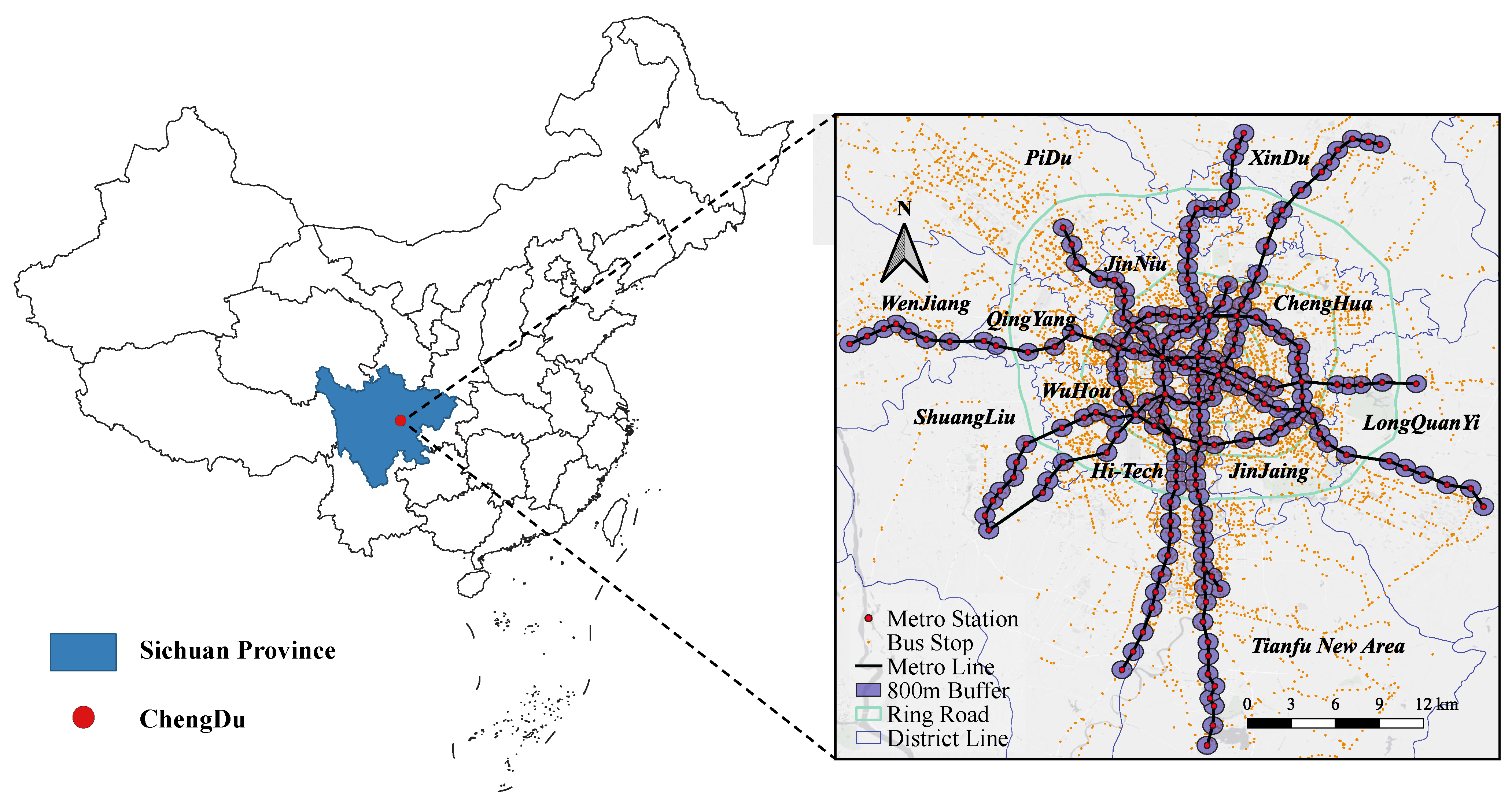
Figure 1. Study area and buffer zone of the metro station.
Sustainability 15 07891 g001
Figure 2. Daily passengers on the metro and bus systems.
Sustainability 15 07891 g002
Figure 3. Workflow of transfer identification.
Sustainability 15 07891 g003
Figure 4. Inferred bus vehicle’s arrival and departure times.
Sustainability 15 07891 g004
Figure 5. Transfer ridership of bus-to-metro and metro-to-bus on weekdays.
Sustainability 15 07891 g005
Figure 6. Spatial distribution of transfer ridership: (a) the transfer ridership of the M-B mode, (b) the transfer ridership of the B-M mode.
Sustainability 15 07891 g006
Figure 7. Spatial distribution of the coefficients of variables Bus Stop and Bus Line in the MGWR model: (a,b) Effects of Bus Stop on the M-B and B-M, respectively; (c,d) Effects of Bus Line on the M-B and B-M, respectively.
Sustainability 15 07891 g007
Figure 8. Spatial distribution of the coefficients of variables Metro Line, Station Accessibility in the MGWR model: (a,b) Effects of Metro Line on the M-B and B-M, respectively; (c,d) Effects of Station Accessibility on the M-B and B-M, respectively.
Sustainability 15 07891 g008
Figure 9. Spatial distribution of the coefficients of variables Adjacent station and City Center in the MGWR model: (a,b) Effects of Adjacent station on the M-B and B-M, respectively; (c,d) Effects of City Center on the M-B and B-M, respectively.
Sustainability 15 07891 g009
Figure 10. Spatial distribution of the coefficients of variables Mixed land use and Non-motorized lane in the MGWR model: (a,b) Effects of Mixed land use on the M-B and B-M, respectively; (c,d) Effects of Non-motorized lane on the M-B and B-M, respectively.
Sustainability 15 07891 g010
Table 1. Descriptive statistics of the explanatory variables.
VariablesDescriptionMeanS.DSource
Bus StopThe number of bus stops21.4013.20Chengdu Public Transport Group
Bus LineThe number of bus lines passing through21.9817.64Chengdu Public Transport Group
Station
Accessibility
The distance to other stations on the metro network14.153.79Chengdu Rail Transit Group
Metro LineThe number of metro lines passing through1.240.49ArcGIS
TerminalIs it a terminal station? 1 means yes, 0 means no0.070.25ArcGIS
Adjacent
station
The average distance to adjacent metro stations1.550.54ArcGIS
City CenterThe straight line distance from the city center10.396.64ArcGIS
Non-motorized laneThe density of the non-motorized lane12.845.11Amap
Mixed land useThe Shannon entropy of POI categories0.630.10Amap
Table 2. Inference of vehicle arrival and boarding for different lines.
Bus LinesBus Vehicle Arrivals
at Morning or Evening Peak
Morning or Evening Peak Boarding Passengers
Time IntervalMaximum Error Number of StopsTotal Number of Error StopsReal
Passengers
Inferred
Passengers
Error
4914.45 s1814.7814.36−2.84
5618.64 s 1429.0829.631.89
7313.25 s0513.8514.132.02
Table 3. The results of the multicollinearity test and spatial autocorrelation test.
VariablesMulticollinearity Spatial Autocorrelation
VIFM-BVIFB-MMoran’s IZ-Valuep-Value
YM-B0.47412.247<0.001
YB-M0.40910.574<0.001
Bus Stop3.343.290.44513.309<0.001
Bus Line3.33.30.3649.735<0.001
Metro Line4.374.340.4137.269<0.001
Station Accessibility1.281.280.4347.583<0.001
Terminal1.171.190.3616.508<0.001
Adjacent station1.631.510.4998.816<0.001
City Center4.154.20.39910.361<0.001
Non-motorized lane2.342.180.43111.175<0.001
Mixed land use1.161.120.0772.161<0.001
Table 4. Results of the OLS model.
VariablesM-B_OLSB-M_OLS
CoefficientT-Valuep-ValueVIFCoefficientT-Valuep-ValueVIF
Intercept6.34719.6520.0429.24524.9880.033
Bus Stop0.184 *5.684 0.0223.340.153 *8.097 0.0153.29
Bus Line0.237 *5.891 0.0153.300.211 *3.426 0.0183.30
Metro Line0.151 *4.836 0.0174.370.128 *6.135 0.0354.34
Station Accessibility0.222 **4.003 0.0041.280.149 *4.967 0.0291.28
Terminal0.094 *6.810 0.0151.170.114 *7.358 0.0111.19
Adjacent station0.145 *3.177 0.0331.630.201 *5.245 0.0321.51
City Center0.164 *5.160 0.0144.150.178 **2.382 0.0064.20
Non-motorized lane−0.088 **−2.272 0.0022.34−0.091 **−4.663 0.0032.18
Mixed land use0.155 *4.609 0.0311.160.199 *2.504 0.0231.12
Note: * indicates a significance of 0.05; ** indicates significance of 0.01.
Table 5. Results of the GWR and MGWR models.
VariablesM-B_GWRM-B_MGWRB-M_GWRB-M_MGWR
MeanS.DMeanS.DMeanS.DMeanS.D
Bus Stop0.221 *0.017 0.373 **0.017 0.240 *0.015 0.368 **0.017
Bus Line0.276 *0.014 0.455 *0.018 0.297 *0.020 0.401 *0.013
Metro Line0.203 *0.006 0.272 *0.008 0.183 *0.017 0.267 *0.014
Station Accessibility0.213 *0.010 0.285 **0.005 0.148 *0.003 0.278 **0.014
Terminal0.155 *0.003 0.227 *0.002 0.184 *0.011 0.203 *0.020
Adjacent station0.193 *0.003 0.228 *0.002 0.216 *0.012 0.235 *0.009
City Center0.217 *0.008 0.203 *0.003 0.164 **0.015 0.212 **0.005
Non-motorized lane−0.127 **0.006 −0.131 **0.013 −0.133 **0.020 -0.122 **0.012
Mixed land use0.211 *0.018 0.178 *0.002 0.238 *0.014 0.176 *0.015
Note: 1. Coefficients are normalized; 2. The MGWR and GWR models are local regression models, generating coefficients as the mean of each local coefficient; 3. * indicates a significance of 0.05; ** indicates significance of 0.01.
Table 6. Comparison of the goodness of fit measures for the global and local models.
AICcRSSR2Adj.R2
M-B_OLS539.895164.1290.1930.146
M-B_GWR382.102114.3320.7820.741
M-B_MGWR322.85639.5320.7990.754
B-M_OLS539.321163.6410.2350.192
B-M_GWR359.16471.5780.7880.77
B-M_MGWR311.2533.9670.8110.783
Table 7. Optimal bandwidths of the GWR and MGWR models.
BandwidthB-MM-B
MGWRGWRMGWRGWR
Bus Stop87799679
Bus Line47793879
Metro Line1297913479
Station Accessibility1567915679
Terminal84799279
Adjacent station68797579
City Center93799379
Non-motorized lane1387913879
Mixed land use1447914479
Disclaimer/Publisher’s Note: The statements, opinions and data contained in all publications are solely those of the individual author(s) and contributor(s) and not of MDPI and/or the editor(s). MDPI and/or the editor(s) disclaim responsibility for any injury to people or property resulting from any ideas, methods, instructions or products referred to in the content.