Article

Assessing Environmental Sustainability Based on the Three-Dimensional Emergy Ecological Footprint (3D EEF) Model: A Case Study of Gansu Province, China

School of Mathematics and Computer Science, Northwest Minzu University, Lanzhou 730030, China
*
Author to whom correspondence should be addressed.
Sustainability 2023, 15(10), 8007; https://doi.org/10.3390/su15108007
Submission received: 4 April 2023 / Revised: 8 May 2023 / Accepted: 11 May 2023 / Published: 14 May 2023

Abstract

:
Quantifying the supply and demand relationship between human social consumption and natural ecosystem resources is an effective way to assess the sustainability of ecosystem services. This paper introduces the concepts of footprint size (EFsize) and depth (EFdepth) to emergy analysis to establish a three-dimensional emergy ecological footprint (3D EEF) model and evaluates the environmental sustainability development of Gansu Province from 2001 to 2020. The results show that the minimum value of the 3D emergy ecological footprint (EEF3D) of Gansu Province was 5.98 × 10⁷ hm2 and that the maximum value was 1.41 × 10⁸ hm2. The EEFdepth was slightly more than one in 2015 and 2016, and the ecological resources were in deficit. However, the ecological service system from 2001 to 2020 was almost in a sustainable state. The region’s emergy carrying capacity (ECC) and emergy ecological footprint (EEF) from 2021 to 2030 are predicted using the ARIMA and GM (1, 1) models. The projections show that the ECC and EEF will increase year by year from 2021 to 2030. In the short term, the flow of natural capital can satisfy the development requirements. Finally, policy recommendations are provided for the ecological sustainability of the region.

1. Introduction

Ecosystems are the foundation for human life and development, providing water, food, and material resources that are essential for human survival. However, with the growth of the population, economic activities, and the improvement of science and technology, the relationship between humans and nature is different from that of the past. Human behavior (the irrational utilization of environmental resources, the fast progress of agriculture and industry, etc.) has a significant impact on ecosystems; therefore, there has been a growing consensus among scholars to quantify the services and values of ecosystems and to promote ecological sustainability [1,2,3]. With the development of industrialization and modernization, the rapid economic development of Gansu Province since 2000; the level of urbanization spiking; the rapid economic growth, to a large extent at the cost of high energy consumption in exchange; and the traditional method of economic growth led Gansu Province to face enormous environmental pressure [1]. How to ensure the rapid and steady development of the economy, population, and society while improving the effective utilization of resources and achieving sustainable development has become the primary problem that needs to be solved. Therefore, proposing a reasonable model to measure the value of the ecological service system can provide an effective method to study the dynamic changes in environmental security in Gansu Province.
Emergy analysis, first proposed by Odum’s team in 1983, is a method used to assess ecosystem services that organically link natural ecosystems to human consumption [4]. Wackernagel and Rees introduced the notion of an ecological footprint (EF) in 1996 in which the EF of any given population (from an entire country or city to a single person) is the area of biological productive land and water dedicated to the production of the natural resources employed and the absorption of the waste produced from the population [5,6]. The public awareness of environmental conservation has been steadily increasing in recent years, and many scholars have devoted themselves to improving EF evaluation methods to enhance the reliability and validity of EF evaluation to furnish a reasonable reference foundation and constructive opinions for facilitating sustainable environmental development. Zhao et al. combined emergy analysis and the EF for the first time to devise a new method of calculating the EF and used the method to assess the ecological service system in Gansu Province [6]. Zhao et al. assessed the environmental sustainability status of a small-scale offshore fishery in the East China Sea using an emergy ecological footprint (EEF) approach [7]. The EEF model translated the production and consumption of different resources into a common unit area, accounting for the level of use of renewable natural resources from an energy perspective [6,8]. Later, Liu et al. applied the EEF theory to assess the ecosystems of the Gannan Tibetan Autonomous Prefecture and made recommendations on how to improve its sustainability [3]. Peng et al. used the improved EEF method to calculate the emergy carrying capacity (ECC) and EEF of the city Qingdao from 2004 to 2014 and to make an evaluation about the safety of its complicated ecosystems [2]. Chen et al. pointed out that the EEF model used the emergy transformity to calculate the ECC with more stable results, and the relationship between human demand and the resource supply of ecosystems from the energy perspective was more representative of the current situation of sustainable development in the region [9]. Mancini’s study summarized the theory related to the carbon footprint in the EF and improved the calculation of one of the key factors, the average forest carbon sink, thus improving the accuracy of the EF [10]. In addition, the application of the EF model was extended to many other aspects [11,12]. However, many scholars found certain limitations in the classical two-dimensional (2D) EF model in the process of studying the model. As mentioned by Yang et al., the 2D EF model does not accurately capture the usage of natural capital [13]. Fang argued that the 2D EF model fails to convey the indisputable role of natural capital stock constancy in supporting ecological stability [14]. Furthermore, Zhang et al. observed that the 2D EF model is limited in its ability to analyze the utilization of land and renewable resources [15].
It was especially important in this setting to establish an ecological footprint accounting system that could quantify the level of natural capital stocks and flows utilized. The three-dimensional EF theory was proposed by Niccolucci et al. in 2009, introducing the concepts of footprint size and depth to elucidate the importance of the flows and stocks of natural capital and taking the reduction or non-decrease in capital stock as the basic criterion for judging whether it is sustainable or not, and the proposal of this model encouraged the vertical development of ecological footprint modeling research [16]. Subsequently, in 2011, it was argued that the 3D EF model, while inheriting the advantages of the traditional EF theory, is able to discriminate between the human consumption of the flows of natural capital and the deployment of stocks [17]. Fang and Reinout brought the 3D EF model to China, examined the method’s research development, and recommended some improvement measures and complementing strategies [18]. Fang et al. were able to improve on the inadequacies of the existing 3D EF model and investigated the spatial and temporal variability of natural capital usage in many locations [14,19,20,21]. Li et al. employed a 3D EF model to calculate Urumqi’s EF and ecological carrying capacity (EC) from 1995 to 2018 [22]. The study by Peng et al. used Beijing as an example and developed a 3D EF model and an “eco-equity-efficiency” framework to assess the sustainability of the ecological resources [23]. Several studies on the degree of human occupation over natural resources and ecological sustainability have been done in recent years, utilizing 2D and 3D EF models to assess the condition of sustainability worldwide [24], nationally [25,26,27], and provincially [28,29,30,31].
In recent years, many scholars have focused on current ecological safety issues as well as predicting future ecological sustainability. Many methods for predicting ecological sustainability include time-series analyses and the gray prediction model. The ARIMA model, proposed by statisticians George Box and Gwilyn Jenkins, is among the most noteworthy models for forecasting time-series data and is commonly available in economic studies [32]. Wang et al. calculated the EC and EF of the Liaohe River Basin from 2001 to 2010 using an EEF model and simulated the dynamics of the EF and EC for 10 years using the ARIMA model [33]. Previously, Zhang et al. employed the ARIMA model to simulate the EF and EC from 1949 to 2009 and predicted the EF changing trend from 2010 to 2015 in Gansu Province [34]. Ma et al. used various forecasting models, such as the ARIMA model, to project energy consumption in South Africa from 2017 to 2030 based on the data from 1998 to 2016 [35]. Wang et al. analyzed the current state of environmental sustainability in China through a freshwater EF and an improved EF and predicted future ecological security using the ARIMA model [27]. Then, the study by Li et al. applied a modified EEF model to assess ecological environmental security in Central Asia over the period of 1992–2014 and used the ARIMA model to project ecological sustainability in these five countries over the period of 2020–2025 [36]. Deng proposed the gray system theory in 1982 [37]. Chen’s study took the Cingjing Region of Taiwan as the research object and made use of the EEF model to assess the ecological environmental security of the region from 2008 to 2014 and the gray model (GM) to predict the EC from 2015 to 2024 [38]. Liu et al. established a 3D EF model and used the GM (1, 1) model to measure the state of the ecological environment in Gansu Province from 2020 to 2030 and, finally, constructed an ecological risk model to make a reasonable assessment of the risk of loss to the ecosystem in the region [39]. The calculation process is relatively simple and has a high prediction accuracy with small data samples. Therefore, it is used by many scholars for prediction and evaluation, solving many issues in manufacturing, life, and technology.
Therefore, the work in this paper is as follows: (1) We developed a 3D EEF model to quantify the scale of the human appropriation of capital flows and the extent of the human depletion of capital stock, consequently, to judge the sustainable development status of Gansu Province. (2) Considering the limited data in this study and trying to predict the 3D EEF in the short term, the ARIMA and GM (1, 1) models were chosen to present the predicted values from multiple perspectives and aspects to further improve model efficiency. (3) The model is replicable and can also be used to calculate and assess the ecological development of other regions.
This paper is structured as follows: In Section 2, the data information used to assess the sustainable development status of Gansu Province is organized; meanwhile, the 3D EEF model and the ARIMA and GM (1, 1) prediction models are developed. In Section 3, the calculation results of the 3D EEF model for Gansu Province from 2001 to 2020 are shown as well as the ecological surplus or deficit situation. In Section 4, the dynamic evolutionary characteristics of the region’s natural capital over the next ten years are projected and assessed. In Section 5, the accounting and assessment results are discussed, pointing out the feasibility of the model.

2. Materials and Methods

The goal of this paper was to assess the ecological security of the ecosystem in Gansu Province from 2001 to 2020 and to forecast the EEF3D from 2021 to 2030. We developed a 3D EEF model to calculate and analyze the changing trend of ECC, EEF, emergy ecological footprint size (EEFsize), emergy ecological footprint depth (EEFdepth), and EEF3D from 2001 to 2020. At the same time, using Eviews 10.0 and SPSS Statistics 21.0 software, the ARIMA and GM (1, 1) models were applied to predict the increasing and decreasing trends in 3D EEF from 2021 to 2030 and then to evaluate ecological sustainability. Finally, reasonable opinions were provided in the hope of providing a practical reference basis for the construction of an ecological economy.

2.1. Study Area

Gansu Province is located in Northwest China on the upstream of the Yangtze River between 32°11′ N and 42°57′ N, 92°13′ E and 108°46′ E (in Figure 1). Gansu Province is a vast area with complex and diverse landscapes. The terrain is elongated, and it is 1659 km long from east to west and 530 km broad from north to south, occupying 4.72% of the total area of China [39]. Most altitudes are above 1000 m, with the most prominent mountain ranges including the Qilian Mountains and the Liupan Mountains. Gansu Province is abundant in wind and solar emergy reserves, reaching a total of 237 million kilowatts of wind energy [40]. Gansu Province is a multi-ethnic province with a resident population of 25,012,200 in 2020.
Since 2000, the speedy development of population and industry in Gansu Province has contributed to the degradation of grassland, desertification of land, environmental contamination, and other ecological problems in some areas, and people’s over-exploitation and use of natural resources has damaged the ecological environment. Therefore, effective quantification of the resources of the ecosystem can contribute to the rational use and moderate exploitation of natural resources in Gansu Province and, more importantly, to the maintenance of a balance between economic development and ecological protection in the region. In addition, the study of the sustainable development of ecosystems in Gansu Province can also conduce to the development and ecological construction of the Yellow River Basin by offering valuable research and reference grounds.

2.2. Data Source

In this paper, the ecological and economic systems of Gansu Province were studied as the study subject. In accordance with the requirements of this study and the criteria of the Ministry of Land and Resources for the classification of land use status, the land types were classified as agricultural land, woodland, grassland, water area, fuel land, and building land. In order to guarantee the trustworthiness and correctness of the study data, this study used data from the Gansu Statistical Yearbook 2001–2020 [41]. This study calculated the ECC, EEF, and EEF3D by counting the total emergy from 2001 to 2020, which were used as the original series to predict the ECC and EEF from 2021 to 2030 so as to obtain the predicted values of the EEF3D from 2021 to 2030. The simulation and prediction of the ECC and EEF was carried out with the software Eviews 10.0 and SPSS Statistics 21.0. The statistical data sources for the EEF of Gansu Province are shown in Table 1.

2.3. Methods

This section introduces the theories of the 3D EEF, ARIMA, and GM (1, 1) models.

2.3.1. Emergy Analysis Theory

Odum defines “emergy” as putting the different types of energy contributions on the same baseline, i.e., a kind of energy required to generate a flow or to store it in the conversion process [42]. For instance, a flow’s or store’s solar emergy is the amount of solar emergy necessary to generate it, which is measured in solar emjoules (abbreviated as sej). At the same time, Odum considers “transformity” as the direct or indirect generation of a unit of emergy of one type by an amount of energy of another type [42]. Hence, a project’s total emergy can be calculated using the following equation [6]:
emergy = effective   energy × transformity
Emergy analysis is the comparison of all goods and services and economies through some transformation into solar emergy so that the natural resources in ecosystems, ecosystem services, and material production in socio-economic systems can be organically combined and quantified.
A fundamental concept is carrying capacity. If the number of a species population surpasses the carrying capacity of its habitat, one possible outcome is that the resources needed to satisfy the species’ survival are depleted. Another is that the waste produced by the species builds up and thus threatens the species. Either way, the species may disappear. Societal natural resources include renewable and irreducible resources, with irreducible resources such as coal, oil, rare earths, ore resources, etc. [43]. As the carrying capacity of irreducible resources is discontinuous, only renewable resources need to be calculated. Renewable resources include solar radiation energy, wind energy, rain potential energy, chemical energy of rainwater, energy of Earth’s rotation, tidal energy, etc. [7]. They can be classified according to their sources among which (1) solar radiation energy, wind energy, rainwater potential energy, and chemical energy of rainwater belong to the same type, and they are all transformations of solar emergy; (2) energy of Earth’s rotation and tidal energy belong to the same type of energy, and they are all generated by the Earth’s rotation [6]. Odum suggests that when calculating the emergy of renewable resources, only the largest emergy input stream from the same source should be used for the calculation [44]. The ECC is calculated using the following formula [6]:
ecc = e p
ECC = N × ecc × ( 1 12 % )
where ecc denotes the average emergy carrying capacity of everyone (hm2/cap); e is the average emergy per person from renewable sources (sej); p is the Earth emergy density (sej/hm2), and p = 3.10 × 10¹⁴ sej/hm2 [3]; N indicates the number of people in an area; ECC represents the emergy carrying capacity (hm2); and 12% is to maintain the variety of biological groups.
The EEF is used to represent the area required for human survival and the ecological economy of the region using the theory of emergy analysis to translate human consumption into emergy corresponding to six basic biologically productive areas [7]. The following equations are applied to obtain the EEF [6]:
p 1 = total   emergy   of   the   region   area   of   the   region
eef = i = 1 n c i p 1 , n = 1 , 2 , , 6
EEF = N × eef
where p1 is a region’s emergy density (sej/hm2), eef represents the per-person emergy footprint (hm2/cap), ci is the per-person emergy amount of i-th resource (sej), EEF indicates the emergy ecological footprint (hm2), and N indicates a region’s population density.

2.3.2. 3D EEF Model

Niccolucci developed a 3D EF model introducing the EFsize and EFdepth. The 3D EEF model essentially introduces EFsize and EFdepth into the EEF model. The EEFsize describes the real human occupation of available renewable energy within the ECC limit, which reflects the degree of take up of capital flows by people and can reflect the scale of regional resource development; EEFdepth indicates the time required to generate the resources that are exhausted in a year, which reflects the degree of human consumption of capital stock and can reflect the real pressure faced by the region. The following equation can express the EEFsize, EEFdepth, and EEF3D:
EEF size = min { EEF , ECC }
EEF depth = 1 + max { EEF ECC , 0 } ECC
EEF 3 D = EEF size × EEF depth
where EEFsize indicates the emergy ecological footprint size (hm2), 0 < EEFsize ECC; EEFdepth is emergy ecological footprint depth, we have EEFdepth 1, 1 is the natural original length of the footprint depth. If EEF ECC, we can get EEFdepth = 1, suggesting that there is an ecological resource surplus; if EEF > ECC, we can get EEFdepth > 1, meaning that there is a deficit of ecological resources. We can find that the larger the EEFdepth, the faster the resource depletion and the less sustainable the human development.

2.3.3. ARIMA Model

The ARIMA model was introduced by Box and Jenkins and has become one of the most popular time-series models used in various industries, such as energy consumption, health care, and finance industries. It has the advantages of small sample size, reliance on endogenous variables without the need for other exogenous variables (i.e., relying only on the data itself), and simplicity of the model. The ARIMA model requires different operations to transform non-stationary series into stationary series by differencing them. It is a combined auto-regressive (AR) model and moving average (MA) model.
Define the original data x m 0 to form the original sequence X t = { x 1 0 , x 2 0 , , x m 0 } and the predicted data x m 1 to form the predicted sequence X t * = { x 1 1 , x 2 1 , , x m 1 } , where
X t * = ( 1 B ) d X t , B = [ ( x 1 1 + x 2 1 ) 2 1 ( x m 1 1 + x m 1 ) 2 1 ] , m = 1 , 2 , , 20
and d indicates the number of differences.
The AR model reflects the relationship between current and historical values and is a weighted sum of historical data superimposed on random perturbations. The following equation can express the p-order AR model:
X t * = c + α 1 X t 1 + α 2 X t 2 + + α p X t p + ε t
where α i indicates the coefficient of autocorrelation, and ε t represents the error item, c denotes a constant term, p shows the order.
MA model is a linear combination of the error terms in an autoregressive model. The expression for a MA model of q-order is:
X t * = ε t + β 1 ε t 1 + β 2 ε t 2 + + β q ε t q
where β i is the coefficient.
Hence, the ARMA model is expressed as:
X t * = c + α 1 X t 1 + α 2 X t 2 + + α p X t p + ε t + β 1 ε t 1 + β 2 ε t 2 + + β q ε t q .
The differenced ARIMA (p, d, q) model considered in this paper is an effective combined an AR model, a MA model, and a differencing method, where d is the order in which the data need to be differenced.
The first observation is whether the original sequence is smooth. If it is not smooth, the sequence needs to be transformed into a smooth sequence by taking the natural logarithm or difference method. The common approach to test whether the sequence is smooth is the unit root test. After obtaining the smooth series, autocorrelation and partial autocorrelation analysis is carried out on the sequences to determine the values of the parameters p, q.

2.3.4. Gray Model

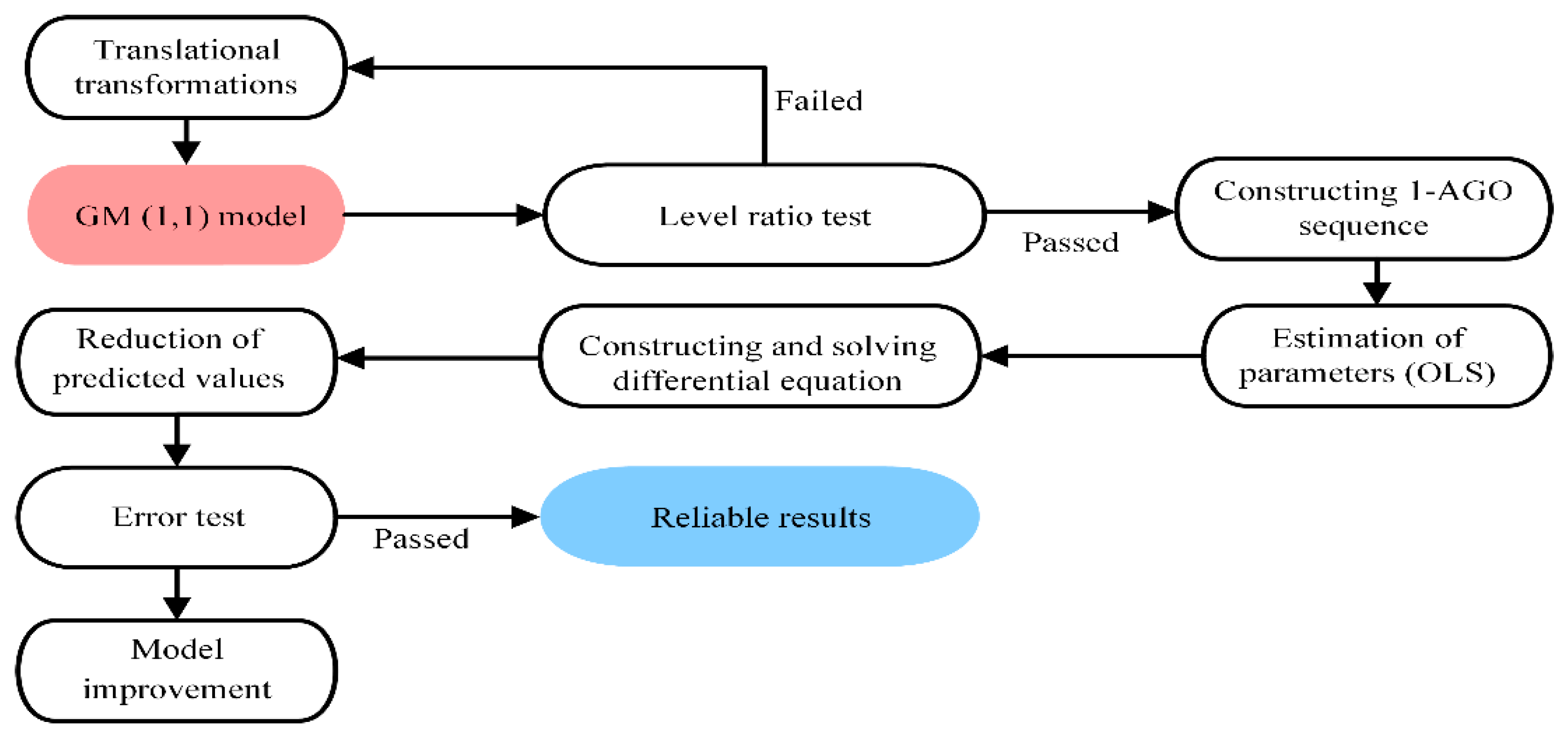
The basic principle of the GM (1, 1) prediction model can be summarized as follows. Firstly, we used the method of cumulative generation to make the data have specific laws. Then we established the first-order differential equation, solved it, and carried out the cumulative reduction in the result; the obtained value was the prediction value. The modelling procedure for the GM (1, 1) model is reflected in the framework diagram in Figure 2.
In this paper, the effectiveness of the model was evaluated using the mean absolute percentage error (MAPE) with the following formula:
M A P E = 1 n i = 1 n | x i 0 x i 1 | x i 0 × 100 %
If MAPE < 20%, the level of accuracy in the model projections could be considered as general requirements; if MAPE < 10%, the precision of the model forecasts could be considered to be high [45].

3. Results

3.1. Calculation Results

3.1.1. Calculation of ecc in Gansu Province in 2020

Through the above analysis of the emergy theory, the region’s total emergy is the accumulation of the maximum of four types of emergy. According to [36] and the emergy conversion coefficient, we could calculate the ecc in Gansu Province in 2020 as shown in Table 2.
From Table 2, we can obtain that the maximum value of solar emergy corresponding to the first four types of emergy was rain potential energy and that the sum of the ecc of rain potential energy and the energy of Earth’s rotation was 7.54 hm2, and considering 12% of the land was for biodiversity conservation, the ecc was 6.64 hm2 in 2020. The total emergy of Gansu Province was 5.85 × 10²² sej, the emergy density of the area was the proportion of its total emergy relative to its total area, and the emergy density in 2020 was
p = 5.85 × 10 22 4.26 × 10 7 1.37 × 10 15 sej / hm 2 .

3.1.2. Calculation of eef in Gansu Province for 2020

Among the six land types, the agricultural land mainly produced wheat, grain, beans, corn, potatoes, cotton, sugar beets, vegetables, and oilseed, and the highest yield of the agricultural land was vegetables at 1.48 × 10⁷ t in 2020. The woodland mainly produced fruits at 4.81 × 10⁶ t. The data of the grassland mainly came from meat; poultry; and eggs, milk, and wool of which the highest yield was meat at 1.10 × 10⁶ t. The water area produced aquatic products. The fuel land mainly produced coke, gasoline, and diesel (all three energy sources are not very different). The building land was mainly used for electricity. In 2020, the number of people in Gansu Province was 25,012,200, and the average annual precipitation was 506.5 mm [41]. The calculation of the eef could be obtained in Gansu Province as shown in Table 3. (The unit of the conversion factor for each item is J/t except for electricity, and the unit of the conversion factor for electricity is J/KW. Similarly, the unit of the original data is t except for electricity, and the unit of electricity is KWH.)
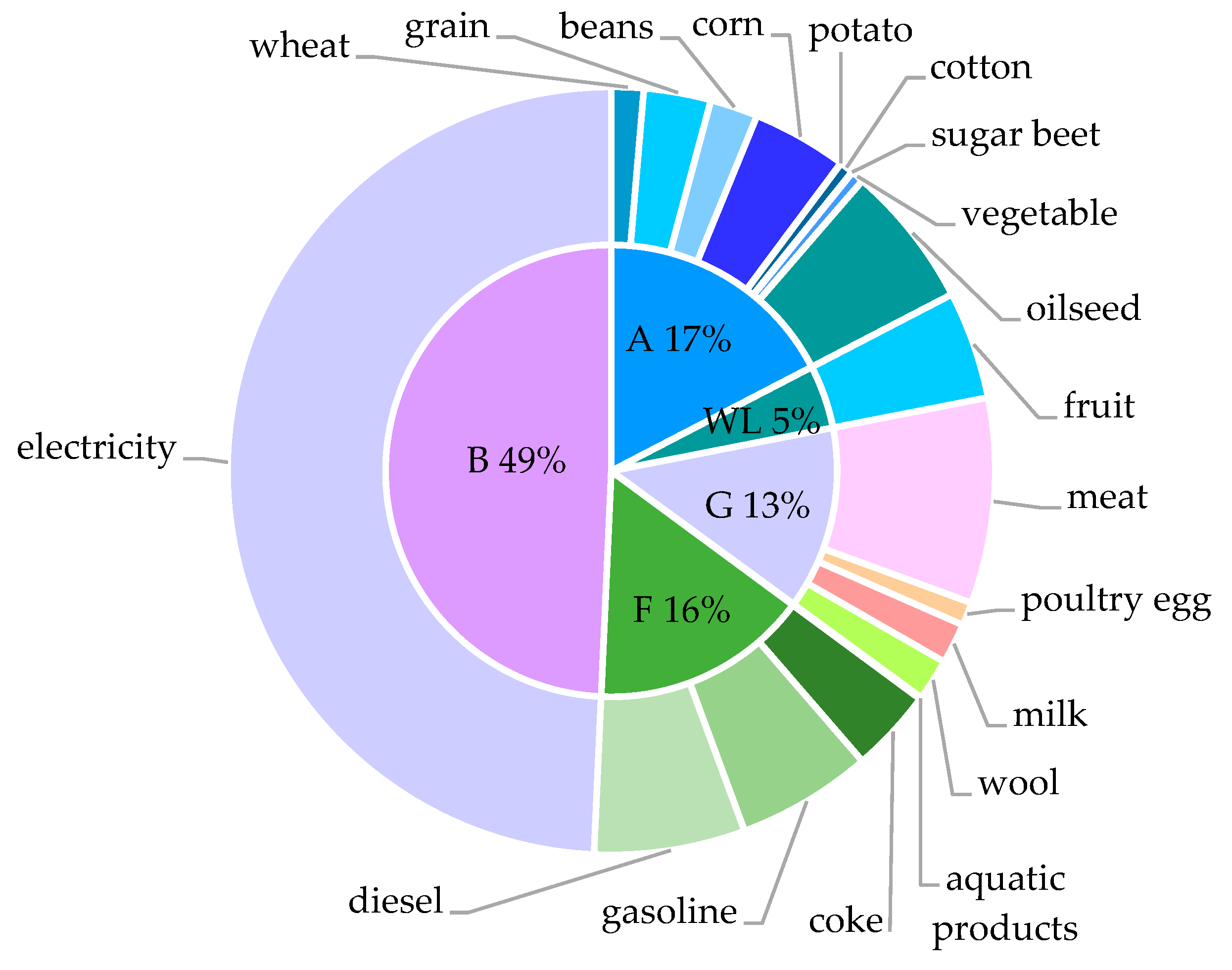
From Table 3, we can derive the relationship between the eef values among all the land types: building land (2.67 hm2) > agricultural land (9.24 × 10⁻¹ hm2) > fuel land (8.45 × 10⁻¹ hm2) > grassland (7.10 × 10⁻¹ hm2) > woodland (2.46 × 10⁻¹ hm2) > water area (3.78 × 10⁻³ hm2). The eef of Gansu Province in 2020 was 5.40 hm2.
We can see from Table 3 and Figure 3 that the use of the six land types in 2020 was highest for the building land, which was related to the fast economic development of Gansu Province since 2000. Then, the use for the agricultural land, fuel land, grassland, and woodland were relatively close. Gansu Province is rich in coal resources and fossil resources, which are widely used for industrial production, but the over-use of coal resources can cause serious pollution to other natural resources in the region and can affect sustainability. The use of the grassland and woodland was also high to accommodate the development of livestock farming. As Gansu Province is in the interior of China, the province is mountainous and wooded, so its use of water was the lowest of the six types.

3.1.3. Calculation of EEF3D in Gansu Province from 2001 to 2020

From Table 2 and Table 3, according to Equations (3)–(9), we can obtain that the EEF in 2020 was 1.35 × 10⁸ hm2, the ECC was 1.66 × 10⁸ hm2, the EEFsize was 1.35 × 10⁸ hm2, and the EEFdepth was 1; therefore, the EEF3D was 1.35 × 10⁸ hm2. Furthermore, five indicators were calculated for the remaining years following the same methodology and are given in Table 4 [46]:
Table 4 shows the trends in the ECC, EEF, EEFsize, EEFdepth, and EEF3D in Gansu Province from 2001 to 2020. It was found that the ECC varied between 1.20 × 10⁸ hm2 and 1.70 × 10⁸ hm2 throughout the process, with the ECC in 2002 being the minimum value throughout the process and reaching the maximum value in 2018. The EEF, EEFsize, and EEF3D show an over-all upward trend, with the EEF3D increasing from a minimum of 5.98 × 10⁷ hm2 in 2001 to a maximum of 1.41 × 10⁸ hm2 in 2015, an increase of 136%. Table 4 also reflects the ecological resource situation. Since 2001, ecological resources were almost in surplus, and only in 2015 and 2016 was there an ecological deficit. It is evident from Table 4 that the EEFdepth in 2015 and 2016 changed; the EEF over these two years was greater than the ECC, and the EEFdepth was more than one. This indicates that the natural resources were over-utilized during this period, requiring the depletion of the natural capital stock and an ecological deficit. However, the values show that the EEFdepth over this time interval was not very different from one, implying that, although the natural capital flows did not satisfy the development needs of Gansu Province, the extent to which the natural capital stock was taken up was not significant. The increase in the EEFsize, on the other hand, indicates that Gansu Province was utilizing natural capital flows at an increasing extent from 2001 to 2020. Therefore, we concluded that the ecological resources were almost in a sustainable state from 2001 to 2020, but there was a need to continue to enhance the conservation of the environment and the rational use of natural resources.

3.2. Predicted Results

We used Eviews 10.0 to perform unit root tests and auto-correlation and partial auto-correlation analyses, and we then employed SPSS Statistics 21.0 to make predictions on the sequence of numbers and outputted the results.
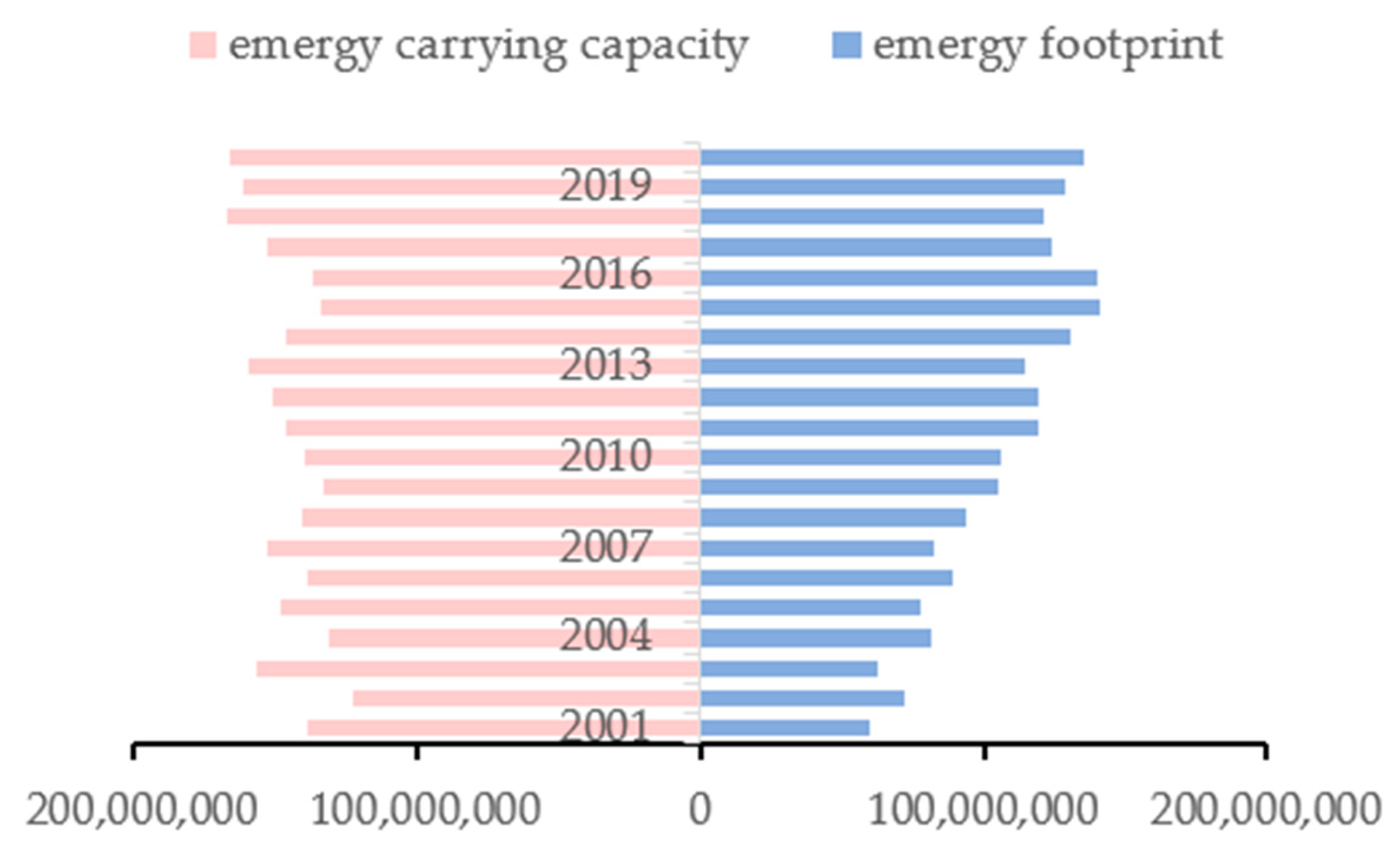
As can be seen from Figure 4, the ECC was constantly fluctuating between 1.00 × 10⁸ hm2 and 1.60 × 10⁸ hm2. It is not possible to visualize whether this is a smooth time series, and further software processing is required. The EEF series clearly increased year by year, which is not a smooth time series, and it requires transformation into a smooth time series.

3.2.1. Predicted Results of the ECC

In this section, data processing and the prediction of the ECC were carried out with the help of Eviews 10.0 and SPSS Statistics 21.0, and the predicted results were briefly analyzed.
By observing the trend in the ECC and the unit root test of the ECC, the original sequence of the ECC is non-stationary. The results were obtained by taking the natural logarithm of the sequence and the first-order difference as shown in Table 5:
From Table 5, we can obtain the p-values and t-values of the ECC, where p-values = 0.035 < 0.05 and where t-values were between 1% and 5%, indicating that the hypothesis was rejected at the 1% confidence interval. As the original sequence was stable after taking logarithms and first-order differences, the parameter d of the ARIMA model was one.
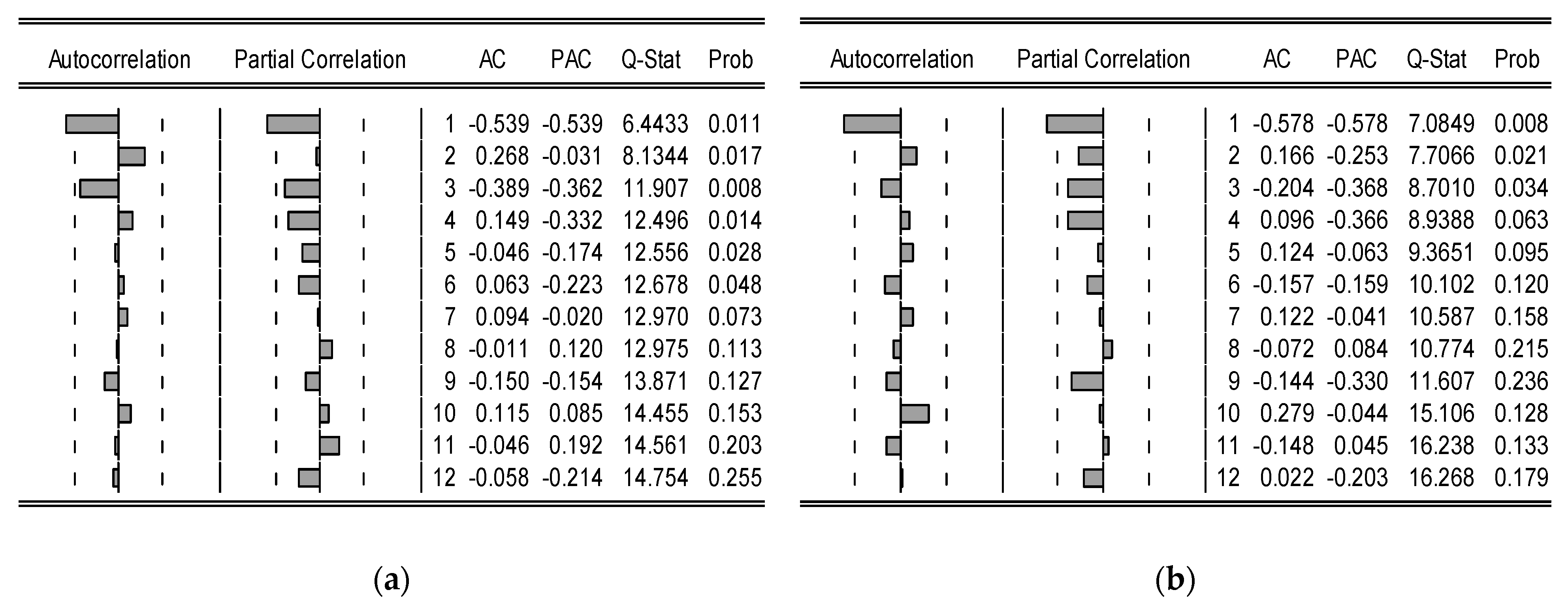
Through a graphical analysis of the auto-correlation coefficient and the partial auto-correlation coefficient, the values of the model parameters p and q could be determined so that a deterministic ARIMA (p, 1, q) model could be built for forecasting. As seen in Figure 5a, we finally chose the parameter combination with the smallest error, p = 1 and q = 4, after continuous simulation. On the other hand, the goodness of the model fit could be evaluated with the smooth R-squared and BIC values. A larger R-squared value and a lower BIC indicated a superior model fit. For model ARIMA (1,1,4), the smooth R-squared value was larger at 0.544, and the normalized BIC was 33.655. Therefore, the model fit was relatively good. In addition, we also predicted the ECC using the GM (1, 1) model, and the results were similar to those predicted by the ARIMA (1,1,4) model.
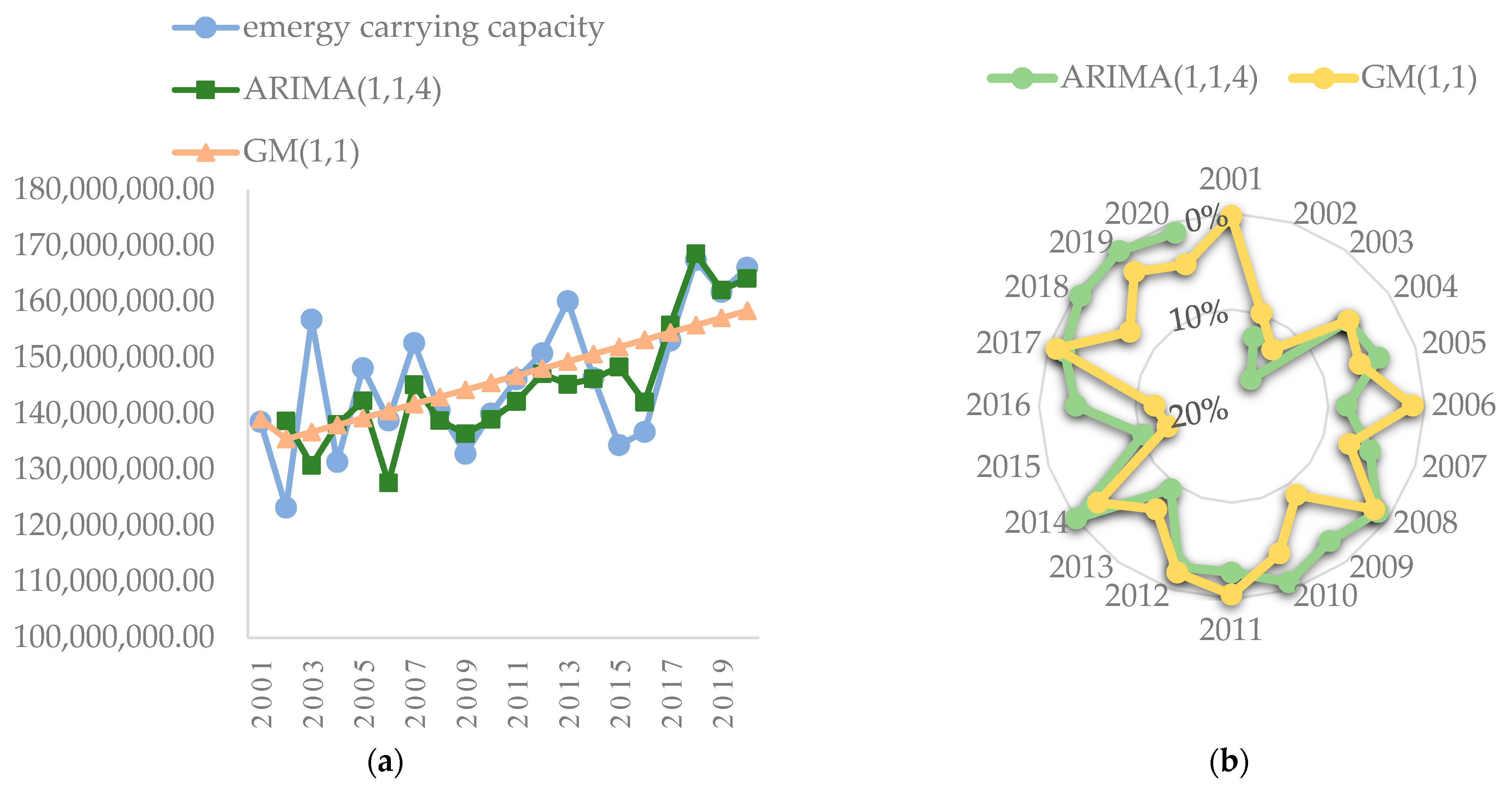
By viewing the graph comparing the actual and predicted values of the ECC in Gansu Province from 2001 to 2020 (Figure 6a), we can obtain that the predicted values of both models fluctuated up and down around the true levels. The predictions of the GM (1, 1) increased year by year, while the forecast values of the ARIMA (1,1,4) were more in line with changes in the actual values; both were in the range of 1.2 × 10⁸ hm2 and 1.65 × 10⁸ hm2 and varied constantly.
As can be seen from the error plots for both models (Figure 6b), the ARIMA (1,1,4) model had a maximum absolute percentage error of 16.6% (in 2003) and a minimum absolute percentage error of 0.1% (in 2014) for the predicted values, with all errors within 5%, except for in 2002, 2003, 2006, 2013, and 2015 when the errors exceeded 5%, and with a MAPE of 4.65%. The maximum absolute percentage error obtained from the GM (1, 1) model was 13.03% (in 2015), and the minimum absolute percentage error was 0.34% (in 2001), except for 2003, 2015, and 2016 when the absolute percentage error exceeded 10%; all errors were within 10%, with a MAPE of 5.45%. The MAPE of both models was less than 10%, which was a good fit that could accurately predict the changing trend in the ECC in the short term. In comparison, the ARIMA (1,1,4) predicted better results and could be used to forecast the ECC of Gansu Province from 2021 to 2030.
Finally, SPSS Statistics 21.0 was used to anticipate the ECC from 2021 to 2030 and to compare the predictions made by the GM (1, 1). In Figure 7a, the ARIMA (1,1,4) results increased year by year, while the ECC foreseen by the GM (1, 1) was stable around 1.60 × 10⁸ hm2. The trend toward increasing values over time was not significant, and the predictions of the ARIMA (1,1,4) were all greater than those of the GM (1, 1).

3.2.2. Predicted Results of the EEF

The same method was used to forecast the EEF of Gansu Province over the period of 2021–2030. Firstly, the original series can be seen to have increased gradually with the increase in years and was a non-stationary series, and the unit root test was conducted after the second-order difference of the original series, which is shown in the Table 5.
The p-value = 0.08 < 0.1, and t-values between 5% and 10% are obtained from Table 5, indicating that the hypothesis was rejected at a confidence interval of 1%. The series after the second-order difference was essentially smooth, so the parameter d could be determined to take a value of two.
As shown in Figure 5b, the partial auto-correlation coefficients and auto-correlation coefficients gradually converged to near zero after one order at which point p and q both took the value of one. The error and normalized BIC of the ARIMA (1,2,1) could be obtained through multiple simulations and could be relatively minimal. We found a smoothed R-squared value of 0.525 and a BIC value of 33.24 at this point. In summary, it can be concluded that the ARIMA (1,2,1) model has a high accuracy and can be used for forecasting.
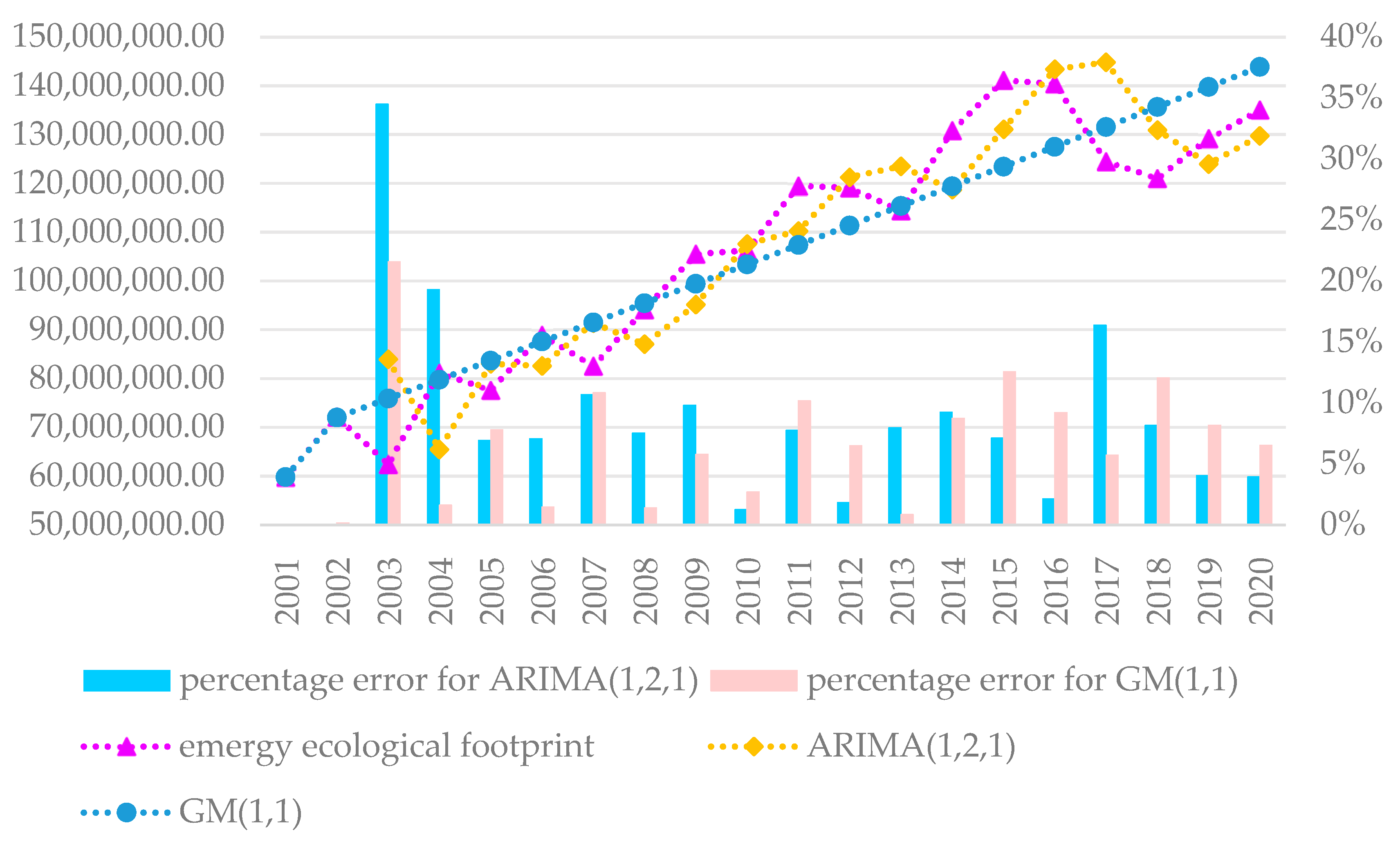
By observing the comparison of the true and forecast values of the EEF in Gansu Province from 2001 to 2020 (Figure 8), we can see that the changes in the predicted values of both models were basically in line with the trends in the actual values. The six-point predictions of the GM (1, 1) almost over-lapped with the original data, whereas the predictions of the ARIMA (1,2,1) only over-lapped with the original data at three points.
As can be seen from Figure 8, the maximum absolute percentage error of the predicted values from the ARIMA (1,2,1) model was 34.49% (in 2003), and the minimum absolute percentage error was 1.25% (in 2010), with most of the errors within 10% and a MAPE of 9.2%. The maximum absolute percentage error of the predicted values obtained from the GM (1, 1) model was 21.57% (in 2003), and the minimum absolute percentage error was 0.01% (in 2001), with most of the errors distributed within 5% and a MAPE of 6.69%. The MAPE values of both models were less than 10%, and the forecasting accuracy was high. According to the results, the GM (1, 1) model predicts relatively good results and could be utilized to predict the EEF from 2021 to 2030.
From Figure 7b, the EEF values predicted by the GM (1, 1) model were, over-all, larger than those predicted by the ARIMA (1,2,1) model, and the two models predicted the same trend, i.e., the EEF increasing year by year from 2021 to 2030.

3.2.3. Predicted Results of the EEF3D

As the EEF3D is calculated by the ECC and EEF, selecting a suitable prediction model improves the accuracy of the EEF3D projections. Therefore, the predicted ECC series using the ARIMA (1,1,4) and the predicted EEF series using the GM (1, 1) were chosen to anticipate the EEF3D of Gansu Province from 2021 to 2030, and the projections are shown in Table 6.
The corresponding EEFsize, EEFdepth, and EEF3D were calculated from the predicted ECC and EEF of Gansu Province from 2021 to 2030. From Table 6, it can be obtained that the EEFdepth was always one, and the EEFsize and EEF always remained the same. Therefore, based on the equations of the EEFsize and EEFdepth, we know that the EEF3D is equal to the EEF and the ECC is always greater than the EEF. From the changing trend, the ECC, EEF, and EEF3D showed a steadily increasing trend year by year. In summary, Gansu Province will be in an ecological surplus from 2021 to 2030, and the natural capital flow can meet the development needs of Gansu Province. Even so, we must insist on the peaceful cohabitation of human beings and nature; respect nature, follow nature, and protect wildlife.

4. Discussion

4.1. Analysis of Results and Comparison

According to the above calculation and analysis of the ECC, EEF, EEFdepth, EEFsize, and EEF3D in Gansu Province from 2001 to 2020, the EEF is developing much quicker than the ECC. Indeed, both the ECC and EEF are steadily increasing, and relevant authorities are actively taking scientific and rational management measures, such as using technology to improve the utilization of natural energy sources such as wind and tidal energy and effectively increasing agricultural production, which will result in an increase in the ECC. However, according to the above calculations and projections, the ECC in 2030 will be approximately 1.53 times that of 2001, the EEF in 2030 will be approximately 3.11 times that of 2001, and the EEF3D in 2030 will be approximately 3.11 times that of 2001, indicating that human socioeconomic activities are rapidly developing and that the continuous growth of the footprint is putting enormous pressure on natural capital. This finding is supported by [28] and by studies released by the Global Footprint Network [47]. Furthermore, the ECC in 2015 and 2016 was less than the EEF, and natural ecosystems were temporarily in deficit, necessitating the adjustment of the EEF in time, a conclusion similar to the findings of [26].
We discovered that the percentage of the building land among the six land types is an important indicator of the influence on the footprint, and, in 2020, for example, the share of the building land in the eef reached 49%, much greater than the other five land types. This also represented Gansu Province’s rapid economic development over the previous 20 years, the quickening process of industrialization and modernization, and the necessity to adapt the industrial structure in a timely way at the appropriate time as shown by research [39].

4.2. Limitations and Applications of the Model

Through research and comparison, the model shows certain shortcomings. Natural capital supply and demand on various types of biologically productive land have not been studied. The values derived for EEFdepth following the computation in this work may be slightly lower than the real values since the accumulation of the EEF of the six land types leads to deficits in some land types being offset by surpluses in others. Although the ARIMA model and the GM (1, 1) model are widely applied to various industry sectors, this paper only used 20 years of data from Gansu Province as the basis for prediction, and the sample size needs to be more significant. Therefore, there is an inevitable error between the predicted and actual values. However, the prediction accuracy is relatively high and more aligned with the actual situation. Therefore, the 3D EEF model proposed in this paper can be a reference for the construction of the ecological economy in Gansu Province.
Despite the model’s limitations, the examination of the calculations and predictions demonstrates that the model may give a scientific reference for analyzing the sustainability of ecological and economic systems and for altering the structure of ecological systems. Furthermore, the ecological footprint model has been applied to a variety of domains, including population increases [28], commodity prices [48], GDP [49,50], and so on. In future work, we will consider more models to make more accurate predictions of sustainability indicators in order to obtain more objective and comprehensive analysis results, which will provide effective measures for the sustainability of ecosystems.

4.3. Policy Implications

Based on the results of the above findings, the following strategies and recommendations for the ecologically sustainable development of Gansu Province are put forward. First, “The Belt and Road Initiative” construction should be promoted, and full play should be given to Gansu’s geographical, resource, and energy advantages. External exchanges and cooperation should be expanded, and greater efforts should be made to develop tourism, agriculture, and agricultural product processing to reduce the excessive and inefficient use of ecological resources. Second, the ecosystem structure must be adjusted so that each productive land type has an appropriate share of the total EEF. The area of land used for buildings must be reduced, and the rational and efficient use of the agricultural land, grassland, forest land, and fossil energy must be increased. Third, influenced by its topography and climate, Gansu Province is rich in clean energy resources (such as wind and solar energy), and it is important to make full use of the advantages of new energy, to improve the infrastructure for new energy development, and to optimize the construction of energy consumption. With the rapid increase in economic development in Gansu Province, investment in new energy should be increased year by year, reducing the consumption of fossil energy sources such as coal while increasing the use of new energy sources to achieve green, low-carbon, and high-quality development. Fourth, the livestock carrying capacity of the pastureland in Gansu Province should be reasonably estimated to prevent overgrazing. Advanced science and technology should be adopted to increase the ECC of the pastureland, grassland, and woodland and to promote the sustainable development of livestock farming. In addition, there is a need to strengthen the construction of fallow land, forestry, and grass; to control the population size; and to improve the public awareness of environmental protection and knowledge of energy conservation, among other effective strategies.

5. Conclusions

Since the theory of emergy analysis was proposed, it has been used to study a variety of fields, such as ecology, economy, and astronomy. Emergy analysis is of great practical and theoretical importance to quantify the resources and services of ecosystems, and it can be used to measure the human use of resources in ecosystems [51]. This paper combines the footprint size and depth in the 3D emergy ecological footprint model with the theory of emergy analysis and analyzes the ECC and EEF series of Gansu Province from 2001 to 2020 using the Eviews 10.0 software. The projections of the ECC, EEF, EEF3D, and ecosystem sustainability in Gansu Province from 2021 to 2030 were carried out using SPSS 21.0 software.
This study indicates that, in Gansu Province, the EEF3D had an over-all increase trend from 2001 to 2020 (except for in 2015 and 2016), the EEF was lower than ECC, and the EEFdepth = 1. This shows that the supply of natural resources could fulfill the needs of human social activities from 2001 to 2020, or that the natural ecological and economic system was in a surplus. In 2015 and 2016, the EEF was greater than the ECC, and the EEFdepth was greater than one, indicating that the demand for human socioeconomic development outpaced the flow of natural resources. The degree of human capital stock depletion increased with the EEF depth, which could result in ecological deficits and an unsustainable level of development. From the results of the ARIMA and GM (1, 1) models, the EEF3D of Gansu Province will steadily increase from 2021 to 2030, with an EEFdepth equal to one. According to the EEF3D formula, the amount of human appropriation of natural capital flows is growing, but the natural capital stock is not diminishing. Hence, the ecological economy will be in surplus. Nevertheless, a need to improve the effective utilization of environmental resources, to develop and utilize clean energy sources such as wind and solar energy, and to set the livestock industry that rationally still exists to promote sustainable ecological development.
The previously mentioned results have been analyzed, and recommendations for sustainable ecosystem development in Gansu Province have been produced. Because there is a big disparity in the EEF share of each land type in the region and because the EEF share of the agricultural land is gradually rising, the ecosystem structure must be adjusted over time to ensure an appropriate proportion of each land type. Furthermore, we need to improve the use of renewable energy, to optimize energy construction, and to limit our reliance on fossil fuels. In order to live in harmony with the environment, we must adopt a scientific consumption model and aggressively encourage green, low-carbon, and high-quality development.

Author Contributions

Conceptualization, H.L.; methodology, H.L.; software, X.L.; formal analysis, H.L.; data curation, J.W. and L.H.; writing—original draft, X.L. and J.W.; visualization, X.L.; funding acquisition, H.L. All authors have read and agreed to the published version of the manuscript.

Funding

This work was supported by the Research Fund for Humanities and Social Sciences of the Ministry of Education (20XJAZH006), the Gansu Science and Technology Fund (20JR5RA512), the Fundamental Research Funds for the Central Universities (31920230030), the Gansu Provincial Education Department’s Outstanding Graduate Student “Innovation Star” Project (2023CXZX-197) and the Leading Talents Project of the State Ethnic Affairs Commission of China.

Institutional Review Board Statement

Not applicable.

Informed Consent Statement

Not applicable.

Data Availability Statement

Data supporting reported results can be found in referenced publications.

Acknowledgments

We would like to thank Lei Yang of China University of Petroleum (Beijing) for his help in drawing up the Digital Elevation Model (DEM) map of the study area.

Conflicts of Interest

The authors declare no conflict of interest.

References

  1. Li, H.J.; Qu, J.S.; Pang, J.X.; Xu, L.; Han, J.Y. Spatial-temporal synthetic measurement of coupling coordination and sustainable development of population-economy-society-resource-environment system in Gansu Province. J. Arid Land 2020, 43, 1622–1634. [Google Scholar]
  2. Peng, W.J.; Wang, X.M.; Li, X.K.; He, C.C. Sustainability evaluation based on the emergy ecological footprint method: A case study of Qingdao, China, from 2004 to 2014. Ecol. Indic. 2018, 85, 1249–1261. [Google Scholar] [CrossRef]
  3. Liu, H.; Wei, Y.M.; Jin, X. Emergy footprint analysis of gannan Tibet an autonomous prefecture ecological-economic systems. In Ecosystem Assessment and Fuzzy Systems Management; Springer: Cham, Switzerland, 2014; pp. 53–61. [Google Scholar]
  4. Odum, H.T. Systems Ecology: An Introduction; John Wiley & Sons: New York, NY, USA, 1983. [Google Scholar]
  5. Wackernagel, M.; Rees, W. Our Ecological Footprint: Reducing Human Impact on the Earth; New Society Publishers: Gabriola Island, BC, Canada, 1998. [Google Scholar]
  6. Zhao, S.; Li, Z.Z.; Li, W.L. A modified method of ecological footprint calculation and its application. Ecol. Model. 2005, 185, 65–75. [Google Scholar] [CrossRef]
  7. Zhao, S.; Song, K.; Gui, F.; Cai, H.W.; Jin, W.H.; Wu, C.W. The emergy ecological footprint for small fish farm in China. Ecol. Indic. 2013, 29, 62–67. [Google Scholar] [CrossRef]
  8. Chen, B.; Chen, G.Q. Ecological footprint accounting based on emergy—A case study of the Chinese society. Ecol. Model. 2006, 198, 101–114. [Google Scholar] [CrossRef]
  9. Chen, C.F.; Wang, H.Y.; Xiao, D.N.; Wang, D.Q. Comparison of sustainable development status in Heilongjiang Province based on traditional ecological footprint method and emergy ecological footprint method. J. Appl. Ecol. 2008, 19, e2544–e2549. [Google Scholar]
  10. Mancini, M.S.; Galli, A.; Niccolucci, V.; Lin, D.; Bastianoni, S.; Wackernagel, M.; Marchettini, N. Ecological footprint: Refining the carbon footprint calculation. Ecol. Indic. 2016, 61, 390–403. [Google Scholar] [CrossRef]
  11. Lin, Q.P.; Feng, Z.S.; Liu, N.H.; Mei, Y. Modified Model of Ecological Footprint Accounting and Its Application to Cropland in Jiangsu, China. Pedosphere 2008, 18, 9. [Google Scholar]
  12. Liu, X.M.; Fu, J.Y.; Jiang, D.J.; Luo, J.W.; Sun, C.X.; Liu, H.M.; Wen, R.; Wang, X. Improvement of ecological footprint model in national nature reserve based on net primary production (NPP). Sustainability 2018, 11, 2. [Google Scholar] [CrossRef]
  13. Yang, Y.; Hu, D. Natural capital utilization based on a three-dimensional ecological footprint model: A case study in northern Shaanxi, China. Ecol. Indic. 2018, 87, 178–188. [Google Scholar] [CrossRef]
  14. Fang, K. Ecological footprint depth and size: New indicators for a 3D model. Acta Ecol. Sin. 2013, 33, 0267–0274. [Google Scholar] [CrossRef]
  15. Zhang, L.; Dzakpasu, M.; Chen, R.; Wang, X.C. Validity and utility of ecological footprint accounting: A state-of-the-art review. Sustain. Cities Soc. 2017, 32, 411–416. [Google Scholar] [CrossRef]
  16. Niccolucci, V.; Bastianoni, S.; Tiezzi, E.B.P.; Wackernagel, M.; Marchettini, N. How deep is the footprint? A 3D representation. Ecol. Model. 2009, 220, 2819–2823. [Google Scholar] [CrossRef]
  17. Niccolucci, V.; Galli, A.; Reed, A.; Neri, E.; Wackernagel, M.; Bastianoni, S. Towards a 3D national ecological footprint geography. Ecol. Model. 2011, 222, 2939–2944. [Google Scholar] [CrossRef]
  18. Fang, K.; Reinout, H. A review on three-dimensional ecological footprint model for natural capital accounting. Prog. Geogr. 2012, 31, 1700–1707. [Google Scholar]
  19. Fang, K.; Li, H.C. Provincial Pattern of China’s Natural Capital Use: A Modification and Application of Ecological Footprint Depth and Size. J. Nat. Resour. Policy Res. 2012, 27, 1995–2005. [Google Scholar]
  20. Fang, K. Changes in the spatial distribution of natural capital use among G20 countries from 1999 to 2008. Resour. Sci. 2014, 36, 793–800. [Google Scholar]
  21. Fang, K. Assessing the natural capital use of eleven nations: An application of a revised three-dimensional model of ecological footprint. Acta Ecol. Sin. 2015, 35, 3766–3777. [Google Scholar]
  22. Li, P.H.; Zhang, R.Q.; Xu, L.P. Three-dimensional ecological footprint based on ecosystem service value and their drivers: A case study of Urumqi. Ecol. Indic. 2021, 131, 108117. [Google Scholar] [CrossRef]
  23. Peng, J.; Du, Y.Y.; Ma, J.; Liu, Z.W.; Liu, Y.X.; Wei, H. Sustainability evaluation of natural capital utilization based on 3D EF model: A case study in Beijing City, China. Ecol. Indic. 2015, 58, 254–266. [Google Scholar] [CrossRef]
  24. Rudolph, A.; Figge, L. Determinants of Ecological Footprints: What is the role of globalization? Ecol. Indic. 2017, 81, 348–361. [Google Scholar] [CrossRef]
  25. Wackernagel, M.; Monfreda, C.; Erb, K.H.; Haberl, H.; Schulz, N.B. Ecological footprint time series of Austria, the Philippines, and South Korea for 1961-1999: Comparing the conventional approach to an ‘actual land area’ approach. Land Use Policy 2004, 21, 261–269. [Google Scholar] [CrossRef]
  26. Wu, F.F.; Yang, X.H.; Shen, Z.Y.; Bian, D.H.; Babuna, P. Exploring sustainability and decoupling effects of natural capital utilization in China: Evidence from a provincial three-dimensional ecological footprint. J. Clean. Prod. 2021, 295, 126486. [Google Scholar] [CrossRef]
  27. Wang, Z.H.; Lin, Y.G.; Yin, J.H.; Zhang, B. Assessment and prediction of environmental sustainability in China based on a modified ecological footprint model. Resour. Conserv. Recycl. 2017, 132, 301–313. [Google Scholar] [CrossRef]
  28. Lin, D.; Hanscom, L.; Murthy, A.; Galli, A.; Evans, M.; Neill, E.; Mancini, M.S.; Martindill, J.; Medouar, F.Z.; Huang, S.; et al. Ecological Footprint Accounting for Countries: Updates and Results of the National Footprint Accounts, 2012–2018. Resources 2018, 7, 58. [Google Scholar] [CrossRef]
  29. Long, X.Y.; Yu, H.J.; Sun, M.X.; Wang, X.C.; Kleme, J.J.; Xie, W.; Wang, C.; Li, W.; Wang, Y. Sustainability evaluation based on the Three-dimensional Ecological Footprint and Human Development Index: A case study on the four island regions in China. J. Environ. Manag. 2020, 265, 110509. [Google Scholar] [CrossRef] [PubMed]
  30. Hu, M.H.; Yuan, J.H.; Chen, L. Water ecological footprint size, depth and its spatial pattern correlation in the “Four-city Area in Middle China”. Ecol. Indic. 2021, 133, 108387. [Google Scholar] [CrossRef]
  31. Sun, C.Z.; Zhang, Z.X. Assessment of water ecological footprint size, depth, and spatial pattern in China. Acta Ecol. Sin. 2017, 37, 7048–7060. [Google Scholar]
  32. Poongodi, M.; Vijayakumar, V.; Chilamkurti, N. Bitcoin price prediction using ARIMA model. J. Internet Technol. 2020, 10, 396–406. [Google Scholar] [CrossRef]
  33. Wang, G.; Wang, J.L.; Su, B.L. Dynamic simulation and prediction of ecological footprint in Liaohe River Basin based on ARIMA model. J. Ecol. Environ. 2013, 22, 632–638. [Google Scholar]
  34. Zhang, B.; Liu, X.L. Dynamic ecological footprint simulation and prediction based on ARIMA Model: A case study of Gansu Province, China. Sheng Tai Xue Bao 2011, 31, 6251–6260. [Google Scholar]
  35. Ma, M.L.; Wang, Z.Z. Prediction of the energy consumption variation trend in South Africa based on ARIMA, NGM and NGM-ARIMA models. Energies 2019, 13, 10. [Google Scholar] [CrossRef]
  36. Li, J.X.; Chen, Y.N.; Xu, C.C.; Li, Z. Evaluation and analysis of ecological security in arid areas of Central Asia based on the emergy ecological footprint (EF) model. J. Clean. Prod. 2019, 235, 664–677. [Google Scholar] [CrossRef]
  37. Deng, J.L. Control problems of grey systems. Syst. Control Lett. 1982, 1, 288–294. [Google Scholar]
  38. Chen, H.S. Evaluation and analysis of eco-security in environmentally sensitive areas using an emergy ecological footprint. Int. J. Environ. Res. Public Health 2017, 14, 136. [Google Scholar] [CrossRef]
  39. Liu, H.; Li, D.Y.; Ma, R.; Ma, M. Assessing the ecological risks based on the three-dimensional ecological footprint model in Gansu Province. Sustainability 2022, 14, 16995. [Google Scholar] [CrossRef]
  40. National Energy Administration. Available online: http://www.nea.gov.cn/2021-07/23/c_1310080005.htm (accessed on 21 March 2023).
  41. The Editorial Board of Gansu Statistical Yearbook in Gansu Province. In Gansu Statistical Yearbook 2001–2020; Statistics Press: Beijing, China, 2021.
  42. Odum, H.T. Self-organization, transformity, and information. Science 1988, 242, 1132–1139. [Google Scholar] [CrossRef]
  43. Guizhou Energy Administration. Available online: http://nyj.guizhou.gov.cn/zxfw/nyzs/ (accessed on 22 March 2023).
  44. Odum, H.T. Environment Accounting: Energy and Environment Decision Making; John Wiley: New York, NY, USA, 1996. [Google Scholar]
  45. Wang, Z.X.; Li, D.D.; Zheng, H.H. Model comparison of GM (1, 1) and DGM (1, 1) based on Monte-Carlo simulation. Phys. A 2020, 542, 123341. [Google Scholar] [CrossRef]
  46. Lin, X.F.; Liu, H.; Wei, J.H. Research on Sustainable Development in Gansu Province Based on Three-Dimensional Energy Footprint. In Proceedings of the 3rd International Conference on Green Energy, Environment and Sustainable Development (GEESD2022), Online, 29 June 2022, 3rd ed.; IOS Press BV: Amsterdam, The Netherlands, 2022; pp. 422–428. [Google Scholar]
  47. Global Footprint Network. Obtenido de Global Footprint Network. Available online: http://www.footprintnetwork.org (accessed on 22 March 2023).
  48. Galli, A.; Halle, M.; Grunewald, N. Physical limits to resource access and utilisation and their economic implications in Mediterranean economies. Environ. Sci. Policy 2015, 51, 125–136. [Google Scholar] [CrossRef]
  49. Niccolucci, V.; Pulselli, F.M.; Tiezzi, E. Strengthening the threshold hypothesis: Economic and biophysical limits to growth. Ecol. Econ. 2007, 60, 667–672. [Google Scholar] [CrossRef]
  50. Bastianoni, S.; Niccolucci, V.; Neri, E.; Cranston, G.; Galli, A.; Wackernagel, M. Sustainable Development: Ecological Footprint in Accounting. In Encyclopedia of Environmental Management; CRC Press: Boca Raton, FL, USA, 2013; pp. 2467–2481. [Google Scholar]
  51. Hau, J.L.; Bakshi, B.R. Promise and problems of emergy analysis. Ecol Model. 2004, 178, 215–225. [Google Scholar] [CrossRef]
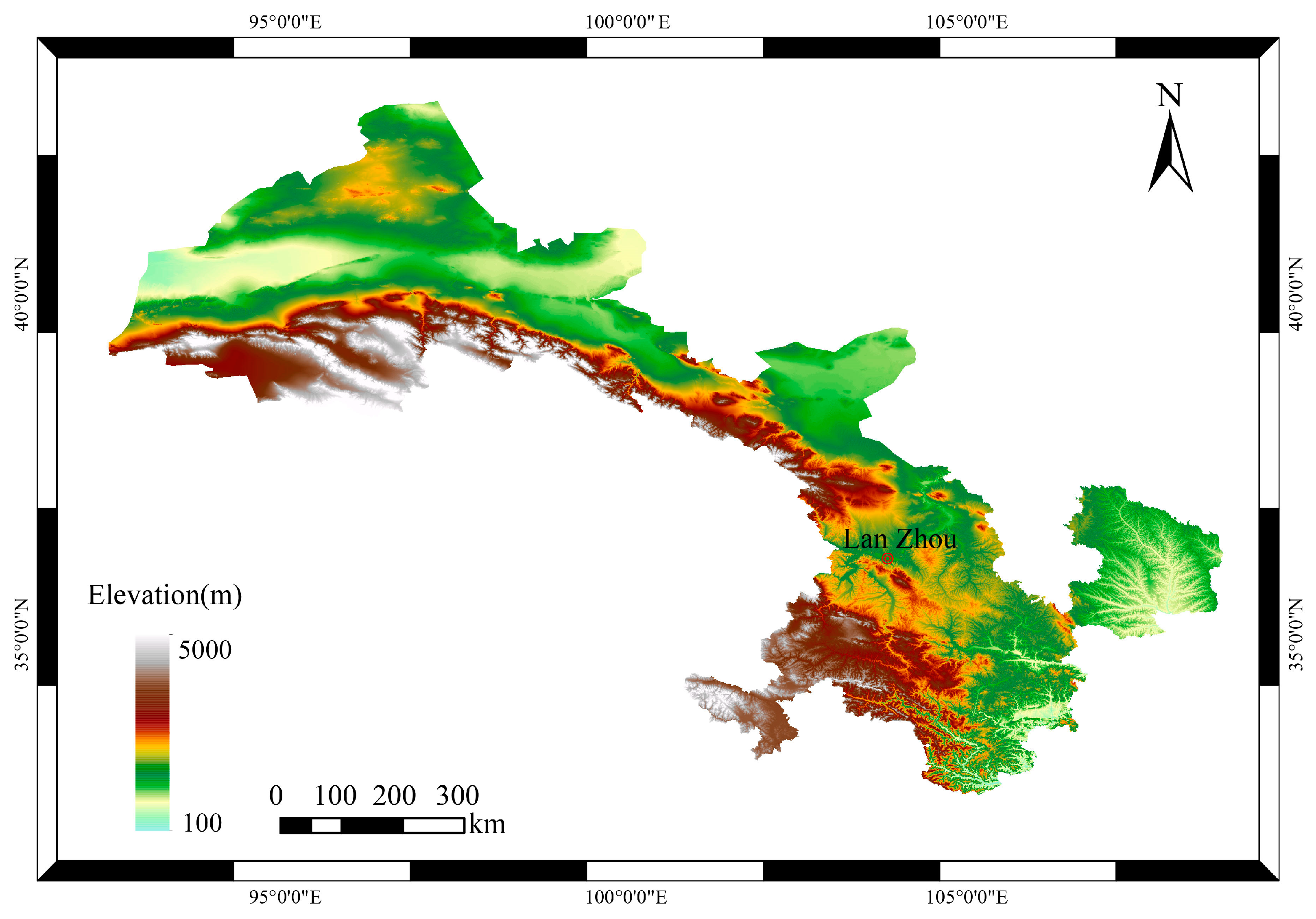
Figure 1. Study area.
Sustainability 15 08007 g001
Figure 2. GM (1, 1) model flowchart.
Sustainability 15 08007 g002
Figure 3. Percentage of the eef of each land type. (A is agricultural land, B is building land, F is fuel land, G is grassland, W is water area, and WL is woodland.
Sustainability 15 08007 g003
Figure 4. Trends in ECC and EEF in Gansu Province from 2001 to 2020.
Sustainability 15 08007 g004
Figure 5. Correlation coefficient diagram. (a) Correlation coefficient diagram of ECC and (b) correlation coefficient diagram of EEF.
Sustainability 15 08007 g005
Figure 6. Fitting results for the ECC from 2001 to 2020. (a) Comparison of the fitted results with the original data and (b) percentage error for both models at each time point.
Sustainability 15 08007 g006
Figure 7. The projections of Gansu Province for 2021–2030. (a) Projections of ECC and (b) projections of EEF.
Sustainability 15 08007 g007
Figure 8. Fitting results for the EEF from 2001 to 2020.
Sustainability 15 08007 g008
Table 1. Gansu Province EEF account type and data sources.
Account TypeLand TypeIndicatorsData Source
Biological accountAgricultural landWheat, grain, beans, corn, potatoes, cotton, sugar beets, vegetables, and oilseedGansu Statistical Yearbook (2001–2020) [41]
Building landElectricity
Fuel landCoke, gasoline, and diesel
GrasslandMeat, poultry eggs, milk, and wool
Water areaAquatic products
WoodlandFruits
Table 2. Calculate the ecc of Gansu Province in 2020.
ItemOriginal Data
J
Emergy Transformity
sej/J
Solar Emergy
sej
Per-Capita Emergy
sej/cap
ecc
hm2/cap
Solar radiant energy2.38 × 10211.002.38 × 10219.52 × 10130.31
Wind energy3.30 × 10186.32 × 1022.09 × 10218.35 × 10130.27
Rain potential energy4.56 × 10188.89 × 1034.06 × 10221.62 × 10155.23
Chemical energy of rainwater1.07 × 10181.82 × 1041.94 × 10227.75 × 10142.50
Energy of Earth’s rotation6.18 × 10172.90 × 1041.79 × 10227.16 × 10142.31
Total emergy of the region 5.85 × 10²²
Table 3. Calculate the eef of Gansu Province in 2020.
Productive Land TypeSubjectConversion FactorOriginal DataEmergy Transformity sej/JSolar Emergy /sejci/sejeef /hm2
A *wheat1.38 × 10102.69 × 1066.80 × 1042.52 × 10211.01 × 10147.36 × 10-2
grain1.55 × 10109.42 × 1063.59 × 1045.24 × 10212.10 × 10141.53 × 10−1
beans2.07 × 10103.72 × 1056.90 × 1055.31 × 10212.13 × 10141.09 × 10−1
corn1.46 × 10106.17 × 1065.81 × 1045.23 × 10212.09 × 10142.17 × 10−1
potatoes4.20 × 1092.23 × 1062.70 × 1032.53 × 10191.01 × 10127.37 × 10−4
cotton1.88 × 10103.01 × 1041.90 × 1061.08 × 10214.30 × 10133.14E × 10−2
sugar beets2.50 × 1092.24 × 1058.49 × 1044.76 × 10191.90 × 10121.39E × 10−3
vegetables2.51 × 1091.48 × 1072.70 × 1041.00 × 10214.01 × 10132.92 × 10−2
oilseed2.64 × 10106.15 × 1056.90 × 1051.12 × 10224.48 × 10143.27 × 10−1
WL *fruits3.30 × 1094.81 × 1065.30 × 1058.41 × 10213.36 × 10142.46 × 10−1
G *meat4.60 × 1091.10 × 1063.17 × 1061.61 × 10226.42 × 10144.69 × 10−1
poultry eggs4.60 × 1091.98 × 1052.00 × 1061.82 × 10217.28 × 10135.32 × 10−2
milk3.20 × 1095.84 × 1051.70 × 1063.18 × 10211.27 × 10149.28 × 10−2
wool2.09 × 10103.56 × 1044.40 × 1063.27 × 10211.31 × 10149.55 × 10−2
W *aquatic products4.61 × 1091.41 × 1042.00 × 1061.30 × 10205.18 × 10123.78 × 10−3
F *coke3.18 × 10105.17 × 1063.98 × 1046.54 × 10212.62 × 10141.91 × 10−1
gasoline4.66 × 10104.51 × 1065.04 × 1041.06 × 10224.23 × 10143.09 × 10−1
diesel3.30 × 10105.43 × 1066.60 × 1041.18 × 10224.72 × 10143.45 × 10−1
B *electricity3.60 × 1061.60 × 10111.59 × 1059.17 × 10223.66 × 10152.67
eef/hm2 5.40
* A note on Table 3: A is agricultural land, B is building land, F is fuel land, G is grassland, W is water area, and WL is woodland.
Table 4. Five indicators for 3D EEF model from 2001 to 2020.
TimeECC/hm2EEF/hm2EEFsize/hm2EEFdepthEEF3D/hm2Ecological Status
20011.39 × 1085.98 × 1075.98 × 10715.98 × 107surplus
20021.23 × 1087.21 × 1077.21 × 10717.21 × 107surplus
20031.57 × 1086.24 × 1076.24 × 10716.24 × 107surplus
20041.31 × 1088.11 × 1078.11 × 10718.11 × 107surplus
20051.48 × 1087.76 × 1077.76 × 10717.76 × 107surplus
20061.39 × 1088.89 × 1078.89 × 10718.89 × 107surplus
20071.53 × 1088.26 × 1078.26 × 10718.26 × 107surplus
20081.41 × 1089.41 × 1079.41 × 10719.41 × 107surplus
20091.33 × 1081.06 × 1081.06 × 10811.06 × 108surplus
20101.40 × 1081.06 × 1081.06 × 10811.06 × 108surplus
20111.46 × 1081.19 × 1081.19 × 10811.19 × 108surplus
20121.51 × 1081.19 × 1081.19 × 10811.19 × 108surplus
20131.60 × 1081.14 × 1081.14 × 10811.14 × 108surplus
20141.46 × 1081.31 × 1081.31 × 10811.31 × 108surplus
20151.34 × 1081.41 × 1081.34 × 1081.0501.41 × 108deficit
20161.37 × 1081.40 × 1081.37 × 1081.0271.40 × 108deficit
20171.53 × 1081.24 × 1081.24 × 10811.24 × 108surplus
20181.67 × 1081.21 × 1081.21 × 10811.21 × 108surplus
20191.62 × 1081.29 × 1081.29 × 10811.29 × 108surplus
20201.66 × 1081.35 × 1081.35 × 10811.35 × 108surplus
Table 5. Unit root test for ECC and EEF based on Eviews 10.0.
SequenceADF Statistic
(t-Statistic)
Critical ValuesProb
1%5%10%
ECC−4.067−4.886−3.829−3.3630.035
EEF−3.547−5.125−3.933−3.4200.085
Table 6. The EEF3D forecast for Gansu Province from 2021 to 2030.
YearEEFsize/hm2EEFdepth/hm2EEF3D/hm2Ecological Status
20211.48 × 1081.001.48 × 108surplus
20221.52 × 1081.001.52 × 108surplus
20231.56 × 1081.001.56 × 108surplus
20241.60 × 1081.001.60 × 108surplus
20251.65 × 1081.001.65 × 108surplus
20261.69 × 1081.001.69 × 108surplus
20271.73 × 1081.001.73 × 108surplus
20281.77 × 1081.001.77 × 108surplus
20291.82 × 1081.001.82 × 108surplus
20301.86 × 1081.001.86 × 108surplus
Disclaimer/Publisher’s Note: The statements, opinions and data contained in all publications are solely those of the individual author(s) and contributor(s) and not of MDPI and/or the editor(s). MDPI and/or the editor(s) disclaim responsibility for any injury to people or property resulting from any ideas, methods, instructions or products referred to in the content.