
Influence of Limit State Function’s Form of Geotechnical Structures on Approximate Analytical Reliability Methods


Abstract
1. Introduction
2. FOSM
3. FORM
4. PEM
4.1. Estimating Statistical Moments
4.2. Fourth Moment Methods
5. Illustrative Examples
5.1. Example I: Floating Pile Embedded in Two-Layer Soil
5.2. Example II: Gravity Retaining Wall
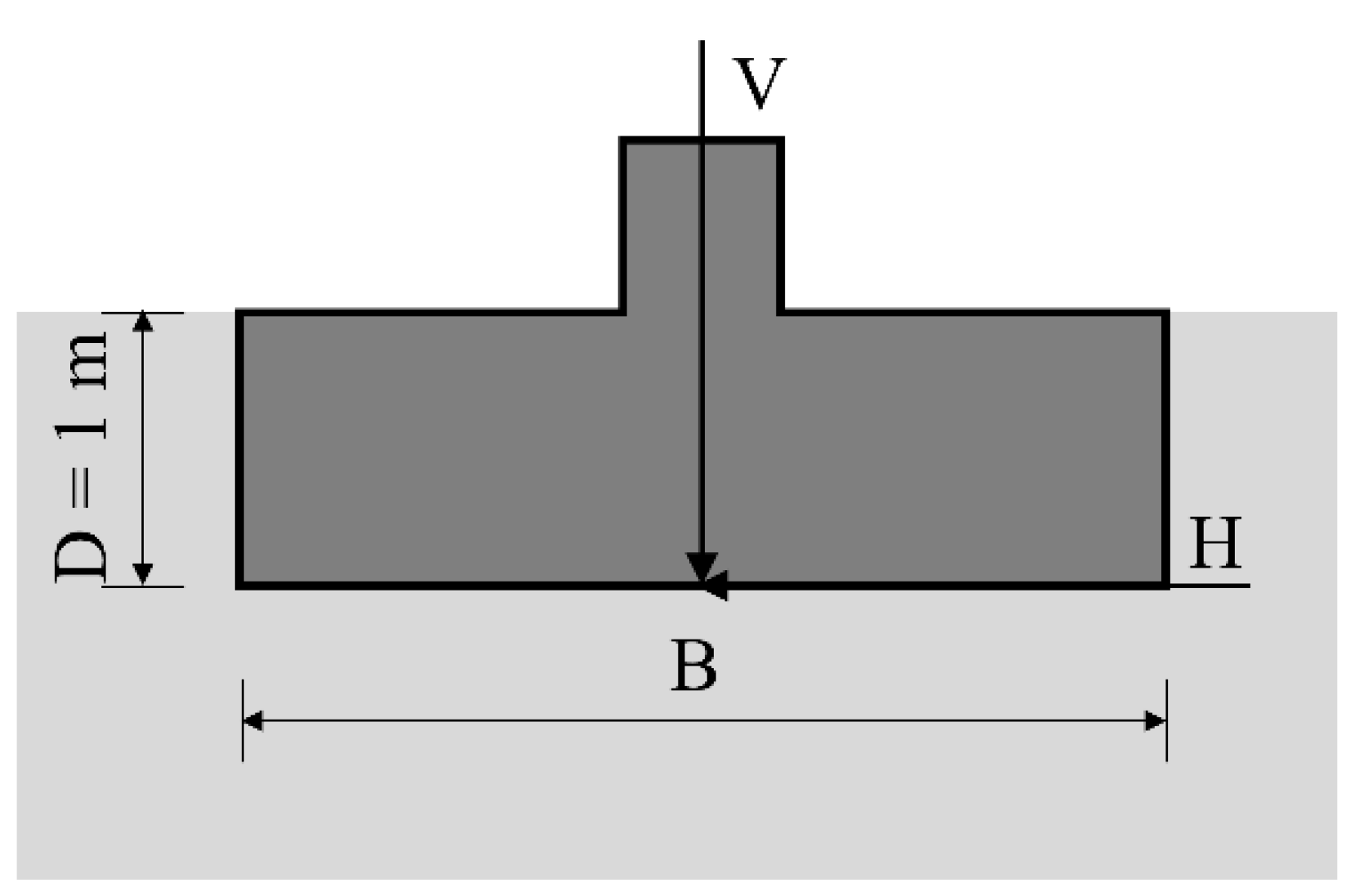
5.3. Example III: Square Footing
5.4. Example IV: Active Lateral Forces on Retaining Walls
5.5. Example V: A Homogeneous Clay Slope
6. Conclusions
- The form of LSF does not affect the accuracy of β obtained by FORM; however, it affects the computational efficiency of FORM. The accuracy of β obtained by FORM may be affected by the initial iteration point used in the optimization algorithms. When FORM is used for estimating the β of geotechnical structures, one should exercise caution on the initial iteration point to avoid obtaining unreasonable results. A practical suggestion is to try different initial iteration points to cross-validate the result of FORM.
- FOSM is sensitive to forms of LSF. Generally, FOSM can obtain more accurate estimation results with the logarithmic form of LSF compared with other forms. The computational efficiency of FOSM is independent of the form of LFS but dependent on the dimension of random variables. It is recommended to use the logarithmic form of LSF when FOSM is used to estimate the β of the geotechnical systems.
- The investigated PEMs are also sensitive to forms of LSF. Similar to FOSM, PEMs can also obtain more accurate estimation results with the logarithmic form of LSF compared with other forms. The computational efficiency of PEMs is dependent on the dimension of the random variable. PEMs may yield extremely large estimation errors due to the large number of random variables or complex correlations among random variables. Choosing a different but equivalent form of LSFs can sometimes avoid the inherent limitations of FM2 and FM3, where the Pearson system does not have a solution.
- All investigated examples show that the logarithmic form G = ln(R/L) is always the optimal choice among the four equivalent forms for the approximate reliability methods that are sensitive to the forms of LSFs. The probability distribution type, number of variables involved in the LSF, and level of coefficient of variation of the random variables have effects on the reliability indexes estimated by different forms of LSFs; however, they do not affect the result that the logarithmic form of the LSF is superior to the other forms. It should be noted that this result is not guaranteed theoretically but is supported by analyzing the five typical geotechnical examples. There may be some rare exceptions or specific limits that violate the result. For general cases, the logarithmic form G = ln(R/L) is recommended for the approximate reliability analysis methods.
Author Contributions
Funding
Institutional Review Board Statement
Informed Consent Statement
Data Availability Statement
Acknowledgments
Conflicts of Interest
Nomenclature
| List of symbols | |||
| β | reliability index | N | sand layer’s SPT-N value |
| Pf | probability of failure | εα | model transformation uncertainties |
| G | limit state function | εN | model transformation uncertainties |
| R | resistance | HT | retaining wall’s total height |
| L | load | t | thickness of concrete base and stem |
| X | random variables | γc | unit weight of concrete |
| X | vector of X | ϕb′ | effective friction angle of base sand |
| σX | standard deviation of X | ϕf | effective friction angle of the backfill sand |
| μX | mean of X | γf | unit weight of the backfill sand |
| CX | covariance matrix of X | Ka | coefficient of active earth pressure |
| H | gradient vector | D | embedment depth |
| U | independent standard normal random variables | γ | unit weight of soil |
| U | vector of U | V | vertical load |
| Gi | function of the i-th variable in X | H | horizontal load |
| Gμ | value of G(X) evaluated at μX | c | Cohesion |
| μi | mean of Gi | ϕ | Friction angle |
| σi | variance of Gi | ρ | Correlation coefficient |
| α3i | skewness of Gi | W | weight of footing concrete |
| α4i | kurtosis of Gi | N1,N2,N3 | Bearing capacity factors |
| μG | mean of G(X) | s1,s2,s3 | Shape factors |
| σG | variance of G(X) | d1,d2,d3 | Depth factors |
| α3G | skewness of G(X) | i1,i2,i3 | Inclination factors |
| α4G | kurtosis of G(X) | q | overburden or surcharge pressure at the footing |
| βSM | second-order moment reliability index | ||
| zu | standardized variables | COV | coefficient of variation |
| f(zu) | probability density function of zu | su(x,z) | the random field for su |
| Lc | thickness of clay layer | Δx | horizontal distances |
| Ls | thickness of sand layer | Δz | vertical distances |
| DL | dead loads | δx | horizontal scale of fluctuation |
| LL | live loads | δz | vertical scale of fluctuation |
| B | diameter of the pile/ Side length of square footing | F | lateral force |
| su LA | line average of su(x,z) along a potential slip line | ||
| Rc | resistances provided by clay layers | α | inclination angle of potential slip line |
| Rs | resistances provided by sand layers | Pa | active lateral force |
| su | undrained shear strength | Fs | factor of safety |
References
- Christian, J.T.; Ladd, C.C.; Baecher, G.B. Reliability applied to slope stability analysis. J. Geotech. Eng. 1994, 120, 2180–2207. [Google Scholar] [CrossRef]
- Jiang, S.-H.; Li, D.-Q.; Cao, Z.-J.; Zhou, C.-B.; Phoon, K.-K. Efficient system reliability analysis of slope stability in spatially variable soils using Monte Carlo simulation. J. Geotech. Geoenviron. Eng. 2015, 141, 4014096. [Google Scholar] [CrossRef]
- Jiang, S.-H.; Huang, J.; Griffiths, D.; Deng, Z.-P. Advances in reliability and risk analyses of slopes in spatially variable soils: A state-of-the-art review. Comput. Geotech. 2022, 141, 104498. [Google Scholar] [CrossRef]
- Zeng, P.; Jimenez, R.; Li, T. An efficient quasi-Newton approximation-based SORM to estimate the reliability of geotechnical problems. Comput. Geotech. 2016, 76, 33–42. [Google Scholar] [CrossRef]
- Zhang, W.; Goh, A.T.; Zhang, Y. Probabilistic assessment of serviceability limit state of diaphragm walls for braced excavation in clays. ASCE-ASME J. Risk Uncertain. Eng. Syst. Part A Civ. Eng. 2015, 1, 6015001. [Google Scholar] [CrossRef]
- Zheng, D.; Li, D.-Q.; Cao, Z.-J.; Tang, X.-S.; Phoon, K.-K. An analytical method for quantifying the correlation among slope failure modes in spatially variable soils. Bull. Eng. Geol. Environ. 2017, 76, 1343–1352. [Google Scholar] [CrossRef]
- Xiao, T.; Li, D.-Q.; Cao, Z.-J.; Tang, X.-S. Full probabilistic design of slopes in spatially variable soils using simplified reliability analysis method. Georisk Assess. Manag. Risk Eng. Syst. Geohazards 2017, 11, 146–159. [Google Scholar] [CrossRef]
- Yang, Z.; Ching, J. A novel simplified geotechnical reliability analysis method. Appl. Math. Model. 2019, 74, 337–349. [Google Scholar] [CrossRef]
- Wang, B.; Liu, L.; Li, Y.; Jiang, Q. Reliability analysis of slopes considering spatial variability of soil properties based on efficiently identified representative slip surfaces. J. Rock Mech. Geotech. Eng. 2020, 12, 642–655. [Google Scholar] [CrossRef]
- Zhang, J.; Huang, H.; Phoon, K. Application of the Kriging-based response surface method to the system reliability of soil slopes. J. Geotech. Geoenviron. Eng. 2013, 139, 651–655. [Google Scholar] [CrossRef]
- Li, D.-Q.; Xiao, T.; Cao, Z.-J.; Zhou, C.-B.; Zhang, L.-M. Enhancement of random finite element method in reliability analysis and risk assessment of soil slopes using Subset Simulation. Landslides 2016, 13, 293–303. [Google Scholar] [CrossRef]
- Liu, L.-L.; Deng, Z.-P.; Zhang, S.-H.; Cheng, Y.-M. Simplified framework for system reliability analysis of slopes in spatially variable soils. Eng. Geol. 2018, 239, 330–343. [Google Scholar] [CrossRef]
- Zevgolis, I.E.; Daffas, Z.A. System reliability assessment of soil nail walls. Comput. Geotech. 2018, 98, 232–242. [Google Scholar] [CrossRef]
- Yang, Z.; Liu, Y.; Nie, J.; Li, X. Efficient estimation of cumulative distribution functions of multiple failure modes using advanced generalized subset simulation. Int. J. Numer. Anal. Methods Geomech. 2022, 46, 1093–1108. [Google Scholar] [CrossRef]
- Zhang, J.; Zheng, Z.; Cai, Y.; Li, N.; Zhang, D. A FORM-based approach for probabilistic analysis in geotechnics: Application to a reinforced concrete drainage culvert. Int. J. Numer. Anal. Methods Geomech. 2019, 43, 2090–2105. [Google Scholar] [CrossRef]
- Chen, Z.; Du, J.; Yan, J.; Sun, P.; Li, K.; Li, Y. Point estimation method: Validation, efficiency improvement, and application to embankment slope stability reliability analysis. Eng. Geol. 2019, 263, 105232. [Google Scholar] [CrossRef]
- Fan, W.-L.; Wang, Y.-L.; Wei, Q.-K.; Yang, P.-C.; Li, Z.-L. Improved fourth-moment method for reliability analysis of geotechnical engineering. Rock Soil Mech. 2018, 39, 1463–1468. (In Chinese) [Google Scholar] [CrossRef]
- Yang, Z.; Ching, J. A novel reliability-based design method based on quantile-based first-order second-moment. Appl. Math. Model. 2020, 88, 461–473. [Google Scholar] [CrossRef]
- The Professional Standards Compilation Group of People’s Republic of China. SL 386-2007 Design Code for Engineered Slopes in Water Resources and Hydropower Projects; China Water Power Press: Beijing, China, 2007. [Google Scholar]
- Ministry of Construction of People’s Republic of China, Ministry of Water Resources and Bureau of Energy of People’s Republic of China. GB 50199-2013 Unified Standard for Reliability Design of Hydraulic Engineering Structures; China Planning Press: Beijing, China, 2013. [Google Scholar]
- ISO2394:2015; General Principles on Reliability of Structures. International Organization for Standardization: Geneva, Switzerland, 2015. Available online: https://www.iso.org/standard/58036.html (accessed on 10 May 2023).
- Zhao, Y.-G.; Ono, T. Moment methods for structural reliability. Struct. Saf. 2001, 23, 47–75. [Google Scholar] [CrossRef]
- Zhao, H. A practical and efficient reliability-based design optimization method for rock tunnel support. Tunn. Undergr. Space Technol. 2022, 127, 104587. [Google Scholar] [CrossRef]
- Pang, R.; Xu, B.; Zhou, Y.; Song, L. Seismic time-history response and system reliability analysis of slopes considering uncertainty of multi-parameters and earthquake excitations. Comput. Geotech. 2021, 136, 104245. [Google Scholar] [CrossRef]
- Phoon, K.-K. The story of statistics in geotechnical engineering. Georisk Assess. Manag. Risk Eng. Syst. Geohazards 2021, 14, 3–25. [Google Scholar] [CrossRef]
- Zhang, Z.; Li, Z.; Xu, G.; Gao, X.; Liu, Q.; Li, Z.; Liu, J. Lateral abutment pressure distribution and evolution in wide pillars under the first mining effect. Int. J. Min. Sci. Technol. 2023, 33, 309–322. [Google Scholar] [CrossRef]
- Low, B.; Einstein, H. Reliability analysis of roof wedges and rockbolt forces in tunnels. Tunn. Undergr. Space Technol. 2013, 38, 1–10. [Google Scholar] [CrossRef]
- Yang, Z.-Y.; Cao, Z.-J.; Feng, X.-B.; Li, D.-Q.; Au, S.-K. Robustness of subset simulation to functional forms of limit state functions in system reliability analysis: Revisiting and improvement. IEEE Trans. Reliab. 2017, 67, 66–78. [Google Scholar] [CrossRef]
- Bond, A.; Harris, A. Decoding Eurocode 7; Taylor & Francis: London, UK; New York, NY, USA, 2001. [Google Scholar] [CrossRef]
- Suchomel, R.; Mašı, D. Comparison of different probabilistic methods for predicting stability of a slope in spatially variable c–φ soil. Comput. Geotech. 2010, 37, 132–140. [Google Scholar] [CrossRef]
- Wu, Z.-Y.; Shi, Q.; Guo, Q.; Chen, J.-K. CST-based first order second moment method for probabilistic slope stability analysis. Comput. Geotech. 2017, 85, 51–58. [Google Scholar] [CrossRef]
- Duncan, J.M. Factors of safety and reliability in geotechnical engineering. J. Geotech. Eng. 2000, 126, 307–316. [Google Scholar] [CrossRef]
- Löfman, M.S.; Korkiala-Tanttu, L.K. Reliability analysis of consolidation settlement in clay subsoil using FOSM and Monte Carlo simulation. Transp. Geotech. 2021, 30, 100625. [Google Scholar] [CrossRef]
- Ma, C.H.; Yang, J.; Cheng, L.; Ran, L. Research on slope reliability analysis using multi-kernel relevance vector machine and advanced first-order second-moment method. Eng. Comput. 2021, 38, 3057–3068. [Google Scholar] [CrossRef]
- Abdulai, M.; Sharifzadeh, M. Probability Methods for Stability Design of Open Pit Rock Slopes: An Overview. Geosciences. 2021, 11, 319. [Google Scholar] [CrossRef]
- Low, B. FORM, SORM, and spatial modeling in geotechnical engineering. Struct. Saf. 2014, 49, 56–64. [Google Scholar] [CrossRef]
- Ji, J.; Zhang, C.; Gao, Y.; Kodikara, J. Reliability-based design for geotechnical engineering: An inverse FORM approach for practice. Comput. Geotech. 2019, 111, 22–29. [Google Scholar] [CrossRef]
- Ghohani Arab, H.; Rashki, M.; Rostamian, M.; Ghavidel, A.; Shahraki, H.; Keshtegar, B. Refined first-order reliability method using cross-entropy optimization method. Eng. Comput. 2019, 35, 1507–1519. [Google Scholar] [CrossRef]
- Lü, Q.; Xu, B.; Yu, Y.; Zhan, W.; Zhao, Y.; Zheng, J.; Ji, J. A practical reliability assessment approach and its application for pile-stabilized slopes using FORM and support vector machine. Bull. Eng. Geol. Environ. 2021, 80, 6513–6525. [Google Scholar] [CrossRef]
- Bjerager, P. Methods for structural reliability computations. In Reliability Problems: General Principles and Applications in Mechanics of Solids and Structures; Springer: Berlin/Heidelberg, Germany, 1991; pp. 89–135. [Google Scholar] [CrossRef]
- Hasofer, A.M.; Lind, N.C. Exact and invariant second-moment code format. J. Eng. Mech. Div. 1974, 100, 111–121. [Google Scholar] [CrossRef]
- Cho, S.E. First-order reliability analysis of slope considering multiple failure modes. Eng. Geol. 2013, 154, 98–105. [Google Scholar] [CrossRef]
- Wang, Q.; Fang, H. Reliability analysis of tunnels using an adaptive RBF and a first-order reliability method. Comput. Geotech. 2018, 98, 144–152. [Google Scholar] [CrossRef]
- Liu, P.-L.; Der Kiureghian, A. Optimization algorithms for structural reliability. Struct. Saf. 1991, 9, 161–177. [Google Scholar] [CrossRef]
- Rackwitz, R.; Flessler, B. Structural reliability under combined random load sequences. Comput. Struct. 1978, 9, 489–494. [Google Scholar] [CrossRef]
- Ji, J.; Zhang, Z.; Wu, Z.; Xia, J.; Wu, Y.; Lü, Q. An efficient probabilistic design approach for tunnel face stability by inverse reliability analysis. Geosci. Front. 2021, 12, 101210. [Google Scholar] [CrossRef]
- Low, B.; Tang, W.H. Efficient reliability evaluation using spreadsheet. J. Eng. Mech. 1997, 123, 749–752. [Google Scholar] [CrossRef]
- Low, B.; Tang, W.H. Efficient spreadsheet algorithm for first-order reliability method. J. Eng. Mech. 2007, 133, 1378–1387. [Google Scholar] [CrossRef]
- Matlab; The MathWorks Inc.: Natick, MA, USA, 2021.
- Evans, D.H. An application of numerical integration techniclues to statistical toleraucing. Technometrics 1976, 9, 441–456. [Google Scholar] [CrossRef]
- Chen, Z.; Li, H.; Fan, W. A moment method for reliability analysis of soil slope stability based on layered discrete random field. J. Rock Mech. Eng. 2019, 38, 424–432. (In Chinese) [Google Scholar] [CrossRef]
- Lu, M.; Zhang, J.; Zheng, J.; Yu, Y. Assessing annual probability of rainfall-induced slope failure through a mechanics-based model. Acta Geotech. 2022, 17, 949–964. [Google Scholar] [CrossRef]
- Rosenblueth, E. Point estimates for probability moments. Proc. Natl. Acad. Sci. USA 1975, 72, 3812–3814. [Google Scholar] [CrossRef]
- Harr, M.E. Probabilistic estimates for multivariate analyses. Appl. Math. Model. 1989, 13, 313–318. [Google Scholar] [CrossRef]
- Che-Hao, C.; Yeou-Koung, T.; Jinn-Chuang, Y. Evaluation of probability point estimate methods. Appl. Math. Model. 1995, 19, 95–105. [Google Scholar] [CrossRef]
- Zhou, J.; Nowak, A.S. Integration formulas to evaluate functions of random variables. Struct. Saf. 1988, 5, 267–284. [Google Scholar] [CrossRef]
- Zhao, Y.-G.; Ono, T. New point estimates for probability moments. J. Eng. Mech. 2000, 126, 433–436. [Google Scholar] [CrossRef]
- Fan, W.-L.; Li, Z.-L.; Han, F. Performance comparison of point estimation methods for statistical moments of univariate functions. Eng. Mech. 2012, 29, 1–10. (In Chinese) [Google Scholar]
- Ono, T.; Idota, H. Development of high-order moment standardization method into structural design and its efficiency. J. Struct. Constr. Eng. 1986, 365, 40–47. [Google Scholar]
- Hall, P. The Bootstrap and Edgeworth Expansion; Springer Science & Business Media: Berlin/Heidelberg, Germany, 2013. [Google Scholar] [CrossRef]
- Kendall, M.; Stuart, A.; Ord, J.K. Kendall’s Advanced Theory of Statistics; Clarendon Press Oxford University Press: New York, NY, USA, 1987; Volume 1. [Google Scholar]
- Zhao, Y.-G.; Ono, T. On the problems of the fourth moment method. Struct. Saf. 2004, 26, 343–347. [Google Scholar] [CrossRef]
- Ching, J.; Phoon, K.-K.; Yang, J.-J. Role of redundancy in simplified geotechnical reliability-based design–A quantile value method perspective. Struct. Saf. 2015, 55, 37–48. [Google Scholar] [CrossRef]
- Le, T.K.; Honjo, Y. Study on determination of partial factors for geotechnical structure design. In Proceedings of the Geotechnical Risk and Safety: Proceedings of the 2nd International Symposium on Geotechnical Safety and Risk (IS-Gifu 2009), Gifu, Japan, 11–12 June 2009; CRC Press: Boca Raton, FL, USA; p. 75. [Google Scholar] [CrossRef]
- Hu, Y.-G.; Ching, J. Impact of spatial variability in undrained shear strength on active lateral force in clay. Struct. Saf. 2015, 52, 121–131. [Google Scholar] [CrossRef]
- Li, Z.; Liu, J.; Liu, H.; Zhao, H.; Xu, R.; Gurkalo, F. Stress distribution in direct shear loading and its implication for engineering failure analysis. Int. J. Appl. Mech. 2023, 2350036. [Google Scholar] [CrossRef]
- Dawson, E.; Motamed, F.; Nesarajah, S.; Roth, W. Geotechnical stability analysis by strength reduction. Slope Stab. 2000, 2000, 99–113. [Google Scholar]


| Number of Estimating Points, m | Estimating Points, Uj | Coefficient of Weight, Pj |
|---|---|---|
| 5 | 0 | 8/15 |
| ±1.3556262 | 0.2220759 | |
| ±2.8569700 | 1.112574 × 10⁻² | |
| 7 | 0 | 16/35 |
| ±1.1544054 | 0.2401233 | |
| ±2.3667594 | 3.07571 × 10⁻² | |
| ±3.7504397 | 5.48269 × 10⁻⁴ |
| Uncertain Parameters | Mean | COV | Distribution |
|---|---|---|---|
| DL (kN) | 2500 | 10% | Lognormal |
| LL (kN) | 1250 | 20% | Lognormal |
| su (kN/m2) | 125 | 30% | Lognormal |
| N | 30 | 30% | Lognormal |
| εα | 1.05 | 32% | Lognormal |
| εN | 1.22 | 70% | Lognormal |
| Uncertain Parameters | Mean | COV | Distribution |
|---|---|---|---|
| γfS (kN/m3) | 17 | 10% | Normal |
| γfD (kN/m3) | 17 | 10% | Normal |
| ϕf (°) | 35 | 10% | Lognormal |
| ϕb′ (°) | 35 | 10% | Lognormal |
| q (kN/m2) | 10 | 10% | Gumbel |
| Estimation Error | FOSM | FM1 | FM2 | FM3 | ||||
|---|---|---|---|---|---|---|---|---|
| Case 1 | Case 2 | Case 1 | Case 2 | Case 1 | Case 2 | Case 1 | Case 2 | |
| G = ln(R/L) | 8.4% | 1.1% | 5.0% | 0.7% | 27.1% | 21.4% | 22.6% | 17.6% |
| G = R/L − 1 | 34.7% | 29.1% | 29.9% | 24.1% | 40.6% | 36.8% | 34.1% | 29.3% |
| G = R − L | 13.0% | 5.4% | 8.7% | 3.3% | 31.5% | 25.8% | 23.8% | 19.0% |
| Uncertain Parameters | Mean | COV | Distribution |
|---|---|---|---|
| c (kN/m2) | 19 | 30% | Lognormal |
| ϕ (°) | 25 | 20% | Lognormal |
| H (kN) | 200 | 15% | Lognormal |
| V (kN) | 800 | 10% | Lognormal |
| Bearing Capacity Factors | Shape Factors | Depth Factors | Inclination Factors |
|---|---|---|---|
| N1 = (N2 − 1)cot(ϕ) | s1 = 1 + N2/N1 | d1 = 1 + 0.4D/B | i1 = [1 − tan−1(H/V)/(π/2)]2 |
| N2 = eπtan(ϕ)tan2(45° + ϕ/2) | s2 = 1+tan(ϕ) | d2 = 1 + 2tan(ϕ)[1 – sin(ϕ)]2D/B | i2 = i1 |
| N3 = 2(N2 + 1)tan(ϕ) | s3= 0.6 | d3= 1 | i3 = [1 − tan−1(H/V)/(πϕ/180)]2 |
| Estimation Error | FOSM | FM1 | FM2 | FM3 | ||||
|---|---|---|---|---|---|---|---|---|
| G1 | G2 | G1 | G2 | G1 | G2 | G1 | G2 | |
| COV = 0.10 | 9.1% | 23.7% | 3.7% | 9.4% | 1.4% | 1.5% | 0% | 8.2% |
| COV = 0.15 | 3.4% | 18.8% | 0.8% | 10.5% | 1.8% | 4.6% | 1.8% | 10.2% |
| COV = 0.20 | 5.0% | 19.5% | 1.5% | 12.2% | 1.7% | 6.5% | 2.1% | 10.9% |
| COV = 0.25 | 3.4% | 18.2% | 4.4% | 12.9% | 4.3% | 10.9% | 4.3% | 11.9% |
| COV = 0.30 | 0.1% | 15.2% | 1.0% | 9.4% | 0.6% | 6.1% | 0.8% | 7.7% |
Disclaimer/Publisher’s Note: The statements, opinions and data contained in all publications are solely those of the individual author(s) and contributor(s) and not of MDPI and/or the editor(s). MDPI and/or the editor(s) disclaim responsibility for any injury to people or property resulting from any ideas, methods, instructions or products referred to in the content. |
© 2023 by the authors. Licensee MDPI, Basel, Switzerland. This article is an open access article distributed under the terms and conditions of the Creative Commons Attribution (CC BY) license (https://creativecommons.org/licenses/by/4.0/).
Share and Cite
Yang, Z.; Yin, C.; Li, X.; Wang, L.; Zhang, L. Influence of Limit State Function’s Form of Geotechnical Structures on Approximate Analytical Reliability Methods. Sustainability 2023, 15, 8106. https://doi.org/10.3390/su15108106
Yang Z, Yin C, Li X, Wang L, Zhang L. Influence of Limit State Function’s Form of Geotechnical Structures on Approximate Analytical Reliability Methods. Sustainability. 2023; 15(10):8106. https://doi.org/10.3390/su15108106
Chicago/Turabian StyleYang, Zhiyong, Chengchuan Yin, Xueyou Li, Lin Wang, and Lei Zhang. 2023. "Influence of Limit State Function’s Form of Geotechnical Structures on Approximate Analytical Reliability Methods" Sustainability 15, no. 10: 8106. https://doi.org/10.3390/su15108106
APA StyleYang, Z., Yin, C., Li, X., Wang, L., & Zhang, L. (2023). Influence of Limit State Function’s Form of Geotechnical Structures on Approximate Analytical Reliability Methods. Sustainability, 15(10), 8106. https://doi.org/10.3390/su15108106