The Spatial Spillover Effect of Logistics and Manufacturing Co-Agglomeration on Regional Economic Resilience: Evidence from China’s Provincial Panel Data

Abstract

The logistics and manufacturing industries’ co-agglomeration (LMCA) and deep integration, as well as the industries’ digital transformation and intelligent upgrading, are of great significance to enhance regional economic resilience (EcoResi). This paper establishes a theoretical framework for LMCA and EcoResi based on the economic development theory and the new economic geography theory, explores the spatial spillover effect of LMCA on EcoResi, and measures the levels of LMCA and EcoResi. The data set is consisted of the indicators of LMCA and GDP growth rate of 30 provinces, centrally administered municipalities, and autonomous regions in China from 2006 to 2020. Spatial econometric models were used to empirically analyze the impact of LMCA on EcoResi based on provincial panel data. The results show that the improvement in LMCA not only improves the resilience of local economy, but it also has a significant spatial spillover effect. Further regional analyses show that LMCA has significant stimulating effects and spatial spillover effects on EcoResi in the central and western regions of China. However, the same effects are not significant in the eastern region of China. This research enriches the literature by suggesting effective ways to enhance EcoResi through LMCA.

1. Introduction

The logistics industry originates from and serves the manufacturing industry, and has become a basic, strategic, and leading industry of a nation’s economy. Manufacturing is one of the fundamental industries of a modern economy and the main source of total demand. Logistics, as the most closely related producer service industry to the manufacturing industry, co-agglomerates and coordinates development with the manufacturing industry in order to reduce costs and improve efficiency, which is an integral part of supply-side structural reform. Their spatial agglomeration and coordinated development are also necessary for the manufacturing industry to adapt to the trend of digital, intelligent, and green development and to accelerate the innovation of logistics business model. Recently, the Chinese government realized the increasing importance of supply chain cooperation in upgrading and transforming the manufacturing industry and improving the efficiency of the economy, and proposed a new development model of “dual circular economy” [1], and as a result, a higher requirement is placed on the spatial coordination of the two industries to cope with the impact of disturbances, such as economic turbulences, natural disasters, epidemic diseases, armed conflicts, and trade disputes. There are usually significant differences among different regions in the ability to withstand external shocks and to recover and develop, and as a result, the topic of how the co-agglomeration between the logistics industry and manufacturing industry (LMCA) enhances the resilience of different regions has attracted increasing attention from the government and academia [2,3].

Regional economic resilience (EcoResi) refers to the resilience of a regional economic system in the face of external shocks, such as market and environment, or the ability of a regional economic system to quickly reorient to the original development path or even to a better new development path through industrial structure adjustment [4]. The diversification of industrial structure can dampen the fluctuating impact of external shocks on regional economic development and increase the ability to quickly recover the system, so it is considered the most important factor affecting EcoResi [5,6]. Strengthening the coordinated development of regional manufacturing and logistics industries not only aids the adjustment of the industrial structure of the manufacturing industry, achieves industrial upgrading, and improves the service ability and service level of the logistics industry, but it also has great significance in enhancing the level of regional integration construction. Therefore, in the face of global crises, such as COVID-19 and the subsequent potentially severe recession, the manufacturing industry should comply with the development of the modern market, continuously optimize its supply chain process, improve the depth and breadth of logistics outsourcing, and increase the market demand for third-party logistics; the logistics industry should accelerate the specialization, modernization, and intensification of logistics services and reduce the costs of logistics outsourcing services and transaction costs [7]. It is curial to ensure the normal operation of manufacturing enterprises and smooth logistics flows in order to stabilize the supply chain and the industrial chain, which is key to rapid economic recovery and high-quality development. By adhering to a coordinated development strategy between the two industries, local governments can promote the integration of the manufacturing and logistics industries, which not only helps the manufacturing industry extend its service functions but also helps the logistics industry strengthen its auxiliary functions. The integration of the two industries also facilitates the exchange and dissemination of cutting-edge knowledge and advanced technology between industries and enhances regional innovation capabilities. A regional integrated development strategy strengthens the connection and influence among regions. Local governments should guide the free flow of production factors within their region, recognize the different development levels of industries in different regions, optimize resource allocation, and reduce homogeneous competition. The causal relationship between LMCA and EcoResi is a topic that has both theoretical and practical importance [8,9,10]; however, to our best knowledge, there is little literature directly addressing this issue. In this paper, we study the spatial correlation and spatial spillover effects between LMCA and EcoResi from the perspective of regional heterogeneity and spatial externalities.

The main contributions of this paper are as follows: First, this paper addresses an important topic that has only received sparse attention, namely the impact of the co-agglomeration between the logistics industry and manufacturing industry on regional economic resilience. This paper provides new insights based on the economic development theory and the new economic geography theory from the perspective of industrial correlation and synergy and spatial spillover. Secondly, data from mainland China’s 30 provinces, centrally administered municipalities, and autonomous regions (“provinces” in the rest of the paper for brevity) are used in the empirical study. The provinces are further grouped into three major geographical and economic regions for an in-depth comparative analysis of the LMCA effect on EcoResi in different regions, and the results provide further insights into the spatial heterogeneity of regional economic resilience. Third, this paper contributes to research methodology by constructing geographic and economic distance matrices based on the impact of LMCA on regional EcoResi. By including these matrices in the spatial econometric Dubin model [11], this approach overcomes the limitations of traditional panel data models.

The remainder of this paper is organized as follows: Section 2 provides a literature review. In Section 3, we briefly describe the variables, conduct spatial autocorrelation tests of the variables, and establish a spatial panel model. In Section 4, we analyze the spatial evolution characteristics of regional economic resilience and the two-industry co-agglomeration, empirically investigate the impact of the two-industry co-integration on regional economic resilience, and conduct stability tests. Section 5 contains a summary of the conclusions of the study and a description of future research directions.

2. Literature Review

The concept of resiliency originated from physics and represents the ability of objects to resist deformation when subjected to external forces. Reggiani et al. [12] and other researchers studying the dynamic process of space economic system introduced this concept into the field of economics. From the perspective of evolution, Simmie [13] believes that a key feature of EcoResi is the adaptability of regional economy. In the new economic geography, economic resilience refers to the equilibrium stability reflected by a spatial economic activity model when facing external shocks, which cause regional economy to develop into a new spatial equilibrium model. Martin and Sunley [14] further defined EcoResi as the ability of a regional economy to resist market, competition, and environmental shocks and maintain or revert to its original growth path, or change to a new development path through necessary adaptive changes in its economic structure and social system.

The possible factors affecting EcoResi have been well studied, for example, industrial structure [5,15], regional development foundation [16], social capital [17,18], policy and institutional environment [19,20], and cultural factors [5,21,22]. The existing literature generally regards the diversification of industrial structure as the most important influencing factor of EcoResi [23,24], and it has been stated that this impact is mainly reflected in two aspects, namely industrial diversity and types of leading industries; this view has been widely demonstrated in the literature and a consensus has been formed [14,25,26]. At present, the research on economic resilience based on regional industrial diversity can be further categorized into two schools of thought. The first believes that industry-related diversity can improve economic resilience and agglomeration can strengthen communication and cooperation between different industries and promote technology diffusion. Therefore, when facing external shocks, in highly diversified economies, entities can quickly disperse risks, soften the impact of fluctuations, and with the help of technological innovation, help regions make adaptive structural adjustments necessary for industrial transformation and upgrading [27]. The second school of thought holds an opposite view that industry-related diversity is not conducive to improving economic resilience as the impact of external shocks on one industry will spread to another related industry, causing a “domino effect” [28]. As for research on the types of leading industries, Sun J. and Sun X. [29] stated that different industries have different sensitivities to economic resilience, and the difference in resilience is mainly determined by the technological content and innovation related to the leading industries. For example, Davies [30] studied the impact of sector structure on the economic resilience of European countries, and the results showed that regions with a high proportion of financial industry had significantly better resilience, while regions with manufacturing and construction industries as the main industries had poor resilience.

On the relationship between industrial co-agglomeration and regional economic development, it has been generally agreed in the literature that industrial co-agglomeration affects regional economic development through spatial collaborative effects and externalities of related industrial agglomeration. According to Hirschmann’s theory of imbalanced growth, collaborative effect is the degree of mutual influence and interdependence that objectively exists in various industrial sectors [31]. LMCA stems from the convergence of the value chain as a result of the specialization of the manufacturing industry. The manufacturing sector outsources logistics, and logistics services are separated from the manufacturing industry and gradually become a large-scale, socialized, and specialized logistics service industry. The ultimate goal of the manufacturing industry is to pursue greater market share and higher profits. Based on factors such as freight and labor costs, it takes the lead in generating spatial agglomeration behavior in a specific region [32]. Industrial association also motivates the logistics industry to focus on saving transportation costs and facilitating external transportation links [33], which is accompanied by agglomeration in the adjacent space of the manufacturing industry and logistics services, and further promotes the spatial agglomeration of the manufacturing industry. The French economist Perroux (1955) [34] first suggested that the concentration of innovative enterprises or industries in certain regions or large cities creates a “development pole” with a high concentration of capital and technology, economies of scale, rapid growth of its own economy, and strong radiation to neighboring regions, which can promote the development of neighboring regions. The existing collaborative mechanism studies generally place logistics in the producer service industry to explore the impact of diversified agglomeration on economic growth. Chen X. and Chen Z. [35] analyzed the level and effect of co-agglomeration of the producer service industry (including logistics) and the manufacturing industry in the eastern coastal region of China, and the results showed that the co-agglomeration of the two industries effectively promoted the interaction and integration of them, and contributed positively to industrial specialization, optimization, and upgrading, as well as regional economic growth. Zeng et al. [36] analyzed the effect of co-agglomeration of the manufacturing and producer service industries on EcoResi from three dimensions and found that the co-agglomeration of the manufacturing and producer service industries (including the logistics industry) has a significant contribution to EcoResi through empirical analysis.

In summary, in the literature, the impact of LMCA on EcoResi has received some attention and progress has been made. However, as a subcategory of producer services, the logistics industry has its uniqueness. A general survey of producer services does not necessarily reflect the different impact of various sectors on economic development. In recent years, it has been shown that the impact of industrial co-agglomeration on economic development is heterogenous in different regions [37,38]. The free flow of production factors and the continuous accumulation and dissemination of technical knowledge have resulted in multi-level industrial or spatial interactions between the two industries with input–output relations, and there are spatial correlation and spatial spillover effects in this interaction [39,40]. The spatial correlation between LMCA and regional economic growth and the resulting high-quality economic development have received some attention [7,37], but there are few studies on the spatial correlation and spatial spillover effects of LMCA on EcoResi. The roles of the logistics and manufacturing industries in the spatial distribution of co-agglomeration affect local economic resilience; in addition, low-cost logistics extension services may have an impact on the ability of neighboring regions to cope with external shocks and maintain or improve the economy. To study these issues, in this paper, spatial factors are introduced into a spatial panel regression model, which is used to conduct theoretical and empirical research on the spatial spillover effect of LMCA on EcoResi.

3. Research Methods and Data Sources

3.1. Benchmark Model Construction

To test the research hypotheses, before introducing the spatial variables, a benchmark model is built to explore the relationship between LMCA and EcoResi [41,42]:

$$EcoRes{i}_{rt}=C+\alpha LMC{A}_{rt}+\beta Cotrol{s}_{rt}+{\epsilon }_{rt},$$

(1)

where the subscript r represents a region (province), and t represents the time (year). The dependent variable EcoResi_rt represents the economic resilience in region r at time t, the explanatory variable LMCA_rt represents the level of LMCA, and Cotrols_rt are the control variables, including foreign direct investments, per capita wage, openness, transportation convenience, and informatization level. ${\epsilon }_{rt}$ is the iid random error with a mean of 0, and C is the constant.

3.2. Variable Definitions

(1) EcoResi. Regarding the measurement of economic resilience, relevant scholars have mainly adopted the following methods so far: Martin (2012) [19] used sensitivity indices of GDP to measure regional economic resilience; Brigglio (2009) [43] constructed a comprehensive indicator system for characterization; and Wang and Zhao (2016) [44] used the difference in actual regional GDP growth rate in different years and the national GDP growth rate in the base year as an indicator of regional economic resilience. Using Martin (2012) [19] and Faggian et al. (2018) [45] as references, this paper measures EcoResi based on the entropy of the growth rate of GDP:

$$EcoRes{i}_{rt}=\frac{Y_{r,t}/Y_{r,t-1}}{Y_{n,t}/Y_{n,t-1}},$$

(2)

where $Y_{r,t}$ and $Y_{r,t-1}$ are the real economic growth rate of region (province) r in years t and t − 1, respectively, and $Y_{n,t}$ and $Y_{n,t-1}$ represent the real economic growth rate of the whole country in years t and t − 1, respectively.

(2) LMCA. In this paper, the E-G common agglomeration index is used to measure the level of LMCA through location entropy [46,47], as follows:

$$LMC{A}_{rt}=1-\frac{|S_{rti}-S_{rtj}|}{|S_{rti}+S_{rtj}|}+\left(S_{rti}+S_{rtj}\right),$$

(3)

where LMCA_rt represents the level of co-agglomeration between different industries i and j in province r at time t, and $S_{rti}$ represents the concentration level of industry i in province r at time t. It is calculated using the location entropy, $S_{rti}=\frac{e_{rti}/E_{nti}}{e_{rt}/E_{nt}},$ where $e_{rti}$ refers to the number of employees in industry i in province r at time t; $E_{nti}$ is the total number of employees in industry i of the country at time t; $e_{rt}$ is the total number of employees in all industries of province r; and $E_{nt}$ is the total number of employees in all industries of the country. $S_{rtj}$ is defined similarly for industry j. Location entropy, also known as specialization rate, is the ratio of an industry’s proportion in a region to its proportion in the entire nation, which also serves as a meso-level measure of the degree of specialization of a regional industry.

Currently, there is no official definition of the “logistics industry” in China. In this paper, the logistics industry mainly includes transportation, warehousing, and postal services. There are 31 categories in the manufacturing industry, mainly based on the national economic industry classification and 13–43 categories in the code (GB/T4574-2011).

(3) Control variables. In order to improve the accuracy of the model, following the literature about the influencing factors of EcoResi discussed in Section 2 and similar to Tang et al. [48], nine indicators are included as the control variables: foreign direct investment, per capita wage, openness, informatization level, transportation convenience, capital investment, human capital stock, physical capital stock, and regional employment density. The control variables are defined as follows:

① Foreign direct investment (FDIR) is defined as the ratio of foreign direct investment in a region to GDP. Han and Wu [49] argued that due to the sheer volume of foreign capital, FDIR will increase the competitive pressure of domestic firms and promote the renewal and improvement of domestic firms’ products, thus enhancing the technological innovation of domestic firms.

② Wage per capita (Wage) is the average wage of urban employees in each province. Pay raise will increase the production cost and squeeze the profit margin, hence forcing low-productivity enterprises to withdraw from the market and encouraging enterprises to increase their R&D and innovation.

③ Openness (Open) is defined as the proportion of a region’s total imports and exports in GDP. “Opening up” (increasing interaction and cooperation within the global economy) has been one of China’s basic policies for over 40 years [50]. The spillover effect of international trade is conducive to industrial independent innovation.

④ Level of informatization (Intnet) is measured via Internet penetration. The widespread use of informatization in enterprises provides an efficient and intelligent technological platform that promotes new technologies and new product development capabilities, which in turn promote the innovation spillover of informatization in enterprises [32]. Therefore, Internet penetration is used as a control variable.

⑤ Transportation convenience (Transp) is defined as the per capita freight volume of each region. Liu and Lin [51] argued that transportation convenience is conducive to promoting and expanding inter-regional exchanges of personnel and goods, as well as accelerating the spread of knowledge and technology, while the continuous reduction in transportation costs is conducive to improving the efficiency of technological innovation in manufacturing.

⑥ Capital input (FAInv) is defined as the amount of fixed-asset investment. The flow and investment of capital can promote the development of regional economy and improve regional economic strength and competitiveness.

⑦ Human capital stock (HR), which measures the labor input for regional production, is a weighted sum of the proportions of the population at different educational levels. More specifically, weights of 2, 6, 9, 12, and 16 are assigned to the following educational groups: illiterate/semi-literate, primary school, middle school, high school, and college and above. The educational level of the population determines the responsiveness of human capital to external shocks and the ability of technological innovation; therefore, it is an important factor contributing to the resilience of the manufacturing industry.

⑧ Physical capital stock (LnK) is calculated using the perpetual inventory method (PIM) [52,53], i.e., by taking the natural log of the physical capital stock of 30 provinces in mainland China from 2006 to 2020, using 2006 as the base period. The continuous input of regional physical capital can positively contribute to regional production efficiency. Constrained by diminishing marginal returns, physical capital will flow from regions with relatively abundant stocks to regions with relatively scarce stocks, thus promoting the economic development of the latter. However, the agglomeration economic effect will promote cross-border capital flows driven by profit-seeking motives. In this case, the flow of capital is a concentration from relatively under-developed regions to relatively developed regions; this is known as the “echo effect”. Only when the economic development of developed regions reaches a certain level that it can lead to the return of production factors such as capital, thereby promoting the economic development of under-developed regions; this is known as the “diffusion effect”. These two concepts suggest that developed regions should play the leading role while appropriate measures should be adopted to stimulate the development of regions that are lagging behind [54].

⑨ Regional employment density (EmploDens) is the ratio of industrial employment in a region to the geographic area of the same region, measured in 10,000 people per 10,000 km². EmploDens measures the ability of regional manufacturing industries to withstand negative external impacts by increasing domestic consumer demand.

3.3. Data Sources and Descriptive Statistics

3.3.1. Data Sources

The data were obtained from the China Statistical Yearbook, provincial statistical yearbooks, the EPS database, and the website of the National Bureau of Statistics of China. All continuous variables in the samples were winsorized by 1% to reduce the impact of extreme values. TREND interpolation was used to replace a few missing values. Logarithm was taken on a few variables to reduce heteroscedasticity. The final data set contains a total of 450 valid observations from 30 provinces in mainland China (all except Tibet, Hong Kong, and Macao) from 2006 to 2020.

3.3.2. Descriptive Statistics

Some descriptive statistics of the variables, including the mean, the standard deviation (Std. Dev.), the minimum, the first quartile (p25), the median (p50), the third quartile (p75), the maximum, and the sample size (Obs), are given in

Table 1. Descriptive statistics of dependent and independent variables.

Variable	Mean	Std. Dev.	Min	p25	p50	p75	Max	Obs
EcoResi	1.009	0.399	−0.784	0.855	1.042	1.208	3.742	450
LMCA	2.621	0.472	0.997	2.423	2.626	2.876	3.95	450
Intnet	0.429	0.195	0.059	0.279	0.446	0.566	0.814	450
EmploDens	22.785	48.608	0.015	2.954	7.382	19.861	304.464	450
HR	8.975	1.076	5.307	8.493	8.98	9.442	12.341	450
LnK	9.973	2.017	0.01	9.635	10.412	10.894	11.982	450
FDIR	0.409	0.395	0.057	0.155	0.234	0.52	1.77	450
Wage	5.425	2.642	1.658	3.265	5.059	7.187	13.499	450
Open	0.297	0.342	0.018	0.092	0.142	0.35	1.539	450
Transp	27.992	14.576	3.273	17.516	26.244	34.375	77.087	450
FAInv	1.363	1.225	0.041	0.453	0.966	1.903	5.332	450

. The mean of the response variable EcoResi is 1.009, which is similar to the results of Zhang and Zhao [55].

3.4. Spatial Autocorrelation Test

The spatial effects should be added to the benchmark model only if the 11 variables described above are spatially autocorrelated.

Table 2. Global Moran coefficient of LMCA.

Year	Moran’s I	sd	z	p-Value
2006	0.3742	0.1028	3.9745	0.0001
2007	0.3825	0.1033	4.0367	0.0001
2008	0.3946	0.1036	4.1403	0.0000
2009	0.4243	0.1043	4.4005	0.0000
2010	0.4089	0.1038	4.2701	0.0000
2011	0.3478	0.1042	3.6679	0.0002
2012	0.3620	0.1016	3.9026	0.0001
2013	0.3308	0.0984	3.7129	0.0002
2014	0.3434	0.1024	3.6916	0.0002
2015	0.3128	0.1006	3.4522	0.0006
2016	0.2445	0.0983	2.8391	0.0045
2017	0.2725	0.0946	3.2463	0.0012
2018	0.2789	0.1021	3.0693	0.0021
2019	0.3151	0.0960	3.6420	0.0003
2020	0.3698	0.0979	4.1315	0.0000

shows that the Moran’s index of LMCA is between 0.24 and 0.42 from 2006 to 2020, and the p-values are less than 1% in all years, indicating that the index has a spatial spillover effect at the 1% significance level. As a result, the spatial variable should be included in the benchmark model. The other variables also pass the spatial autocorrelation test, the detailed results can be found in

Table A1. Global Moran coefficient of regional economic resilience (EcoResi).

Year	Moran’s I	sd	z	p-Value
2006	0.1459	0.0758	2.3800	0.0173
2007	0.1310	0.0687	2.4098	0.0160
2008	0.1345	0.0671	2.5185	0.0118
2009	0.1399	0.0690	2.5262	0.0115
2010	0.1474	0.0700	2.5968	0.0094
2011	0.1216	0.0681	2.2922	0.0219
2012	0.1036	0.0627	2.2027	0.0276
2013	0.1202	0.0673	2.2991	0.0215
2014	0.1286	0.0680	2.3994	0.0164
2015	0.1301	0.0684	2.4081	0.0160
2016	0.1303	0.0670	2.4585	0.0140
2017	0.1313	0.0650	2.5519	0.0107
2018	0.1290	0.0633	2.5821	0.0098
2019	0.1337	0.0660	2.5459	0.0109
2020	0.1503	0.0693	2.6660	0.0077

,

Table A2. Global Moran coefficient of regional employee density (EmploDens).

Year	Moran’s I	sd	z	p-Value
2006	−0.0067	0.1095	0.2542	0.7993
2007	0.0106	0.1085	0.4154	0.6778
2008	0.1171	0.1099	1.3798	0.1676
2009	0.0235	0.1093	0.5304	0.5958
2010	0.1609	0.1093	1.7871	0.0739
2011	0.2367	0.1114	2.4334	0.0150
2012	0.2841	0.1084	2.9388	0.0033
2013	0.3405	0.1066	3.5186	0.0004
2014	0.4072	0.1087	4.0642	0.0000
2015	0.3098	0.1111	3.0992	0.0019
2016	0.2610	0.1107	2.6704	0.0076
2017	0.1293	0.1107	1.4793	0.1391
2018	0.1716	0.1113	1.8521	0.0640
2019	0.0464	0.1055	0.7662	0.4435
2020	0.0875	0.1061	1.1495	0.2504

,

Table A3. Global Moran coefficient of physical capital stock (LnK).

Year	Moran’s I	sd	z	p-Value
2006	0.2079	0.1104	2.1962	0.0281
2007	0.2078	0.1103	2.1977	0.0280
2008	0.2101	0.1102	2.2202	0.0264
2009	0.2114	0.1101	2.2329	0.0256
2010	0.2092	0.1100	2.2144	0.0268
2011	0.2067	0.1100	2.1923	0.0284
2012	0.2006	0.1100	2.1364	0.0326
2013	0.1921	0.1100	2.0586	0.0395
2014	0.1838	0.1101	1.9827	0.0474
2015	0.1765	0.1101	1.9171	0.0552
2016	0.1733	0.1100	1.8893	0.0589
2017	0.1713	0.1100	1.8704	0.0614
2018	0.1764	0.1100	1.9165	0.0553
2019	0.1804	0.1100	1.9533	0.0508
2020	0.1791	0.1100	1.9415	0.0522

and

Table A4. Global Moran coefficient of the proportion of total import and export of goods to GDP (Open).

Year	Moran’s I	sd	z	p-Value
2006	0.2568	0.1084	2.6878	0.0072
2007	0.2619	0.1082	2.7387	0.0062
2008	0.2669	0.1073	2.8098	0.0050
2009	0.2747	0.1075	2.8747	0.0040
2010	0.2775	0.1069	2.9192	0.0035
2011	0.2746	0.1061	2.9122	0.0036
2012	0.2589	0.1065	2.7551	0.0059
2013	0.2545	0.1069	2.7040	0.0069
2014	0.2538	0.1073	2.6864	0.0072
2015	0.2694	0.1070	2.8391	0.0045
2016	0.2711	0.1068	2.8606	0.0042
2017	0.2720	0.1071	2.8615	0.0042
2018	0.2601	0.1076	2.7383	0.0062
2019	0.2526	0.1075	2.6718	0.0075
2020	0.2634	0.1073	2.7762	0.0055

in Appendix A.

3.5. Selection of Spatial Weight Matrix

After calculating the Moran’s I, the first step is to build a spatial weight matrix. In this paper, the spatial weight matrix for the primary regression is constructed based on whether there is spatial adjacency among regions, and a geographical economic distance weight matrix is constructed for the robustness test based on the geographical distance between the regional administrative centers and the level of regional economic development.

3.6. Spatial Panel Model Setting

The above spatial autocorrelation test indicates significant spatial autocorrelation among the 30 provinces in terms of EcoResi, LMCA, FDIR, Wage, Open, Intnet, Transp, FAInv, HR, LnK, and EmploDens [15]. There are significant spatial geographical differences in China’s industrial and economic development, so it is necessary to add spatial effects to the model (3) and build the following spatial econometric models:

Spatial Lag Model (SLM):

$$EcoRes{i}_{rt}=C+\alpha LMC{A}_{rt}+\beta Cotrol{s}_{rt}+{\mu }_r+{\nu }_t+{\epsilon }_{rt}$$

(4)

Spatial Error Model (SEM):

$$EcoRes{i}_{rt}=C+\alpha LMC{A}_{rt}+\beta Cotrol{s}_{rt}+{\mu }_r+{\nu }_t+{\tau }_{rt}$$

(5)

Spatial Dubin Model (SDM):

$$EcoRes{i}_{rt}=C+\rho WEcoRes{i}_{rt}+\alpha LMC{A}_{rt}+\beta Cotrol{s}_{rt}+{\mu }_r+{\nu }_t+{\tau }_{rt}$$

(6)

In Equations (4)–(6), the subscript r represents a region (province), and t represents the time (year). The dependent variable EcoResi_rt represents the EcoResile of region r at time t; the explanatory variable LMCA_rt represents the level of LMCA between different industries i and j in region r at time t; and Cotrols_rt are the control variables, including FDIR, Wage, Open, Intnet, Transp, FAInv, HR, LnK, and EmploDens. ${\epsilon }_{rt}$ is the random error, ${\tau }_{rt}=\gamma W{\tau }_{rt}+{\omega }_{rt},$ and ${\tau }_{rt }$ is an error term depending on the spatial lag error term $W{\tau }_{rt}$ and the random error term ${\omega }_{rt}$. C is the constant term; $\rho , \alpha ,$ $\beta$, and γ are the coefficients to be estimated; W is the spatial weight matrix; and ${\mu }_r$ and ${\upsilon }_t$ are the fixed and random effects.

4. Empirical Analysis

4.1. Analysis of the Spatial Evolution Characteristics of EcoResi and LMCA Level

4.1.1. The Trend of EcoResi by Region

Significant heterogeneity exists among the regions in China, and the development level of the manufacturing and logistics industries can be very different among different regions. To better understand this issue, regional differences must be accounted for in the models. To this end, the provinces are grouped into three major economic regions: east, central, and west of China. The composition of the regions is shown in

Table 3. The eastern, central, and western regions in China.

Region	Provinces
Eastern region	Beijing, Tianjin, Hebei, Liaoning, Shanghai, Jiangsu, Zhejiang, Fujian, Shandong, Guangdong, and Hainan
Central region	Shanxi, Jilin, Heilongjiang, Anhui, Jiangxi, Henan, Hubei, and Hunan
Western region	Sichuan, Chongqing, Guizhou, Yunnan, Shaanxi, Gansu, Qinghai, Ningxia, Xinjiang, Guangxi, and Inner Mongolia

.

Figure 1 shows the evolution of EcoResi over time by region. It can be seen that, overall, economic robustness is more uniform in the eastern region, fluctuating around 1.0; the variability of economic robustness is higher in the central region, which oscillates more significantly between 0.5 and 1.2, reaching a trough in 2015 and gradually rebounding afterward; the western region also shows a high level of volatility, and similar to the central region, there is a significant drop from 2019 to 2020, probably due to the impact of the pandemic.

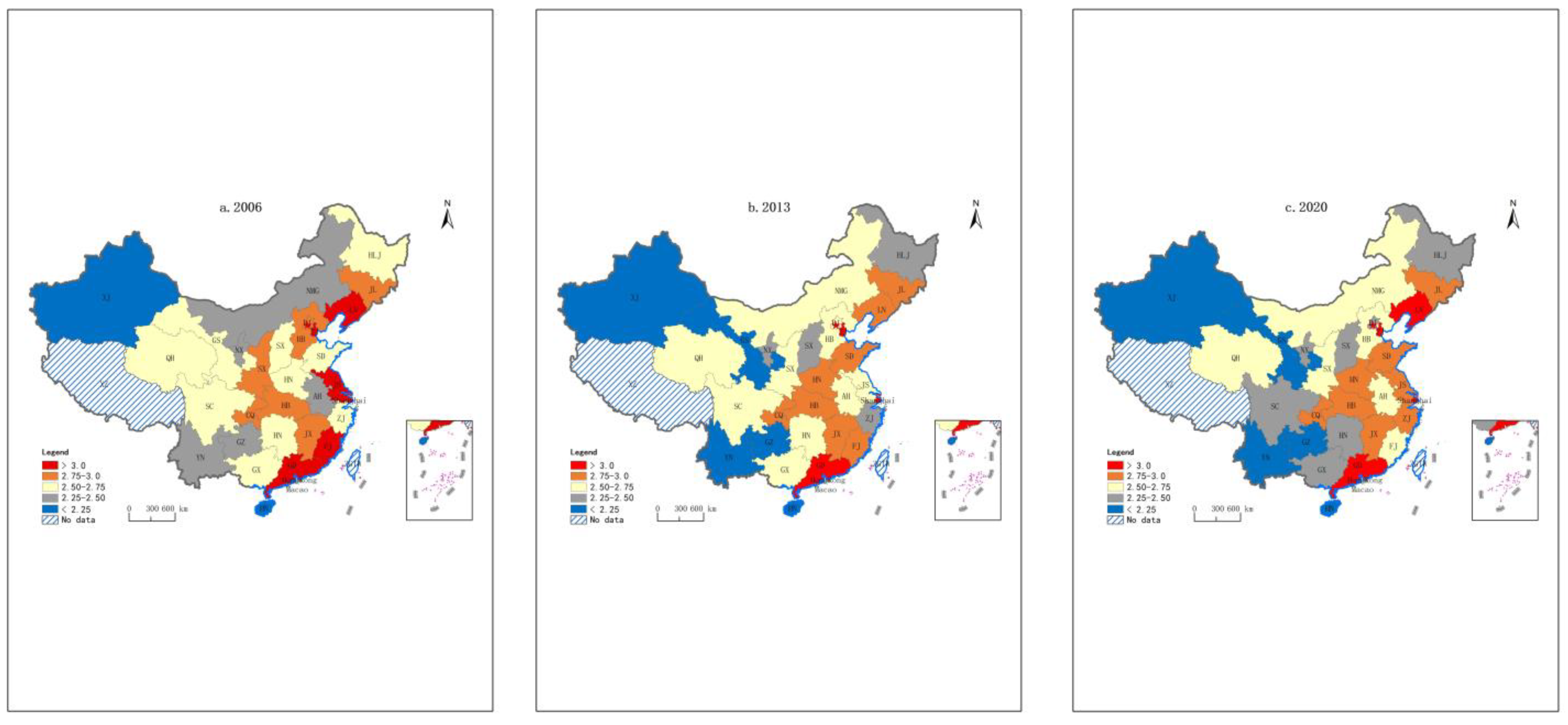
4.1.2. The Trend of LMCA Level by Region

Figure 2 shows the regional yearly trend of LMCA. The overall LMCA level is between 2.3 and 3.0 with distinct regional differences: LMCA is highest in the eastern region, and lowest in the western region, with the central region being in between. The LMCA level in the eastern region shows a gradual decreasing trend after 2012 and slightly rebounds after 2017. The LMCA level in the western region shows a slight decreasing pattern between 2.3 and 2.5, which is significantly lower than that in the other regions.

To gather further insights into the evolution of LMCA, we used the ArcGIS 10.3 software to visualize the evolution of the spatial layout of the level of LMCA at the provincial level in China for three years, namely 2006, 2013, and 2020, using the natural interruption point hierarchy method (Figure 3). The degree of co-agglomeration in the graph is represented as blue, grey, yellow, orange, and red in descending order. Figure 3 shows that there is an obvious spatial divergence in the level of co-agglomeration between the two industries in China, with a serious imbalance in the eastern, central, and western regions. Provinces with high levels of co-agglomeration (such as Tianjin, Guangdong, Shanghai, and Liaoning) are mostly located in the eastern coastal region, which has the most densely distributed transport infrastructure and the most complete and diversified industrial structure in China.

4.2. The Impact of LMCA on EcoResi

4.2.1. Analysis Results of Classical Econometric Models

An OLS regression of the panel data was first carried out in order to determine the specific form of the model. Columns 1–5 in

Table 4. OLS model estimation results for the panel data.

	(1)	(2)	(3)	(4)	(5)
Variable	OLS Mix	Individual Fixed	Time Fixed	Individual and Time Double Fixed	RE
LMCA	0.009 ***	0.036 **	0.030 ***	0.030 **	0.069 ***
	(4.12)	(2.26)	(3.44)	(2.21)	(2.76)
Intnet	−0.504 **	−0.228	−0.670 **	−0.837	−0.211
	(−2.11)	(−0.58)	(−2.13)	(−1.54)	(−0.81)
EmploDens	−0.001	0.003	−0.002 **	0.002	0.000
	(−0.85)	(1.48)	(−2.27)	(0.91)	(0.43)
HR	−0.119 ***	0.271 ***	−0.158 ***	0.111	−0.059
	(−3.27)	(2.65)	(−4.32)	(0.96)	(−1.23)
LnK	0.038 **	−0.567 ***	0.064 ***	−0.692 ***	−0.070 **
	(1.97)	(−4.89)	(3.20)	(−5.08)	(−2.33)
FDIR	−0.072	−0.215 *	0.065	−0.082	−0.013
	(−1.02)	(−1.80)	(0.87)	(−0.65)	(−1.18)
Wage	0.059 ***	0.086 ***	0.121 ***	0.071	0.016 ***
	(3.53)	(3.55)	(4.68)	(1.63)	(3.90)
Open	0.186 *	0.399 **	0.080	0.416 **	0.080
	(1.91)	(2.11)	(0.67)	(2.09)	(0.72)
Transp	0.000	0.004	−0.000	0.002	0.001
	(0.05)	(1.23)	(−0.03)	(0.70)	(0.42)
FAInv	−0.019	0.004	−0.015	0.008	0.043
	(−0.90)	(0.13)	(−0.70)	(0.26)	(1.48)
_cons	1.584 ***	2.606 *	1.390 ***	5.588 ***	2.350 ***
	(6.81)	(1.78)	(5.85)	(2.94)	(4.19)
id	No	Yes	No	Yes	No
year	No	No	Yes	Yes	No
N	450	450	450	450	450
Adj R2	0.059	0.267	0.151	0.326	0.313

Note: t-values are in parentheses. ***, **, and * indicate significance at 1%, 5%, and 10%, respectively.

show the regression results of the OLS regression, including the individual-fixed effect, time-fixed effect, individual and time double-fixed effect, and random effect. The OLS (column 1) and the time-fixed model (column 3) imply that the co-agglomeration of the two industries (LMCA) is positively correlated with regional economic resilience (EcoResi) at the significance level of 1%; the individual-fixed model (column 2) and the individual and time double-fixed model (column 4) imply that LMCA is positively correlated with EcoResi at the significance level of 5%; and the random effect of the panel data is a robust test, and its results (column 5) are consistent with the results of the other models. In summary, the co-agglomeration of the two industries (LMCA) is significantly and positively correlated with regional economic resilience (EcoResi). This indicates that the collaborative aggregation of the logistics and manufacturing industries can significantly promote regional economic resilience.

Table 5. LM test results of the spatial panel model.

LM Test	Geographical Distance Matrix		Economic Geographical Distance Matrix
	t-Value	p-Value	t-Value	p-Value
Moran’s I	3.950	0.000	4.925	0.000
LM-error	12.276	0.000	21.792	0.000
R-lmerror	3.052	0.081	12.348	0.000
LM-Lag	14.207	0.000	10.518	0.001
R-lmlag	1.122	0.290	1.073	0.300

shows the LM test results of the spatial panel model. With the geographical distance weight matrix, among the three tests for spatial error, the Moran’s index and Lagrange multiplier are significant at the 1% level; the robust Lagrange multiplier is significant at the 10% level; and the Lagrange multiplier for spatial lag is significant at 1% level. The null hypothesis of no spatial autoregression is rejected in all the tests above, indicating that the impact of LMCA on EcoResi requires spatial econometric analysis.

The Wald test and LR test were applied to the data, and the test statistics are 61.38 and 63.48, respectively, which indicate that the spatial Dubin model cannot be degenerated into spatial error or spatial autoregression model at the 1% significance level. Therefore, the spatial Dubin model (SDM) was selected for the analysis.

4.2.2. Analysis of Spatial Spillover Effects

Table 6. Regression results of geographical adjacent spatial econometric model.

	(1)	(2)	(3)	(4)
EcoResi	SDM	Weighted SDM	SLM	SEM
LMCA	0.021 ***	0.065 ***	0.004 ***	0.003 **
	(3.24)	(3.49)	(2.67)	(2.50)
Intnet	−0.081 ***	−0.160 **	−0.057 **	−0.056 **
	(−3.05)	(−2.47)	(−2.22)	(−2.17)
EmploDens	−0.000 **	−0.000	−0.000 ***	−0.000 **
	(−2.57)	(−0.26)	(−2.62)	(−2.49)
HR	−0.006 *	−0.008	−0.010 ***	−0.010 ***
	(−1.65)	(−1.09)	(−3.24)	(−2.92)
LnK	0.004 *	−0.005	0.007 ***	0.007 ***
	(1.91)	(−0.99)	(4.07)	(4.04)
FDIR	−0.002	−0.007	0.007	0.006
	(−0.33)	(−0.50)	(1.17)	(1.03)
Wage	0.010 ***	0.005	0.010 ***	0.010 ***
	(3.80)	(0.91)	(4.66)	(4.67)
Open	−0.003	0.029 *	−0.005	−0.008
	(-0.33)	(1.67)	(−0.53)	(−0.81)
Transp	0.000	−0.001 **	−0.000	−0.000
	(0.05)	(−2.47)	(−0.29)	(−0.13)
FAInv	−0.006 ***	0.005	−0.003 **	−0.004 **
	(−2.69)	(1.31)	(−1.96)	(−2.00)
Spatial:
rho	0.067	0.067	0.160 ***
	(1.09)	(1.09)	(2.72)
lambda				0.160 **
				(2.52)
Variance:
sigma2_e	0.001 ***	0.001 ***	0.001 ***	0.001 ***
	(15.24)	(15.24)	(15.21)	(15.21)
N	450	450	450	450
Adj R2	0.033	0.033	0.021	0.022

Note: t-values are in parentheses. ***, **, and * indicate significance at 1%, 5%, and 10%, respectively.

shows the estimates of the spatial econometric model of LMCA. Column 1 and column 2 of Table 6 are the estimated results of the spatial Dubin model, and the estimated coefficient of LMCA is 0.021, which is significant at 1%. Therefore, LMCA has a significant positive role in improving EcoResi. In the spatial measurement regression model with geographical weights, the estimated coefficient of LMCA is 0.065, which is significant at the level of 1%, indicating that LMCA significantly increases the spatial spillover effect of economic resilience on adjacent regions. LMCA promotes the cross-regional flow of production resources; helps industries share transportation, communication, warehousing, and other infrastructures; and saves production costs. It is conducive to the development of technological innovation and the improvement of total productivity, thus improving EcoResi. Columns (3) and (4) in Table 6 contain the regression results of the spatial lag model and the spatial error model, respectively. The regression coefficient of the LMCA level on EcoResi in both models is positive and significant at the level of 1% and 5%, respectively, which is consistent with the above analytical conclusions.

4.2.3. Analysis of Regional Spatial Spillover Effect

Table 7. Regression results of regional spatial econometric model with and without the geographical adjacent weight matrix.

	(1)	(2)	(3)	(4)
Variable	Eastern Region	Western Region	Central Region	Nationwide
LMCA	0.001	0.027 ***	0.072 **	0.021 ***
	(0.06)	(2.79)	(2.41)	(3.24)
Intnet	−0.022	−0.118 *	−0.762 ***	−0.081 ***
	(−0.50)	(−1.78)	(−4.46)	(−3.05)
EmploDens	−0.000	−0.004 *	0.000	−0.000 **
	(−0.12)	(−1.69)	(0.04)	(−2.57)
HR	−0.004	0.009	0.030 **	−0.006 *
	(−0.44)	(0.90)	(2.32)	(−1.65)
LnK	−0.007	0.006	0.069 **	0.004 *
	(−0.89)	(1.26)	(2.37)	(1.91)
FDIR	−0.015	0.078 ***	0.031	−0.002
	(−1.39)	(2.74)	(0.98)	(−0.33)
Wage	0.002	0.019 ***	−0.015	0.010 ***
	(0.59)	(3.08)	(−1.03)	(3.80)
Open	0.012	0.088	0.005	−0.003
	(0.76)	(1.41)	(0.05)	(−0.33)
Transp	−0.001 **	−0.000	0.000	0.000
	(−2.40)	(−0.87)	(0.73)	(0.05)
FAInv	0.001	−0.015 **	−0.002	−0.006 ***
	(0.27)	(−2.56)	(−0.24)	(−2.69)
Wx:
LMCA	−0.018	0.183 ***	0.068 **	0.065 ***
	(−0.65)	(3.99)	(2.46)	(3.49)
Intnet	0.063	−0.299 *	−1.312 ***	−0.160 **
	(0.70)	(−1.71)	(−5.12)	(−2.47)
EmploDens	0.000	−0.008	−0.006 ***	−0.000
	(0.80)	(−1.07)	(−2.91)	(−0.26)
HR	−0.025 **	−0.011	0.043	−0.008
	(−2.54)	(−0.44)	(1.48)	(−1.09)
LnK	0.004	−0.002	0.166 ***	−0.005
	(0.31)	(−0.27)	(2.89)	(−0.99)
FDIR	−0.013	0.036	0.044	−0.007
	(−0.81)	(0.49)	(1.13)	(−0.50)
Wage	0.005	0.035 ***	0.041 *	0.005
	(0.77)	(2.64)	(1.78)	(0.91)
Open	0.027	0.182	0.387 **	0.029 *
	(1.00)	(1.11)	(2.34)	(1.67)
Transp	−0.000	−0.001	−0.001	−0.001 **
	(−0.64)	(−1.56)	(−0.56)	(−2.47)
FAInv	−0.005	0.026	0.001	0.005
	(−0.81)	(1.53)	(0.16)	(1.31)
Spatial:
rho	−0.211 ***	−0.159	−0.148	0.067
	(−2.75)	(−1.40)	(−1.62)	(1.09)
Variance:
sigma2_e	0.001 ***	0.001 ***	0.000 ***	0.001 ***
	(8.99)	(9.45)	(7.68)	(15.24)

Note: t-values are in parentheses. ***, **, and * indicate significance at 1%, 5%, and 10%, respectively.

shows the regression results of the spatial Dubin model of the three regions and the whole country. It can be seen that without the geographical weights, the coefficient of LMCA is positive and significant at the 1% and 5% levels in both the western and central regions, indicating that LMCA significantly increases EcoResi in these regions; in the models with the geographical weights, the coefficient of LMCA is positive and significant at the 5% level in the western and central regions, indicating that LMCA has a significant spatial spillover effect on the EcoResi of adjacent regions. However, these effects are not significant in the eastern region, possibly because the eastern region is the most economically developed region of China; its logistics and manufacturing industries are sophisticated in a highly coordinated fashion, and, therefore, the impact of LMCA on EcoResi is not obvious. Open has a significant spatial spillover effect in the central region and the whole country, indicating that economic openness to the world outside of China can significantly contribute to the EcoResi of adjacent regions.

Table 8. Direct effect and spillover effect of subregional LMCA on EcoResi.

	(1)	(2)	(3)	(4)
	Eastern Region	Western Region	Central Region	Nationwide
LR_Direct:
LMCA	0.003	0.021 ***	0.068 **	0.022 ***
	(1.21)	(3.33)	(2.34)	(3.31)
Intnet	−0.031	−0.111 *	−0.680 ***	−0.085 ***
	(−0.67)	(−1.69)	(−4.10)	(−3.28)
EmploDens	−0.000	−0.003	0.001	−0.000 ***
	(−0.19)	(−1.36)	(0.42)	(−2.58)
HR	−0.001	0.009	0.028 **	−0.007 *
	(−0.15)	(0.96)	(2.19)	(−1.78)
LnK	−0.008	0.006	0.055 **	0.003 *
	(−0.94)	(1.42)	(2.13)	(1.95)
FDIR	−0.014	0.078 ***	0.029	−0.002
	(−1.28)	(2.78)	(0.97)	(−0.31)
Wage	0.002	0.018 ***	−0.017	0.010 ***
	(0.39)	(2.99)	(−1.11)	(3.73)
Open	0.009	0.080	−0.033	−0.003
	(0.57)	(1.27)	(−0.33)	(−0.33)
Transp	−0.001 **	−0.000	0.000	0.000
	(−2.34)	(−0.60)	(0.87)	(0.04)
FAInv	0.001	−0.016 ***	−0.002	−0.005 ***
	(0.39)	(−2.94)	(−0.22)	(−2.65)
LR_Indirect:
LMCA	−0.016	0.165 ***	0.055 **	0.070 ***
	(−0.65)	(3.91)	(2.29)	(3.43)
Intnet	0.064	−0.237	−1.125 ***	−0.172 **
	(0.77)	(−1.41)	(-4.33)	(−2.44)
EmploDens	0.000	−0.008	−0.006 ***	−0.000
	(0.88)	(−1.10)	(−3.04)	(−0.35)
HR	−0.022 **	−0.012	0.036	−0.009
	(−2.18)	(−0.56)	(1.26)	(−1.20)
LnK	0.004	−0.003	0.150 ***	−0.005
	(0.35)	(−0.40)	(2.95)	(−1.02)
FDIR	−0.009	0.024	0.039	−0.007
	(−0.57)	(0.35)	(1.04)	(−0.43)
Wage	0.005	0.030 **	0.041 *	0.006
	(0.77)	(2.47)	(1.84)	(1.17)
Open	0.021	0.160	0.370 **	0.029
	(0.85)	(1.10)	(2.31)	(1.52)
Transp	−0.000	−0.001	−0.001	−0.001 **
	(−0.38)	(−1.53)	(−0.76)	(−2.43)
FAInv	−0.005	0.026 *	0.002	0.005
	(−0.79)	(1.74)	(0.26)	(1.22)
LR_Total:
LMCA	−0.013	0.185 ***	0.123 ***	0.092 ***
	(−0.40)	(3.56)	(2.63)	(3.93)
Intnet	0.033	−0.347 **	−1.805 ***	−0.257 ***
	(0.40)	(−2.14)	(−5.82)	(−3.41)
EmploDens	0.000	−0.011 *	−0.005 **	−0.000
	(0.63)	(−1.77)	(−2.12)	(−1.14)
HR	−0.023 ***	−0.003	0.064 **	−0.015 **
	(−3.15)	(−0.13)	(2.11)	(−2.25)
LnK	−0.003	0.003	0.205 ***	−0.002
	(−0.28)	(0.35)	(3.15)	(−0.35)
FDIR	−0.022	0.102	0.068	−0.009
	(−1.56)	(1.37)	(1.24)	(−0.52)
Wage	0.007	0.048 ***	0.024	0.016 ***
	(1.18)	(3.30)	(1.11)	(2.79)
Open	0.031	0.240	0.337 **	0.025
	(1.20)	(1.34)	(2.56)	(1.21)
Transp	−0.001	−0.001 *	−0.000	−0.001 **
	(−1.48)	(−1.73)	(−0.21)	(−2.15)
FAInv	−0.004	0.010	0.001	−0.000
	(−0.63)	(0.58)	(0.05)	(−0.09)
N	165	165	120	450
Adj R2	0.209	0.025	0.069	0.033

Note: t-values are in parentheses. ***, **, and * indicate significance at 1%, 5%, and 10%, respectively.

shows that under the direct effect, the promotional effect and spatial spillover effect of LMCA on EcoResi are significant for the entire nation at the 1% level, but there are significant regional differences. Among them, LMCA has the strongest stimulating effect on EcoResi in the central region, followed by the western region, and it is not significant in the eastern region. For the spillover effect, the LMCA effect is significant in the western and central regions, with the coefficient of the spatial spillover effect in the western region (0.165) much higher than that in the central region (0.055), but this effect is not significant in the eastern region. The above results show that LMCA is a significant factor for promoting the EcoResi of the western and central regions and surrounding regions, while it does not exhibit a similar effect in the eastern region.

4.3. Robustness Test

To verify the above spatial measurement results and robustness, we let k and l denote two regions, and a spatial economic distance matrix was constructed using the following method [11]:

$$C_{kl}=\left(\frac{1}{|PGD{P}_l-PGD{P}_k+1|}\right)e^{-d_{kl}},$$

(7)

where $C_{kl}$ is the spatial economic distance between regions k and l; $PGD{P}_k$ and $PGD{P}_l$ denote the GDP per capita of regions k and l, respectively; and $d_{kl}$ denotes the geographical distance between the administrative centers of regions k and l.

Table 9. Regression results of subregional spatial econometric models under economic geographical weight matrix.

	(1)	(2)	(3)	(4)
	Eastern Region	Western Region	Western Region	Nationwide
LMCA	0.014	0.022 **	0.089 ***	0.026 **
	(0.93)	(2.01)	(3.15)	(2.15)
Intnet	−0.009	−0.124 **	−0.261 *	−0.030
	(−0.18)	(−2.16)	(−1.73)	(−0.98)
EmploDens	−0.000	0.004 ***	0.001	−0.000
	(−0.95)	(2.62)	(0.81)	(−0.81)
HR	−0.021 **	0.015 *	−0.008	−0.008 **
	(−2.23)	(1.82)	(−0.49)	(−2.46)
LnK	−0.017 **	−0.006	0.055 *	−0.009 **
	(−2.43)	(−0.77)	(1.70)	(−2.21)
FDIR	−0.002	0.045 *	0.039	0.009
	(−0.17)	(1.90)	(1.05)	(1.28)
Wage	0.007	0.006	0.023	0.007 **
	(1.38)	(0.84)	(1.27)	(2.49)
Open	0.006	−0.135 ***	0.195	−0.010
	(0.40)	(−3.00)	(1.15)	(−0.85)
Transp	−0.001	−0.001 ***	0.001	0.000
	(−1.47)	(−3.09)	(1.11)	(0.17)
FAInv	0.003	−0.001	−0.020 ***	0.004 *
	(0.99)	(−0.15)	(−2.72)	(1.76)
Wx:
LMCA	0.019	0.043 **	0.013 **	0.019 ***
	(0.59)	(2.10)	(2.25)	(3.02)
Intnet	−0.009	0.425 **	0.071	−0.168 ***
	(−0.06)	(2.14)	(0.20)	(−3.15)
EmploDens	−0.000	0.002	0.007 **	0.000
	(−0.82)	(0.33)	(2.00)	(1.07)
HR	−0.024	−0.014	0.003	0.002
	(−1.64)	(−0.74)	(0.09)	(0.30)
LnK	−0.012	0.013	0.068	0.002
	(−0.36)	(0.83)	(1.07)	(0.17)
FDIR	−0.011	0.002	0.021	0.048 **
	(−0.31)	(0.03)	(0.40)	(2.46)
Wage	0.019	−0.024	0.047	−0.009
	(1.51)	(−1.31)	(1.12)	(−1.36)
Open	0.058	0.157	0.240	−0.004
	(1.30)	(1.13)	(1.10)	(−0.15)
Transp	0.002 **	−0.000	−0.001	0.000
	(2.34)	(−0.22)	(−0.74)	(0.85)
FAInv	−0.005	−0.026 *	−0.008	0.006
	(−0.69)	(−1.75)	(−0.55)	(1.00)
Spatial:
rho	0.023	0.128	0.221 **	0.012
	(0.21)	(1.12)	(1.98)	(0.14)
Variance:
sigma2_e	0.001 ***	0.000 ***	0.001 ***	0.001 ***
	(9.08)	(9.06)	(7.66)	(15.00)
N	165	165	120	450
Adj R2	0.045	0.216	0.161	0.034

Note: t-values are in parentheses. ***, **, and * indicate significance at 1%, 5%, and 10%, respectively.

shows the spatial Durbin model regression results with and without the economic geographical weight matrix in the eastern, western, and central regions, and the whole country. It can be seen that without the geographical weights, the regression coefficients of LMCA are positive and significant at the 5%, 1%, and 5% level in the western region, the central region, and nationwide, respectively. When weighted by the geographical weights, the regression coefficients of LMCA are positive and significant at the 1% significance level for the entire country and at the 5% level in the western and central regions, indicating that LMCA has a significant spatial spillover promotion effect on the EcoResi of neighboring regions; however, once again, we notice that the promotional effect and the spatial spillover effect are not significant in the eastern region. This is consistent with the results of the spatial econometric regression of geographical adjacent weights in Table 5, which verifies the robustness of the spatial spillover effect of LMCA on EcoResi.

4.4. Discussion

This study shows that LMCA can enhance EcoResi through synergistic and spillover effects, but the impact of LMCA on EcoResi is heterogeneous in regions where spatial heterogeneity exists. Our empirical results indicate that cooperative effects based on industry linkages accelerate the free flow of production factors, improve the efficiency of resource utilization, form economies of scale, and promote regional innovation, thus improving EcoResi. EcoResi is influenced by a variety of factors, such as natural resource endowments, industrial structure, policy regimes, and cultural practices.

The research findings contribute to the development of regional integration. First, the logistics service industry has unique characteristics from other service industries. It is the productive service industry most closely related to the manufacturing industry, forming linkages between the upstream and downstream of a supply chain. LMCA is of practical significance in reducing logistic costs, improving service quality, and achieving high-quality, integrated, and coordinated development of a regional economy [37,56]. This study explores the spatial correlation and spatial spillover effects of LMCA from the perspective of enhancing EcoResi and finds that the spatial heterogeneity of collaboration and the trade-off between various cooperative effects can improve EcoResi. Secondly, the findings show that the degree of LMCA in the eastern region of China is higher than that in the central and western regions, but the contribution of LMCA to EcoResi is not significant in the eastern region. China’s manufacturing industry is in the middle-and-low end of the global value chain, and the high concentration of industries in the eastern region brings about a crowding effect due to resource scarcity, and LMCA generates negative externalities [57]. Through the spillover effect of LMCA, the eastern region opens up new industrial layout space to the central and western regions in the mode of industrial gradient transfer. In turn, through the deepening of intra-industry division of labor and technological advancement, the region itself extends to the middle-and-high end of the manufacturing value chain to achieve industrial transformation and upgrading [42,58,59], bringing into play the positive externalities of co-agglomeration.

The above findings suggest the following: First, the spatial co-agglomeration of the logistics and manufacturing industries should be promoted to enhance regional economic resilience. The Chinese government should play an active role in this effort by applying regulatory and economic tools at its disposal [7,37,48], including the following: (1) provide enterprises with sound infrastructure, such as transportation, energy, education, and medical care, enhance the region’s ability to take on external industrial transfers, and create a good working and living environment; (2) improve the level of logistics outsourcing in the manufacturing industry, expand the market demand for third-party logistics services, promote the innovation of logistics services to reduce logistics costs, and lay a solid material foundation for the co-agglomeration of logistics and manufacturing; (3) enable the service industry to play a more significant role in integrating innovation factors and improving independent innovation capacity by building public service platforms, such as financing and collaborative innovations; (4) provide a fair and just environment for entrepreneurship and market transactions, as well as systematic legal protection for the coordinated management of enterprises in the agglomeration area; and (5) respect the laws of regional economic development, ensure the effective supply of resources by the market while avoiding mismatches, and provide sound financial and taxation support to guide the collaborative spatial agglomeration of industries and promote industrial transformation and upgrading.

Secondly, the regional difference in economic development level is correctly recognized, with developed regions playing a role of radiation and demonstration to build and share resources, and relatively under-developed regions actively seeking connectivity with their neighbors. Exerting the macro-regulatory role of the state, implementing a regional integrated development strategy, promoting the co-agglomeration of the logistics and manufacturing industries, and successfully improving the overall economic resilience of local regions are important [60,61].

This topic discussed in this paper can be extended in a few directions. For example, some factors that may have significant effects on regional economic resilience, such as business environment and local culture, are not considered in this paper because of the lack of reliable measures. In the future, the data can be expanded by developing appropriate measures to quantify these factors using other methods, such as field study with questionnaire surveys and experimental research methods. With reliable quantitative measures of these factors, the current research can be further improved. In addition, this study only focuses on the co-agglomeration of the logistics and manufacturing industries and the regional economic resilience of 30 provinces in mainland China, which is a limited sample, and future research can pave the road for expanding the regional coverage.

5. Conclusions

Facing a severe external environment, such as the global COVID-19 pandemic and frequent natural disasters in recent years, it is imperative to improve regional economic resilience. This paper analyzes the influence mechanism and spatial spillover effects of the co-agglomeration between the logistics and manufacturing industries on regional economic resilience from the perspectives of theoretical analysis and empirical test based on the provincial panel data of 30 provinces in mainland China from 2006 to 2020. The main findings of this paper are as follows: First, the degree of co-agglomeration between the logistics and manufacturing industries is highest in the eastern region and lowest in the western region. The degree of co-agglomeration in both regions decreases over time. In between is the central region, with an increasing trend in the degree of co-aggregation. Regional economic resilience fluctuates the least in the eastern region, while it oscillates significantly in the central region. Secondly, the regression analysis results show that the increase in co-agglomeration between the two industries not only improves local economic resilience but also has a significant spatial spillover effect. The regional regression results show that the promotional and spatial spillover effects differ by region. More specifically, the effects are significant in the central and western regions, but the effects are not significant in the eastern region. This may be due to the highly developed economy in this region, where the logistics and manufacturing industries are already well developed in a highly collaborative fashion. Therefore, its economic resilience is not sensitive to the change (or lack thereof) in LMCA. This study enriches the literature on the effect of co-agglomeration of the two industries on regional economic resilience from the perspectives of industrial association and synergy as well as spatial spillover, which provides decision-making references for the country’s industrial spatial layout, industrial structure transformation and upgrading, and improvement of macroeconomic regulation and control policies.

References

1. Yan, R. Research on the collaborative development of modern logistics and manufacturing under the new development pattern: Micro-site behavior analysis based on enterprises in big cities. Guizhou Soc. Sci. 2021, 382, 135–144. [Google Scholar]
2. Zhao, C.Y.; Wang, S.P. The impact of economic agglomeration on the economic resilience of cities. J. Zhongnan Univ. Econ. Law 2021, 1, 102–114. [Google Scholar]
3. Kitsos, A.; Carrascal-Incera, A.; Ortega-Argilés, R. The role of embeddedness on regional economic resilience: Evidence from the UK. Sustainability 2019, 11, 3800. [Google Scholar] [CrossRef]
4. Li, L.; Zhang, P.; Tan, J.; Guan, H. Review on the evolution of resilience concept and research progress on regional economic resilience. Hum. Geogr. 2019, 34, 1–7+151. [Google Scholar] [CrossRef]
5. Brown, L.; Greenbaum, R.T. The role of industrial diversity in economic resilience: An empirical examination across 35 Years. Urban Stud. 2017, 54, 1347–1366. [Google Scholar] [CrossRef]
6. Rocchetta, S.; Mina, A. Technological coherence and the adaptive resilience of regional economies. Reg. Stud. 2019, 53, 1421–1434. [Google Scholar] [CrossRef]
7. Yan, F.; Wang, T. Professional agglomeration, collaborative agglomeration and regional economic growth of logistics and manufacturing industries. Enterp. Econ. 2021, 4, 88–97. [Google Scholar] [CrossRef]
8. Feng, Y.; Lee, C.C.; Peng, D.Y. Does regional integration improve economic resilience? Evidence from urban agglomerations in China. Sustain. Cities Soc. 2023, 88, 104273. [Google Scholar] [CrossRef]
9. Chen, Y.W.; Wu, W.K. Research on the relationship between industrial agglomeration, industrial diversification and urban economic resilience. Sci. Technol. Prog. Policy 2021, 38, 64–73. [Google Scholar]
10. Wang, Z.X.; Wei, W. Regional economic resilience in China: Measurement and determinants. Reg. Stud. 2021, 55, 1228–1239. [Google Scholar] [CrossRef]
11. Zhang, W.; Hu, Y. The effect of innovative human capital on green total factor productivity in the Yangtze River Delta: An empirical analysis based on the spatial Durbin model. China Popul. Resour. Environ. 2020, 30, 106–120. [Google Scholar] [CrossRef]
12. Reggiani, A.; De Graaff, T.; Nijkamp, P. Resilience: An evolutionary approach to spatial economic systems. Netw. Spat. Econ. 2002, 2, 211–229. [Google Scholar] [CrossRef]
13. Simmie, J. The economic resilience of regions: Towards an evolutionary approach. Camb. J. Reg. Econ. Soc. 2009, 3, 27–43. [Google Scholar] [CrossRef]
14. Martin, R.; Sunley, P. On the notion of regional economic resilience: Conceptualization and explanation. J. Econ. Geogr. 2015, 15, 1–42. [Google Scholar] [CrossRef]
15. Xu, Y.; Warner, M. Understanding employment growth in the recession: The geographic diversity of state rescaling. Camb. J. Reg. Econ. Soc. 2015, 8, 359. [Google Scholar] [CrossRef]
16. Adger, W.N. Social capital, collective action, and adaptation to climate change. Econ. Geogr. 2009, 79, 327–345. [Google Scholar] [CrossRef]
17. Hauser, C.; Tappeiner, G.; Walde, J. The learning region: The impact of social capital and weak ties on innovation. Reg. Stud. 2007, 41, 75–88. [Google Scholar] [CrossRef]
18. Quan, T.; Quan, T. A Study of the Spatial Mechanism of Financial Agglomeration Affecting Green Low-Carbon Development: Evidence from China. Sustainability 2023, 15, 965. [Google Scholar] [CrossRef]
19. Martin, R. Regional economic resilience, hysteresis and recessionary shocks. J. Econ. Geogr. 2012, 12, 1–32. [Google Scholar] [CrossRef]
20. Whitley, R. The institutional structuring of innovation strategies: Business systems, firm types and patterns of technical change in different market economies. Organ. Stud.-ORGAN STUD 2000, 21, 855–886. [Google Scholar] [CrossRef]
21. Huggins, R.; Thompson, P. Local entrepreneurial resilience and culture: The role of social values in fostering economic recovery. Camb. J. Reg. Econ. Soc. 2015, 8, 313–330. [Google Scholar] [CrossRef]
22. Chi, Y.; Fang, Y.H.; Liu, J. Spatial–temporal evolution characteristics and economic effects of China’s cultural and tourism industries’ collaborative agglomeration. Sustainability 2022, 14, 15119. [Google Scholar] [CrossRef]
23. Tan, J.; Hu, X.; Hassink, R.; Ni, J. Industrial structure or agency: What affects regional economic resilience? Evidence from resource-based cities in China. Cities 2020, 106, 102906. [Google Scholar] [CrossRef]
24. Duan, W.; Madasi, J.D.; Khurshid, A.; Ma, D. Industrial structure conditions economic resilience. Technol. Forecast. Soc. Chang. 2022, 183, 121944. [Google Scholar] [CrossRef]
25. Peng, R.; Liu, T.; Cao, G. Spatial pattern of urban economic resilience in eastern coastal China and industrial explanation. Geogr. Res. 2021, 40, 1732–1748. [Google Scholar] [CrossRef]
26. Petrakos, G.; Psycharis, Y. The spatial aspects of economic crisis in Greece. Camb. J. Reg. Econ. Soc. 2015, 9, 137–152. [Google Scholar] [CrossRef]
27. Doran, J.; Fingleton, B. US Metropolitan Area Resilience: Insights from dynamic spatial panel estimation. Environ. Plan. A Econ. Space 2017, 50, 111–132. [Google Scholar] [CrossRef]
28. Xu, Y.; Wang, C. Influencing factors of regional economic resilience in the 2008 financial crisis: A case study of Zhejiang and Jiangsu Provinces. Prog. Geogr. 2017, 36, 986–994. [Google Scholar] [CrossRef]
29. Sun, J.; Sun, X. Research progress of regional economic resilience and exploration of its application in China. Geogr. Res. 2017, 37, 1–9. [Google Scholar] [CrossRef]
30. Davies, S. Regional resilience in the 2008–2010 downturn: Comparative evidence from European countries. Camb. J. Reg. Econ. Soc. 2011, 4, 369–382. [Google Scholar] [CrossRef]
31. Hirschman, A. On the Strategy of Economic Development; Yale University Press: New Haven, CT, USA, 1958. [Google Scholar]
32. Bergman, E.M.; Feser, E.J. Industrial and Regional Clusters: Concepts and Comparative Applications; West Virginal University Press: Morgantown, WV, USA, 1999; Available online: https://researchrepository.wvu.edu/rri-web-book/5/ (accessed on 6 August 2022).
33. Li, G.; Jin, F.; Chen, Y.; Jiao, J.; Liu, S. Location characteristics and differentiation mechanism of logistics industry based on points of interest: A case study of Beijing. Acta Geogr. Sin. 2017, 72, 1091–1103. [Google Scholar] [CrossRef]
34. Perroux, F. Economic space: Theory and applications. Q. J. Econ. 1950, 64, 89–104. [Google Scholar] [CrossRef]
35. Chen, X.; Chen, Z. Level and effect on co-agglomeration of producer service and manufacturing industry: Empirical evidence from the eastern area of China. Financ. Trade Res. 2014, 25, 49–57. [Google Scholar]
36. Zeng, W.; Li, L.; Huang, Y. Industrial collaborative agglomeration, marketization, and green innovation: Evidence from China’s provincial panel data. J. Clean. Prod. 2021, 279, 123598. [Google Scholar] [CrossRef]
37. Liu, M. The Influence of Collaborative Agglomeration of Logistics Industry and Manufacturing Industry on High-quality Economic Development: The Empirical Research on 283 Cities at the Prefecture Level and Above. China Bus. Mark. 2021, 35, 22–31. [Google Scholar] [CrossRef]
38. Dou, J.; Liu, Y. Can Co-agglomeration between producer services and manufactures promote the urban economic growth? Based on the panel data of China’s 285 cities. Mod. Financ. Econ.-J. Tianjin Univ. Financ. Econ. 2016, 315, 92–102. [Google Scholar]
39. Chen, G.; Chen, J. Industrial correlation, spatial geography and co-agglomeration of secondary and tertiary industries: Experience investigation from 212 cities in China. Manag. World 2012, 4, 82–100. [Google Scholar]
40. Ke, S.; He, M.; Yuan, C. Synergy and co-agglomeration of producer services and manufacturing: A panel data analysis of Chinese cities. Reg. Stud. J. Reg. Stud. Assoc. 2014, 48, 1829–1841. [Google Scholar] [CrossRef]
41. Yuan, Y.; Gao, K. The synergetic agglomeration of industries, spatial knowledge spillovers and regional innovation efficiency. Stud. Sci. Sci. 2020, 38, 1966–1975+2007. [Google Scholar] [CrossRef]
42. Zhang, H.; Han, A.; Yang, Q. Spatial effect analysis of synergetic agglomeration of manufacturing and producer services in China. J. Quant. Tech. Econ. 2017, 34, 3–20. [Google Scholar]
43. Briguglio, L.; Cordina, G.; Farrugia, N.; Vella, S. Economic vulnerability and resilience: Concepts and measurements. Oxf. Dev. Stud. 2009, 37, 229–247. [Google Scholar] [CrossRef]
44. Wang, S.P.; Zhao, C.Y. City resilience and city exports: An empirical study based on panel data of Chinese city. J. Shanxi Univ. Financ. Econ. 2016, 38, 1–14. [Google Scholar] [CrossRef]
45. Faggian, A.; Gemmiti, R.; Jaquet, T.; Santini, I. Regional economic resilience: The experience of the Italian local labor systems. Ann. Reg. Sci. 2018, 60, 393–410. [Google Scholar] [CrossRef]
46. Ellison, G.; Glaeser, E.L. Geographic concentration in us manufacturing industries: A dartboard approach. J. Political Econ. 1997, 105, 889–927. [Google Scholar] [CrossRef]
47. Ellison, G.; Glaeser, E.L.; Kerr, W. What causes industry agglomeration? Evidence from co-agglomeration patterns. Am. Econ. Rev. 2010, 100, 1195–1213. [Google Scholar] [CrossRef]
48. Tang, C.; Qiu, J.; Zhang, L.; Li, H. Spatial econometric analysis on the influence of elements flow and industrial collaborative agglomeration on regional economic growth: Based on manufacturing and producer services. Econ. Geogr. 2021, 41, 146–154. [Google Scholar] [CrossRef]
49. Han, Y.; Wu, L. Disentangling FDI innovation spillovers to Chinese agricultural firms: A threshold regression analysis based on absorptive capacity. J. Int. Trade 2020, 8, 132–146. [Google Scholar] [CrossRef]
50. Central Committee of the Communist Party of China. Communiqué of the Third Plenary Session of the Eleventh Central Committee (1978); Xinhua News Agency: Beijing, China, 2009.
51. Liu, B.; Lin, T. The theoretical and empirical study of the relationship between logistics outsourcing and productivity of manufacturing industry. China Ind. Econ. 2010, 9, 67–77. [Google Scholar]
52. Young, A. Gold into base metals: Productivity growth in the People’s Republic of China during the reform period. J. Political Econ. 2003, 111, 1220–1261. [Google Scholar] [CrossRef]
53. Zhang, J.; Wu, G.; Zhang, J. The Estimation of China’s provincial capital stock: 1952–2000. Econ. Res. J. 2004, 10, 35–44. [Google Scholar]
54. Myrdal, G. Myrdal, G. Economic Theory and Underdeveloped Regions; Gerald Duckworth & Co. Ltd.: London, UK, 1957. [Google Scholar]
55. Zhang, Z.; Zhao, R.Y. Research on the spatial spillover effect of financial industry agglomeration on regional economic resilience. Contemp. Econ. Manag. 2021, 43, 89–97. [Google Scholar] [CrossRef]
56. Wang, J.; Deng, Y.Z.; Kumari, S.; Song, Z. Research on the Spatial Spillover Effect of Transportation Infrastructure on Urban Resilience in Three Major Urban Agglomerations in China. Sustainability 2023, 15, 5543. [Google Scholar] [CrossRef]
57. Williamson, J.G. Regional inequality and the process of national development: A description of patterns. Econ. Dev. Cult. Change 1965, 13, 3–45. [Google Scholar] [CrossRef]
58. Li, G.Z.; Liu, M.C. Spatiotemporal evolution and influencing factors of economic resilience: Evidence from resource-based cities in China. Sustainability 2022, 14, 10434. [Google Scholar] [CrossRef]
59. Friedmann, J. Regional Development Policy: A Case Study of Venezuela; MIT Press: Cambridge, MA, USA, 1966. [Google Scholar]
60. Ren, C.Q.; Sun, D.Q.; Zhai, G.F.; Li, Y. A comprehensive assessment and spatial difference of China’s provincial economic vulnerability. Econ. Geogr. 2019, 39, 37–46. [Google Scholar] [CrossRef]
61. Wang, X.L.; Wang, L. Research on the industrial upgrading effect and regional differences of China’s logistics industry and manufacturing industry integration development on manufacturing industry. Inq. Into Econ. Issues 2022, 2, 94–111. [Google Scholar]
Figure 1. Yearly EcoResi in China’s three major economic regions.
Sustainability 15 08208 g001
Figure 2. Yearly LMCA level in China’s three major economic regions.
Sustainability 15 08208 g002
Figure 3. Yearly LMCA level by province in China. Note: The map is based on the standard map with the review number GS (2020) 4632 downloaded from the standard map service website of the Map Technical Review Centre of the Ministry of Natural Resources.
Sustainability 15 08208 g003