Optimal Parking Path Planning and Parking Space Selection Based on the Entropy Power Method and Bayesian Network: A Case Study in an Indoor Parking Lot

Abstract

According to the vehicle dynamics model and the requirements of reliable safety and minimal time, the path planning problem of parking in different types of parking spaces is solved by obstacle avoidance analysis and motion analysis in the case of the optimal solution, and the parking trajectory from the initial position to the designated parking space is obtained. In the static situation, different parking spaces in the parking space are occupied; analyze the parking space type, parking space left and right occupancy situation, and the distance between the vacant parking space and the starting point location of unoccupied cars; and establish the attribute information matrix R₀ of the vacant parking space and calculate the KMO value of the matrix R₀. This is completed to determine the weak correlation between the attributes of the vacant parking space and use the matrix R₀ as the original evaluation matrix of the entropy weight method, using the entropy weight method to calculate the three attributes of parking space type, parking space left and right occupancy situation, and distance between starting point and parking space. These results are weighted in the optimal parking space selection process, the difficulty score of the vacant parking space is determined, and the optimal parking space is determined through the ranking of the scores. In the dynamic case, the number of parking spaces and parking space usage will change over time, with the help of the Bayesian network, the existing parking spaces and number of spaces in the parking lot at the previous moment are learned according to the computer clock, which can be used to reason about the number of parking spaces and parking space availability in the parking lot at the next moment. The weights of the three attributes of parking space type, parking space left and right situation, and distance between the starting point and parking space are updated in the case of a dynamic change of parking space, and then the parking difficulty score of a new vacant parking space using the entropy weight method is used to select the optimal parking space in the dynamic situation. The optimized parking path planning and parking space selection method could contribute to enhancing parking efficiency for the sustainable management of indoor parking lots.

1. Introduction

Over the decades, with the rapid development of economics, personal vehicles have gradually entered a large number of households, becoming the first choice for traveling. With the increasing scale of car ownership in China, the contradiction between the supply and demand of cars and parking spaces in the city is getting bigger and bigger, and the problem of difficulty parking in public parking lots has become particularly prominent.

The difficulty of “parking” comes from two main sources: (1) it is not easy to choose the right parking space, and (2) there is a certain technical difficulty in parking operation. With the limited parking space, the driver’s line of sight is obstructed, and it is difficult to quickly and easily find the optimal parking space. The small parking space makes parking a more complex task. In general, drivers park with the assistance of the backup radar, backup camera, etc., but these assists still have limitations. The car may still be in the parking process and two cars scraping or collision with pedestrians can occur. Indoor parking-assisted parking technology has strong practical significance, which can provide practical convenience for human beings; shorten the time required for vehicle parking; significantly improve the safety, stability, and convenience of the parking process; improve the accuracy of vehicle perception of the environment; make the vehicle park accurately into the target parking space; and greatly reduce the risk caused by improper operation, insufficient technology, and emotional and psychological instability of the driver from the operational level; thus, it has broad research prospects and practical significance for project implementation.

Lee [1] et al. proposed an HDL-32E LIDAR automatic parking method based on self-driving cars by improving the random tree (RRT) algorithm for rapid exploration and using a fuzzy logic controller to control the brake and gas pedal for speed stabilization. Zhang [2] et al. built an environment model close to the actual environment, and then constructed a reward function to evaluate and filter the parking data. Finally, a reinforcement learning-based automatic parking method is proposed by using neural networks to learn parking strategies from the filtered data. Gan [3] et al. improved the a-star algorithm by using RS curves and potential functions; introduced an NMPC trajectory optimizer based on vehicle kinematic constraints, minimum deviation objective, and obstacle avoidance objective; and proposed a spatiotemporal heuristic method. Zhang [4] et al. first calibrated the vehicle position, obstacles, and parking spaces, and then generated the kinematic space constraints and proposed a shortest parking path generation strategy for an automatic parking system based on a bidirectional width first-search algorithm and an improved Bellman–Ford algorithm. Su [5] et al. proposed a secondary parallel automatic parking method of endpoint regionalization, and then designed a reasonable parking terminal area, planned a secondary parallel parking path, established a parking path function with constraints, and used a genetic algorithm to optimize the parking path function as the objective function; the design result is 4.1% shorter than the original path. García [6] et al. provided a solution that is based on the analysis of zenith images using artificial vision, and the solution can not only detect whether there are vehicles in the parking space, but also use the region-based convolutional neural network to detect the area occupied by the parking space, with an accuracy rate of 98.21%; finally, the appropriate parking space is specified for the vehicle. Oetiker [7] et al. proposed a closed-loop method to solve the semi-autonomous non-holonomic vehicle parking assistance method. The method allowed for a priori unknown and potential high speed and dynamic environment changes; at the same time, the computational cost of the storage efficient algorithm was very low, and it could well perceive the surrounding environment and adapt, thus gradually improving parking safety. Zhang [8] et al. proposed a DWT-Bi-LSTM parking space availability prediction model based on historical parking data: first, the threshold method was used to process the sequence data; then, the model learned from the historical denoising data to effectively avoid errors; finally, the forward and backward LSTM further improved the prediction accuracy, and the prediction speed was quicker. Peng [9] et al. proposed a new c-non-holonomic trajectory method: first, by defining the c-nonholonomic configuration, the c-non-holonomic trajectory was obtained; second, the Lyapunov method was used to demonstrate the convergence of the globally discontinuous time-invariant feedback controller; finally, the motion trajectory during parking was analyzed.

Although the research [10,11,12,13,14,15] on assisted parking technology is mostly concentrated in the field of unmanned driving, unmanned vehicles will not be widely popularized in the next decade, so it is more desirable to introduce some small and intelligent algorithms into public life to help them have a faster, better, and safer experience in the daily parking process.

This paper presents a fast-assisted parking method based on the entropy power method and Bayesian network for optimal parking spot selection and path planning for an optimized parking lot operation. The vehicle kinematic model and parking plot were established for analyzing the optimum parking path within a common parking condition, the different directions of the parking path, and the locations of parking spaces. Both the static and dynamic conditions were studied and analyzed based on the proposed models. The results represented an efficient method for parking path guidance and parking space selection, which could be applied in parking lot arrangements for fast and safe parking. With improved parking efficiency, the sustainable management of indoor parking lots could be better facilitated in the future application.

2. Methods and Model Establishment

2.1. Vehicle Model

2.1.1. Vehicle Parameters

The vehicle parameters are as follows: body length of 4.9 m and width of 1.8 m; car wheelbase of 2.8 m and wheel spacing of 1.7 m; maximum acceleration of 3.0 m/s, maximum deceleration limit of −6.0 m/s², and acceleration of no more than 20.0 m/s³; steering wheel maximum angle of 470°, steering wheel and front wheel angle of transmission ratio of 16:1 (steering wheel rotation 16°), maximum steering wheel rotation angle of 470°, ratio of the steering wheel to front wheel rotation of 16:1 (steering wheel rotation 16°, front wheel rotation 1°), and maximum speed of the steering wheel of 400°/s.

2.1.2. Vehicle Kinematic Model

Firstly, the vehicle solid model is simplified into a two-dimensional plane kinematics model, as shown in Figure 1. The points $A\left(x_A,y_A\right)$, $B\left(x_B,y_B\right)$, $C\left(x_C,y_C\right)$, and $D\left(x_D,y_D\right)$ in Figure 1 represent the left front vertex, right front vertex, right rear vertex, and left rear vertex of the vehicle, respectively; $b\left(x_b,y_b\right)$, $c\left(x_c,y_c\right)$, and $d\left(x_d,y_d\right)$ represent the contact points between the left front wheel, right front wheel, right rear wheel, and left rear wheel of the vehicle and the ground, respectively; $\left(x_f,y_f\right)$ and $\left(x_r,y_r\right)$ represent the center point coordinates of the front axis and the center point coordinates of the rear axis of the vehicle, respectively; $v_f$ and $v_r$ represent the center point velocities of the front axis and the rear axis, respectively. $l$ $L$ indicates the length of the vehicle body, $d$ indicates the width of the vehicle body, ${\delta }_i$ and ${\delta }_o$ respectively indicate the Ackermann angle of the left front wheel and the right front wheel of the vehicle, $\phi$ indicates the equivalent Ackermann angle of the two front wheels, and $\theta$ indicates the heading angle of the vehicle.

From Figure 1, it can be seen that there is a geometric relationship between the front axle center point $\left(x_f,y_f\right)$ and the rear axle center point $\left(x_r,y_r\right)$ of the vehicle, as shown in Equation (2).

$$\{\begin{array}{l}{x}_r=x_f-l\cdot \cos \theta \\ y_r=x_f-l\cdot \cos \theta \end{array}$$

(1)

The differentiation of Equation (2) yields

$$\{\begin{array}{l}{\dot{x}}_r={\dot{x}}_f+\dot{\theta }\cdot l\cdot \sin \theta \\ {\dot{y}}_r={\dot{y}}_f-\dot{\theta }\cdot l\cdot \cos \theta \end{array}$$

(2)

In the process of parking the vehicle, considering the safety issue, the vehicle is considered to be in a low-speed motion, at which time the lateral force of the rear wheels of the vehicle is ignored, and cases such as sideslip and sideswipe are not considered. Therefore, the velocity of the rear wheels of the vehicle in the axial direction is 0, and thus the velocity component of the velocity of the rear axle center point in the x-axis and y-axis directions has a certain geometric relationship, as shown in Equation (4).

$$v_{rx}\cdot \sin \theta =v_{ry}\cdot \cos \theta$$

(3)

That is, there exists a geometric relationship between the horizontal and vertical coordinates of the center point of the rear axis, as shown in Equation (5).

$${\dot{x}}_r\cdot \sin \theta ={\dot{y}}_r\cdot \cos \theta$$

(4)

There is a geometric relationship between the velocity components of the vehicle forward circumference center point velocity $v_f$ in the $x$ and $y$ axes, as shown in Equation (6).

$$\{\begin{array}{l}{v}_{fx}=v_f\cdot \cos \left(\theta +\phi \right)\\ v_{fy}=v_f\cdot \sin \left(\theta +\phi \right)\end{array}$$

(5)

That is, the relationship between the horizontal and vertical coordinates of the center point of the front axis and its velocity can be expressed as

$$\{\begin{array}{l}{\dot{x}}_f=v_f\cdot \cos \left(\theta +\phi \right)\\ {\dot{y}}_f=v_f\cdot \sin \left(\theta +\phi \right)\end{array}$$

(6)

Combining Equations (3), (5), and (7) yields the angular velocity of the vehicle heading as

$$\dot{\theta }=\frac{v_f\cdot \sin \phi }{l}$$

(7)

Equations (7) and (8) represent the geometric relationship that exists between the velocity components of the center point of the rear axis at $x$ and $y$ axes, as shown in Equation (9).

$$\{\begin{array}{l}{\dot{x}}_r=v_f\cdot \cos \theta \cdot \cos \phi \\ {\dot{y}}_r=v_f\cdot \sin \theta \cdot \cos \phi \end{array}$$

(8)

There is a geometric relationship between the front axle centroid velocity and the rear axle centroid velocity of the vehicle, as shown in Equation (10).

$$v_r=v_f\cdot \cos \phi$$

(9)

Normally, the front wheels mainly control the direction of the vehicle movement, and the rear wheels provide power to determine the running speed of the vehicle; therefore, in the process of the low-speed motion of the vehicle parking, the overall motion speed of the vehicle is replaced by the speed of the center point of the rear axle of the vehicle, which is noted as $v$, and the center point of the rear perimeter of the vehicle is taken as the reference point of the vehicle motion; then, the equation of motion state of the center point of the rear axle of the vehicle can be expressed as

$$\{\begin{array}{l}{\dot{x}}_r=v\cdot \cos \theta \\ {\dot{y}}_r=v\cdot \sin \theta \\ \dot{\theta }=\frac{v\cdot \tan \phi }{l}\end{array}$$

(10)

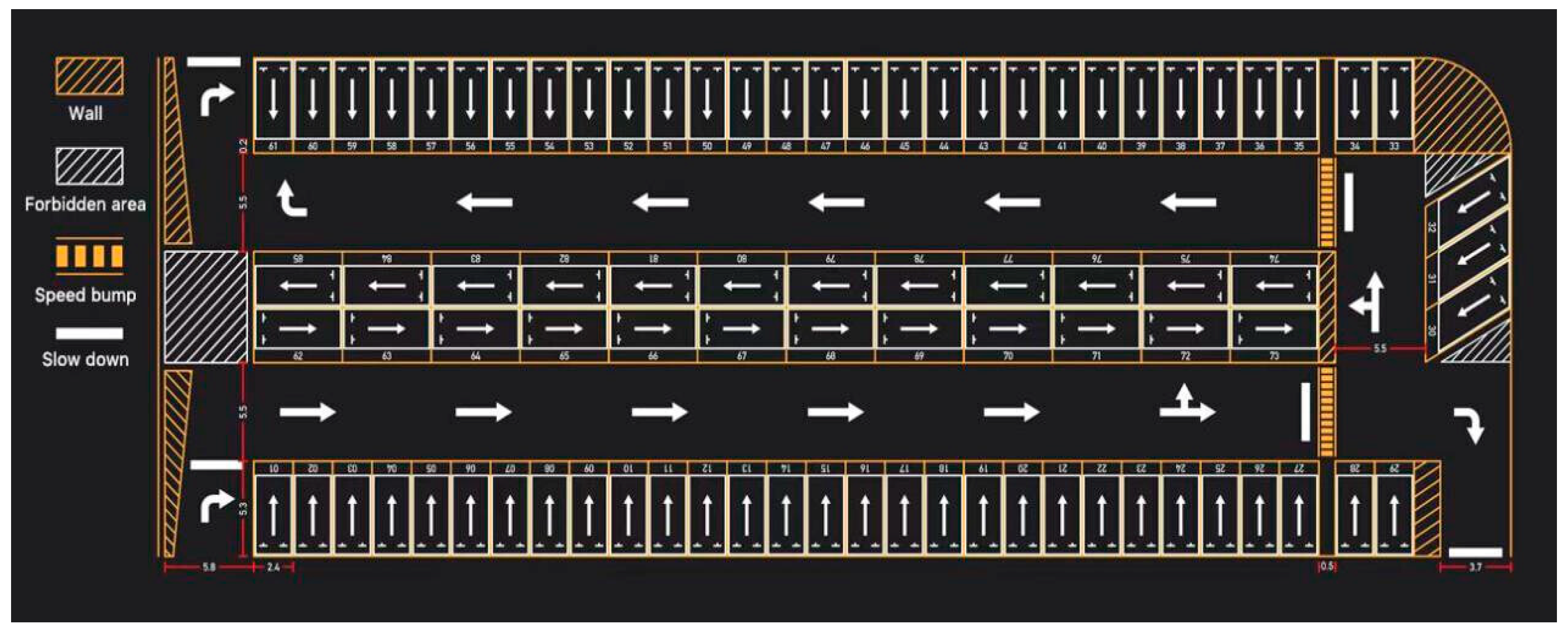
2.2. Parking Lot Plan Model

The indoor parking lot of a shopping mall in Xuanwu District, Nanjing, is selected as the reference model for this study, as shown in Figure 2. There is one entrance and two exits in the parking lot. The parking spaces are numbered from 1 to 85 and arranged counterclockwise from the periphery to the inner periphery. The lane width is 5.5 m. The types of parking spaces include parallel, perpendicular, and angled parking spaces. The orange diagonal lines are the parking walls, and the white diagonal lines are the no-parking areas with other uses.

2.3. Entropy Method [16,17,18,19]

The entropy weight method is an objective weighting method, the basic idea of which is to determine the objective weights according to the magnitude of the variability of the indicators. Based on the principle that the smaller the variability of an indicator, the less information it reflects, the lower the corresponding weight should be.

(1) Preprocessing of data: Assume that there are n objects to be evaluated, and m evaluation indicators (which have been normalized) constitute the normalization matrix as follows.

$$X=\left[\begin{array}{llll}{x}_{11}& x_{12}& \cdots & x_{1m}\\ x_{21}& x_{22}& \cdots & x_{2m}\\ ⋮& ⋮& \ddots & ⋮\\ x_{n1}& x_{n2}& \cdots & x_{nm}\end{array}\right]$$

(11)

The data are normalized, and the normalized matrix is denoted as Z. For each element in Z,

$$z_{ij}=x_{ij}/\sqrt{{\displaystyle \sum _{i=1}^n{x}_{ij}^2}}$$

(12)

This equation is used to determine whether there are negative numbers in the Z matrix, if so, another normalization method is needed for X. The matrix X is normalized once by the following formula.

$$\widetilde{Z_{ij}}=\frac{x_{ij}-\min \left\{x_{1j},x_{2j},\dots ,x_{nj}\right\}}{\max \left\{x_{1j},x_{2j},\dots ,x_{nj}\right\}-\min \left\{x_{1j},x_{2j},\dots ,x_{nj}\right\}}$$

(13)

(2) Calculate the weight of the ith sample under the jth indicator and consider it as the probability used in the relative entropy calculation; then, calculate the probability matrix P on the basis of the previous step, with each element in P as follows.

$$p_{ij}=\frac{\widetilde{z_{ij}}}{{\displaystyle \sum _{i=1}^n{z}_{ij}}}$$

(14)

(3) Calculate the information entropy of each indicator, calculate the information utility value, and normalize it to obtain the entropy weight of each indicator for the jth indicator, whose information entropy is calculated by the following formula.

$$e_{ij}=-\frac{1}{\ln n}{\displaystyle \sum _{i=1}^n{p}_{ij}\ln \left(p_{ij}\right)}\left(j=1,2,\dots ,m\right)$$

(15)

The larger e_j is, the greater the information entropy of the jth indicator, and the smaller its corresponding information quantity. Defining the information utility value dj, the formula is as follows.

$$d_j=1-e_j$$

(16)

Normalize the information utility values to obtain the entropy weight of each indicator.

$$W_j=d_j/{\displaystyle \sum _{j=1}^m{d}_j}$$

(17)

2.4. Bayesian Networks [20,21,22,23]

Bayesian networks can be learned automatically directly from a database using empirically based algorithms that are usually built into appropriate software. Bayesian networks are well-suited for obtaining events that have occurred and predicting any one of several possible known causes.

Bayesian network model conditional dependence by representing conditional dependence through edges in the structure, and by extension, causation. Through these relationships and the use of factors, we can make effective inferences about random variables. The joint distribution of a Bayesian network is equal to the product of P (node|parent) of all nodes, as follows.

$$\begin{array}{l}P\left(X_1,\dots ,X_n\right)\\ ={\displaystyle \prod _{i=1}^{n}P\left(X_i|X_1,\dots ,X_{i-1}\right)}\\ ={\displaystyle \prod _{i=1}^{n}P\left(X_i|Parents\left(X_i\right)\right)}\end{array}$$

(18)

Inference in Bayesian networks takes two forms. The first approach is to simply evaluate the joint probability of a particular assignment of each variable (or subset) in the network. The second approach is to find P(x|e), or the probability of an assignment of a subset of variables given other variable assignments (x), where we must marginalize the joint probability distribution of variables that do not appear in x or e, which we denote as Y.

$$P\left(x|e\right)=\alpha {\displaystyle \sum _{\forall y\in Y}P\left(x,e,Y\right)}$$

(19)

2.5. Principle of KMO Test [24]

KMO is the abbreviation of Kaiser–Meyer–Olkin, which is an index to measure the close relationship between variables in factor analysis.

Suppose two samples are randomly selected from the overall sample pool $\left(X_i,Y_i\right)\left(i=1,2,3\cdots n\right)$; then, the coefficient of the simple linear relationship between the two samples is obtained as follows.

$$p=\frac{{\displaystyle \sum _{i=1}^n\left(X_i-\overline{X}\right)}\left(Y_i-\overline{Y}\right)}{\sqrt{{\displaystyle \sum _{i=1}^n{\left(X_i-\overline{X}\right)}^2}}\sqrt{{\displaystyle \sum _{i=1}^n{\left(Y_i-\overline{Y}\right)}^2}}}$$

(20)

$$\overline{X}=\frac{1}{n}{\displaystyle \sum _{i=1}^n{X}_i}$$

(21)

$$\overline{Y}=\frac{1}{n}{\displaystyle \sum _{i=1}^n{Y}_i}$$

(22)

The bias correlation coefficient is more able to reflect the intrinsic relationship between different variables by excluding the interference of other factors when the rest of the variables are determined. Equation (23) is the formula for the second-order bias correlation coefficient, and Equation (24) is the formula for the multi-order bias correlation coefficient.

$$r_{xy,z_1}=\frac{r_{xy}-r_{x{z}_1}{r}_{y{z}_1}}{\sqrt{\left(1-r_{x{z}_1}{}^2\right)\left(1-r_{y{z}_1}{}^2\right)}}$$

(23)

$$r_{xy,z_1,z_2\cdots z_h}=\frac{r_{xy,z_1,z_2\cdots z_{h-1}}-r_{x{z}_h{}_{,z_1},z_2\cdots z_{h-1}}}{\sqrt{\left(1-r_{xy,z_1,z_2\cdots z_{h-1}}{}^2\right)\left(1-r_{y{z}_h{}_{,z_1},z_2\cdots z_{h-1}}{}^2\right)}}$$

(24)

where $r_{xy}$ is a simple correlation between $X$ and $Y$, and $z_1,z_2\cdots z_h$ is the identified $h$ variable.

The KMO value of the sample data is expressed as the weight of the sum of the simple correlation coefficients of the sample variables in relation to the sum of the simple and partial correlation coefficients.

$$PP={\displaystyle \sum {{\displaystyle \sum _{i\ne j}{r}_{ij}}}^2}$$

(25)

$$RR={\displaystyle \sum {{\displaystyle \sum _{i\ne j}{r}_{ij,z_1,z_2\cdots z_k}}}^2}$$

(26)

$$KMO=\frac{PP}{PP+RR}$$

(27)

In 1974, Kaiser [25] published an article named ‘An index of factorial simplicity’ in the journal Psychometrika, which stipulated that the value of KMO was 0–1. For $KMO$ $\left[0,1\right]$, the closer the value to 1, the stronger the correlation between the variables, and the more suitable all the variables are for factor analysis; the closer the value to 0, the weaker the correlation between the variables, and the less suitable all the variables are for factor analysis.

Table 1. Table of KMO test criteria.

Test Category	Range of Values	Factor Analysis is Appropriate for the Situation
$KMO$	$\left(0.9,1\right]$	Perfect for
	$\left(0.8,0.9\right]$	Great for
	$\left(0.7,0.8\right]$	Suitable for
	$\left(0.6,0.7\right]$	Barely fit
	$\left(0.5,0.6\right]$	Not really suitable
	$\left[0,0.5\right]$	Not suitable

shows the suitability of $KMO$ for factor analysis at different values.

3. Analysis and Results Discussion

3.1. Vehicle Parking Path Planning

For a visual demonstration, we chose parking spaces 10, 31, and 82 as examples, as shown in Figure 3.

3.1.1. Vertical Parking

Vertical Parking Path Planning

For the vehicle from the parking space entrance along a straight line, then through the arc trajectory into the horizontal section, and then forward a distance after the vehicle’s control point to the right edge of the parking space with 11 in the same horizontal position. It began to reverse along the arc into the parking space and then along the straight line, it went forward a distance to the target parking position of such a reverse process using reverse thinking as shown in Figure 4, in order to facilitate the solution of the vehicle parking trajectory problem, simplify the complexity of the model, and give priority to the car in a straight line and arc on the reverse motion process; remember that the arc endpoints do not meet the endpoint of a straight line for the initial position.

When the initial position of the vehicle meets the requirement of one-step perpendicular parking, the parking-assisted parking system issues a command, and the vehicle owner can preferentially choose to reverse into the parking space according to the one-step perpendicular parking trajectory.

The geometric relationship between the turning radius of the vehicle $R_1$ and the horizontal coordinates of the initial position of the vehicle and the width of the parking space is reacted in Equations (28) and (29).

$$s_2=s-s_1$$

(28)

$$s_2=R_1$$

(29)

where $s$ is the horizontal coordinate value of the initial position where the vehicle starts reversing into the $1/4$ arc.

The relationship with the width of the parking space $W_p$ is shown in Equation (30).

$$s_1=W_p/2$$

(30)

The relationship between the turning radius and the value of the horizontal coordinate of the initial position of the vehicle starting to reverse into the arc of $1/4$ and the width of the parking space $W_p$ can be obtained by combining Equations (28)–(30), as shown in Equation (31).

$$R_1=s-W_p/2$$

(31)

When the starting position of the vehicle does not meet the requirement of one-step vertical parking, a three-step vertical parking path planning is required, as shown in Figure 5.

For the three-step vertical parking path planning, given the limitation of parking space size and shape, the minimum turning radius is utilized as the radius of the circular arc trajectory when the vehicle reverses into the parking space, as shown in Figure 5. The vehicle quickly turns the steering wheel to the maximum turning angle from the starting position $C$ at the maximum steering wheel speed to drive in reverse. When the control point of the vehicle, i.e., the center point of the rear axle, reaches the center axis of the 10th parking space, the vehicle no longer runs in reverse, but turns the steering wheel rapidly to the maximum turning angle at the maximum speed in the direction opposite to that of the backward direction for forward driving until the point $E$, and again turns the steering wheel rapidly to the maximum turning angle at the maximum speed to drive in reverse until the control point of the vehicle reaches the tangent to the center point of the rear axle. When the vehicle control point of the vehicle reaches the point $F$, which is tangent to the center point, turn the steering wheel to return to the original position, and the vehicle then moves in a straight line in the vertical direction along the center axis of the parking space $10$ until it reaches the target parking point.

There is a numerical relationship between the three steering angles in Figure 5, as shown in Equation (32).

$${\theta }_1+{\theta }_2+{\theta }_3=\pi /2$$

(32)

Analysis of Vertical Parking Obstacle Avoidance

For the vehicle parking process, multiple boundary conditions need to be considered as shown in Figure 6, such as the car cannot touch the boundary of the parking space, the road boundary, etc. In addition to meeting the basic conditions of not wanting to touch, the safety of the vehicle is fully considered, and the safety distance needs to be set for different boundaries. When the car is driven in the area delineated by these safety distance lines, the safety of the vehicle driving is improved, while the possibility of collision with the boundary is further reduced.

Therefore, the following constraints need to be considered in the process of parking a vehicle into a parking area.

(1)

The vehicle apex $e$ does not collide with the left parking space boundary.

$$\{\begin{array}{l}{x}_{O_1}=O_1{e}^{\prime }\\ O_1{e}^{\prime }=O_{1}e\\ O_{1}e=\sqrt{{\left(R_1+w/2\right)}^2+l_r{}^2}\\ x_{O_1}\ge O_{1}e\end{array}$$

(33)

(2)

The vehicles do not collide with obstacles on the right.

$$\{\begin{array}{l}{O}_1{P}_1=O_1{m}^{\prime }\\ O_1{m}^{\prime }=O_{1}m\\ O_{1}m=R_1-w/2\\ O_1{P}_1=\sqrt{{\left(x_{O_1}-W_p\right)}^2+\left(y_C-R_1\right)}\\ O_1{P}_1\le R_1-w/2\end{array}$$

(34)

(3)

The vehicles sit on top of the apex and road boundaries without colliding.

$$\{\begin{array}{l}{O}_1{f}^{\prime }=O_{1}f\\ O_{1}f=\sqrt{{\left(R_1+w/2\right)}^2+{\left(l+l_r\right)}^2}\\ O_{1}f-R_1+y_C\le L_{road}\end{array}$$

(35)

In order to reduce the possibility of the vehicle in the parking process and parking space edge or road edge and other obstacles’ edge collision, in the analysis of the vehicle driving trajectory, the obstacles to add a safety distance $d_3$ are considered, and from the analysis of the minimum turning radius, parking space width, and other geometric factors, there is a certain value relationship, as shown in Equation (36).

$$\begin{array}{c}\sqrt{{\left(x_{O_1}-W_p\right)}^2+{\left(R_{\min }-w/2-d_3\right)}^2-{\left(R_{\min }-W_p/2\right)}^2}+d_3\\ =R_{\min }-w/2\end{array}$$

(36)

$$x_{O_1}=R_{\min }+W_p/2$$

(37)

By calculating Equation (42), we can obtain the lower limit extreme value of the vertical coordinate $y_c$ at the point $C$

$$y_C=R_{\min }-\sqrt{{\left(R_{\min }-w/2-{\mathrm{d}}_3\right)}^2-{\left(R_{\min }-W_P/2\right)}^2}$$

(38)

The horizontal and vertical coordinates of point D are as follows.

$$\begin{array}{l}{x}_D=W_p/2\\ y_D=-\sqrt{{\left(R_{\min }-w/2-d_3\right)}^2-{\left(R_{\min }-W_p/2\right)}^2}\end{array}$$

(39)

$$\begin{array}{l}{x}_{C_{\max }}=R_1+W_p/2\\ y_{C_{\max }}=R_1+y_D\end{array}$$

(40)

$$\sqrt{{\left(R_1+w/2\right)}^2+{\left(l+l_r\right)}^2}-R_1+y_C\le L_{road}$$

(41)

$$y_C=R_1+y_D$$

(42)

$$x_{O_1}=\sqrt{{\left(R_1+w/2\right)}^2+l_r{}^2}$$

(43)

According to the spatial situation of the parking lot, the starting area where the vehicle may temporarily stay before parking is delineated using the parking space to be parked as the reference system, and four different boundary lines are determined based on the above boundary conditions for calculation, as shown in Figure 7. The expression of boundary line 1 is ${\left(x-2.4\right)}^2+{\left(y-4.98\right)}^2={4.08}^2$, the expression of boundary line 2 is $x=5.973$, the expression of boundary line 3 is $y=3.452$, and the expression of boundary line 4 is y = 3.01. When the vehicle is initially in the area below boundary line 4, the parking operation cannot be completed by one-step parking due to the limitation of parking space size, and the parking can only be completed by three-step parking. The vehicle can be parked in one step only when the vehicle control point position is located in the sector-like area enveloped by boundary line 1, boundary line 2, boundary line 3, and boundary line 4.

Vertical Parking Trajectory

In order to ensure safety and to make the time as small as possible, we choose one-step parking, i.e., the starting point of parking is located in the area below line 3 and above line 4.

The point in Figure 4 (5.6 m, 3.45 m) is selected as the starting point and modeled as follows.

t₁ is the time to do accelerated motion with changing acceleration, the velocity is v1, and the acceleration is a₁.

A uniform 1/4 circular motion in the time period t₂ is selected.

An accelerated motion with increasing acceleration in the time period t₃ is selected.

Uniform motion during the time period t₄ is selected.

t₅ is the time period for decelerating motion.

$$\{\begin{array}{l}\min t=t_1+t_2+t_3+t_4+t_5\\ t_1=v_1/a_1\\ 0\le a_1\le 3\\ -5\le d_2\le 0\\ t_2=\frac{1}{2}\cdot \frac{\pi R_k}{v_1}\\ \frac{d{a}_1}{dt}\le 20\\ v_2=v_1+a_1{t}_3\\ v_3=v_2+a_2{t}_4\\ v_3=0\\ v_1{t}_3+\frac{1}{2}{a}_1{t}_3{}^2+v_2{t}_4+\frac{a_2}{2}{t}_4{}^2=2.4\times 9+s\\ t_{{}_5}=\frac{\theta R_k}{v_1}\end{array}$$

(44)

By solving the above model, it can be seen that the vertical parking trajectory is shown in Figure 8.

The variation of speed, acceleration, and path of the vehicle from the beginning of the movement with time are shown in

Table 2. Vehicle trajectory—time variation.

$\mathit{t}$/s	$\mathit{v}$/m/s	$\mathit{x}$/m	$\mathit{a}$/m/s2	${\mathit{a}}^{\prime }$/m/s3	$\mathit{\theta }/°$
0	0	0	0	0	90
0.15	0.25	0.01125	3	20	90
0.59	1.544	0.4	3	0	90
7.082	1.544	10.423	0	0	0
7.232	1.769	10.655	3	20	0
8.494	5.556	20.055	3	0	0
10.619	5.556	31.863	0	0	0
10.919	4.656	33.348	−6	−20	0
11.695	0	35.155	−6	0	0

.

3.1.2. Parallel Parking

Parallel Parking Path Planning and Obstacle Avoidance Analysis

In order to make the parking path and time as short as possible, the turning radius of the last segment of the circular path of parking is set as the minimum turning radius, and the position of the starting point of the straight segment of the path is as close as possible to the origin of the coordinate system. First, the minimum parking space size for parallel parking is determined. As shown in Figure 9, the size of the minimum parking space required for parallel parking is mainly related to the second segment of the circular arc path, and the radius of the second segment of the circular arc path is the minimum turning radius to avoid collision as much as possible. Using the inverse planning method, it is assumed that the vehicle is parked at the target location of the parking space, and the vehicle can drive out of the parking space safely and smoothly according to the planned path FE and finally finish parking along the path. The vehicle does not collide with the P₁ point of the right obstacle in the process of driving out, then the minimum parking space length is calculated at this time as the minimum parking space length. Then, the vehicle b points to O₁ as the center of the circle, and R_b is the radius of driving to the b′ point. The b′ point and P₁ point distance should not be less than the safety distance d₁. According to the geometric relationship, we can derive the minimum parking space length $L_{\min }$ as follows.

$$L_{\min }=d_2+l_r+\sqrt{R_b{}^2-{\left(R_{\min }-w/2\right)}^2}+d_1$$

(45)

$$R_b=\sqrt{{\left(R_{\min }+w/2\right)}^2+{\left(l+lr\right)}^2}$$

(46)

When the safety distance d₁ tends to 0, the minimum parking space length L_min = 6.772 m, which is larger than the actual parking space length. Therefore, cars in the parking lot cannot be parked in one step but can only be parked in multi-step mode.

Parallel Parking Trajectory

According to the vehicle parking conditions and obstacle avoidance requirements, the following parallel parking model is established.

$$\{\begin{array}{l}\min T=t_1+t_2+t_3+t_4+t_5+t_6+t_7\\ 0\le a_1\le 3\\ -5\le a_2\le 0\\ \frac{v_1{}^2}{2a_1}=0.4\\ t_2=\frac{1}{2}\cdot \frac{\pi R_k}{v_1}\\ 0\le \frac{d{a}_1}{dt}\le 20\\ -20\le \frac{d{a}_2}{dt}\le 0\\ 0\le \frac{d{a}_3}{dt}\le 20\\ -20\le \frac{d{a}_4}{dt}\le 0\\ v_2=v_1+a_1{t}_3\\ v_3=2.77\left(10km/h\right)\\ t_4=\frac{v_2-v_3}{a_2}\\ v_1{t}_3+\frac{1}{2}{a}_1{t}_3{}^2+v_2{t}_4+\frac{1}{2}{a}_2{t}_4{}^2=27\times 2.4-5\end{array}$$

(47)

The model is solved to ensure safety and the smallest possible time, and the parallel parking trajectory is shown in Figure 10.

3.1.3. Inclined Parking

Inclined Parking Path Planning

As shown in Figure 11, the diagonal parking path consists of two parts: First, the target vehicle starts backing up in reverse at the starting point C, with the point O’ as the center of the circle and the turning radius R. When the vehicle heading angle is $\beta -\frac{\pi }{2}$ turn the steering wheel and start to back up along a straight line to the parking point E to complete the parking.

The turning radius is as follows.

$$R=\frac{s-s_1}{\sin \alpha }$$

(48)

where $\alpha$ is the turning angle during the vehicle movement, $\alpha =\pi -\beta$.

Obstacle Avoidance Analysis of Inclined Parking Path

When the target vehicle is being parked, two types of collisions may occur for parking situations where its final parking space axis position has been determined: the intersection position of the vehicle’s rear axis extension line and the body may collide with the right obstacle, and the left front vertex of the vehicle may collide with the road boundary. The constraint conditions are as follows.

$$R_{\min }-w/2\ge \sqrt{{\left(x_c-x_{P_1}\right)}^2+{\left(R_{\min }-y_c\right)}^2}$$

(49)

$$L_{road}+R_1-y_c\ge \sqrt{{\left(R_1+w/2\right)}^2+{\left(l+l_f\right)}^2}$$

(50)

Since the previous two parking methods were analyzed in detail and the analysis process of inclined parking is the same as shown in Figure 12, no specific analysis will be done here.

3.2. Optimal Berth Selection

3.2.1. Static Optimal Parking Space Selection Based on Entropy Weight Method

Parking Space Attributes

The entire parking lot has 85 parking spaces as shown in Figure 13. Considering that spaces 1, 3, 4, 6–8, 10–12, 14–44, 45, 48, 50, 51, 55–63, 65, 66, 68–77, 79, 80, and 83–85, a total of 70 parking spaces, are red prohibited parking, meaning that they have been occupied, that leaves spaces 2, 5, 6, 13, 45, 47, 49, 52, 53, 54 64, 67, 78, 81, and 82, so a total of 15 free parking spaces are available.

Types of Parking Spaces

It is known that the vacant parking spaces are divided into three kinds of vertical parking spaces, parallel parking spaces, and inclined parking spaces. The difficulty of parking in these three kinds of spaces varies, from the perspective of practical experience, the difficulty of parking in vertical parking spaces, the difficulty of parking in parallel parking spaces, and the difficulty coefficient of parking in inclined parking spaces are all between $\left[0 , 1\right]$, taking the following.

$$p_1=\left[\begin{array}{l}\mathrm{vertical} \mathrm{parking} \mathrm{difficulty},\\ \mathrm{parallel} \mathrm{parking} \mathrm{difficulty}, \\ \mathrm{inclined} \mathrm{parking} \mathrm{difficulty}\end{array}\right]$$

(51)

$$p_1=\left[1,0.5,0.8\right]$$

(52)

At this point, the parking difficulty of the available parking spaces 2, 5, 6, 13, 45, 47, 49, 52, 53, 54, 64, 67, 78, 81, and 82 can be expressed according to their parking space type by the vector $p_2$ as follows.

$$p_2=\left[0.5,0.5,0.5,0.5,0.5,0.5,0.5,0.5,0.5,0.5,1,1,1,1,1\right]$$

(53)

Left and Right Situation

From actual experience, it is known that the parking space left and right space occupancy also affects the parking difficulty. Generally speaking, the less the number of occupied parking spaces, the easier it is to park and the lower the parking difficulty factor; the more the target parking space is occupied, the more difficult it is to park and the higher the parking difficulty factor. The parking space is divided into four cases: left and right parking spaces are occupied, left parking spaces are occupied, right parking spaces are occupied, and left and right parking spaces are vacant. From the perspective of practical experience, the parking difficulty coefficients of these four situations are between $\left[0,1\right]$, and the orientation quantity $p_1$ indicates the parking difficulty coefficient of the above four situations for the left and right parking occupancy, as shown in the Equations (54) and (55):

$$p_3=\left[\begin{array}{l}\mathrm{left} \mathrm{and} \mathrm{right} \mathrm{parking} \mathrm{spaces} \mathrm{occupied},\\ \mathrm{left} \mathrm{parking} \mathrm{spaces} \mathrm{occupied}, \\ \mathrm{right} \mathrm{parking} \mathrm{spaces} \mathrm{occupied},\\ \mathrm{left} \mathrm{and} \mathrm{right} \mathrm{parking} \mathrm{spaces} \mathrm{vacant}\end{array}\right]$$

(54)

$$p_3=\left[1,0.6,0.7,0.5\right]$$

(55)

At this point, the parking difficulty of the available parking spaces 2, 5, 6, 13, 45, 47, 49, 52, 53, 54, 64, 67, 78, 81, and 82 can be expressed by the vector $p_4$ according to the occupancy of their left and right parking spaces as follows.

$$p_4=\left[1,1,1,1,1,1,1,0.6,0.5,0.7,1,1,1,0.6,0.7\right]$$

(56)

3.2.2. Distance

In addition to considering the difficulty of parking with different types of parking and different occupied left and right parking spaces, the selection of the optimal parking space also needs to consider the distance from the starting point to the target parking space of the car and the walking distance that the occupant or driver needs to walk to leave the parking lot after parking is completed, so the distance from the starting point to different free parking spaces of the car needs to be included in the analysis.

In order to more conveniently represent the distance from the starting point of vehicle parking to the target parking space, a Cartesian coordinate system is established to conveniently represent the coordinate positions of different parking spaces and the distance from the starting point to the target parking space by combining the starting position with the location distribution of available free parking spaces. The coordinates of parking spaces are calculated by the center point of the parking spaces.

For this, the coordinates of the vehicle control point are set as the coordinate origin, the horizontal direction as the horizontal axis, the horizontal direction to the right as the horizontal axis positive, the vertical direction as the vertical axis, and the vertical direction up as the vertical axis positive.

The locations of the 15 available free parking spaces are represented by coordinates as shown in

Table 3. Coordinates of vacant parking spaces.

Vacant Parking Space Number	Coordinate Location
2	(−57.35, −5.7)
5	(−50.15, −5.7)
6	(−40.55, −5.7)
13	(−30.95, −5.7)
45	(−21.35, 16.2)
47	(−26.15, 16.2)
49	(−30.95, 16.2)
52	(−38.15, 16.2)
53	(−40.55, 16.2)
54	(−42.95, 16.2)
64	(−44.6, 4.15)
67	(−29.3, 4.15)
78	(−19.1, 6.55)
81	(−34.4, 6.55)
82	(−39.5, 6.55)

.

Based on the coordinate locations of the free parking spaces in Table 3 and the direction of road access in the parking lot of this question, the distance between the location of these 15 available free spaces and the location of the starting point for the vehicle parking can be calculated as shown in the vector $p_3$, and the results are summarized in

Table 4. Parking attribute normalization matrix.

Parking Space Number	p1 (Type of Parking Space)	p2 (Left and Right Cases)	p3 (Distance)
2	0	1	1.00
5	0	1	0.81
9	0	1	0.55
13	0	1	0.30
45	0	1	0.18
47	0	1	0.28
49	0	1	0.39
52	0	0.2	0.57
53	0	0	0.63
54	0	0.4	0.69
64	1	1	0.66
67	1	1	0.25
78	1	0.2	0.00
81	1	0.4	0.40
82	1	1	0.53

and

Table 5. Entropy matrix of parking attributes.

Parking Space Number	p1 (Type of Parking Space)	p2 (Left and Right Cases)	p3 (Distance)
2	0.05	0.08	0.10
5	0.05	0.08	0.09
9	0.05	0.08	0.07
13	0.05	0.08	0.05
45	0.05	0.08	0.05
47	0.05	0.08	0.05
49	0.05	0.08	0.06
52	0.05	0.05	0.07
53	0.05	0.04	0.08
54	0.05	0.05	0.08
64	0.1	0.08	0.08
67	0.1	0.08	0.05
78	0.1	0.05	0.04
81	0.1	0.05	0.06
82	0.1	0.08	0.07

.

$$p_3=\left[\begin{array}{l}57.63,50.47,40.95,31.47,26.80,\\ 30.76,34.93,41.45,43.67,45.90,\\ 44.79,29.59,20.19,35.02,40.04\end{array}\right]$$

(57)

Combining the above-mentioned different types of parking methods and the difficulty of parking under the left and right occupancy of different parking spaces, the attribute information of parking in different vacant parking spaces is represented as matrix R₀:

$$R_0={\left[\begin{array}{rrr}\hfill 0.5& \hfill 1& \hfill 57.63\\ \hfill 0.5& \hfill 1& \hfill 50.47\\ \hfill 0.5& \hfill 1& \hfill 40.95\\ \hfill 0.5& \hfill 1& \hfill 31.47\\ \hfill 0.5& \hfill 1& \hfill 26.80\\ \hfill 0.5& \hfill 1& \hfill 30.76\\ \hfill 0.5& \hfill 1& \hfill 34.93\\ \hfill 0.5& \hfill 0.6& \hfill 41.45\\ \hfill 0.5& \hfill 0.5& \hfill 43.67\\ \hfill 0.5& \hfill 0.7& \hfill 45.90\\ \hfill 1& \hfill 1& \hfill 44.79\\ \hfill 1& \hfill 1& \hfill 29.59\\ \hfill 1& \hfill 0.6& \hfill 20.19\\ \hfill 1& \hfill 0.7& \hfill 35.02\\ \hfill 1& \hfill 1& \hfill 40.04\end{array}\right]}^T$$

(58)

Each column of matrix R₀ represents the attribute information of a parking space, including the type of parking space (vertical parking space, parallel parking space, inclined parking space), the left and right occupancy of the parking space (both left and right parking spaces are occupied, left parking space is occupied, right parking space is occupied, or both left and right parking spaces are free), and the distance between the location of the free parking space and the location of the starting point where the vehicle temporarily stays. Each row of the matrix R₀ represents one free parking space.

Based on the current parking space usage, the optimal parking space is selected from the remaining available free parking spaces. An evaluation matrix of the parking difficulty and driving walking distance of different parking spaces can be established, and the selection of the optimal parking space is determined by the evaluation scores of the different parking spaces. After the analysis, the comprehensive difficulty coefficient matrix of different available parking spaces $R_0$ is derived, and in order for it to be applied to the next factor analysis, it is first necessary to perform the $KMO$ test.

After calculating the values of $KMO$ for the evaluation matrix $R_0$, we get

$$KMO\left(R_0\right)=0.4642$$

(59)

According to the test table of $KMO$, it can be obtained that the correlation value between the variables of $KMO$ is weak at less than 0.5, which is not suitable for factor analysis, so it is considered that there is no correlation between the attributes of each available vacant parking space, and there is no need to perform factor rotation and factor score calculation for $R_0$; instead, $R_0$ can be used directly as the original evaluation matrix of entropy weight method.

Table 6. Parking attribute weighting.

Properties	p1 (Type of Parking Space)	p2 (Left and Right Cases)	p3 (Distance)
Weights	0.517	0.211	0.272

shows the weights of the three attributes of parking space type, parking space left and right situation, and distance between starting point and parking space in the optimal parking space selection process calculated by the entropy weight method.

The weight results of each attribute in Table 6 show that the weight of the parking space type is the largest, and the weight of the parking space left and right situation is the smallest, indicating that the parking space type has the greatest degree of influence on the final choice in the process of making the best parking space selection. Combined with the real situation, the type of parking space in the actual scenario largely affects the driving trajectory of the parking process and puts more space restrictions on the actual safe area where the vehicle can be parked compared to the parking space occupied by the left and right parking spaces. The walking distance of passengers and drivers is not very large because the parking lot is not very large, taking into account the limitation of its size and making the weight of the consideration of the walking distance not as heavy as the type of parking space in practice. Therefore, it is considered that the values of the weight of each attribute of the parking space obtained from Table 6 have a strong practical significance.

Table 7. Parking difficulty score by parking space.

Parking Space Number	Difficulty Score
2	0.23
5	0.21
9	0.18
13	0.15
45	0.14
47	0.15
49	0.16
52	0.09
53	0.07
54	0.13
64	0.96
67	0.91
78	0.79
81	0.86
82	0.95

shows the difficulty scores of each parking space after combining three factors: type of parking space, left and right use of parking space, and walking distance. The higher the difficulty score, the more difficult it is to park in this space, and the less likely it is to successfully park in this space and meet the walking distance requirement; conversely, the lower the difficulty score, the more difficult it is to park in this space.

From Table 7, it can be seen that parking space 53 has the lowest overall parking difficulty score and the lowest difficulty factor and is the best parking space among the 15 free available spaces in this question.

When the user enters the parking lot, the parking-assisted parking system will inform the car owner that parking space 53 is the best parking space. Considering the actual situation that parking space 53 is a vertical parking space, the left and right parking spaces are not occupied and are free and available, there is a certain distance between the parking space position and the starting position—but it is not the farthest among the 15 free and available parking spaces, and the walking distance factor has the least weight among the three attributes, it is considered that parking space 53 is the best parking space.

3.2.3. Dynamic Optimal Parking Space Selection Based on Entropy Weight Method and Bayesian Network

As there are vehicles entering and leaving the parking lot every hour, the current parking space will be occupied or vacant at random. Although it is not possible to artificially determine the specific number of vehicles present in the parking lot and the parking space situation at the next moment, with the help of Bayesian networks, it is possible to account for and learn the probability of the available parking spaces and the number of parking spaces in the parking lot at the previous moment based on the computer clock (the optimal parking space is parking space 53 when there were only 15 free parking spaces among parking spaces 1–85 at the previous moment). This is used to infer the situation in the parking lot at the next moment. After the careful inference of Bayesian network, the new parking situation in the parking lot is obtained as shown in Figure 14, and then combined with the entropy weight method, so as to establish the dynamic optimal parking space selection model.

When the parking lot space usage changes dynamically, different space occupancy will affect the motion trajectory into the optimal parking space obtained from the above stationary state to some extent and change the parking difficulty while affecting the vehicle trajectory, so the already derived parking difficulty score table for each parking space needs to be updated.

First, the attribute information matrix $R_0$ for empty parking spaces is updated.

$$R_1={\left[\begin{array}{lll}0.5\hfill & 1\hfill & 17.06\hfill \\ 0.5\hfill & 1\hfill & 14.10\hfill \\ 0.5\hfill & 1\hfill & 17.06\hfill \\ 0.5\hfill & 1\hfill & 34.24\hfill \\ 0.5\hfill & 1\hfill & 34.03\hfill \\ 0.5\hfill & 1\hfill & 19.94\hfill \\ 0.5\hfill & 1\hfill & 15.38\hfill \\ 0.5\hfill & 1\hfill & 11.01\hfill \\ 0.5\hfill & 0.7\hfill & 5.91\hfill \\ 0.5\hfill & 0.6\hfill & 5.40\hfill \\ 0.5\hfill & 1\hfill & 11.13\hfill \\ 1\hfill & 1\hfill & 9.09\hfill \\ 1\hfill & 1\hfill & 17.01\hfill \\ 1\hfill & 0.6\hfill & 7.54\hfill \\ 1\hfill & 0.5\hfill & 4.32\hfill \\ 1\hfill & 0.6\hfill & 5.69\hfill \end{array}\right]}^T$$

(60)

The updated $R_0$ will have the same meaning as the original $R_0$.

The updated matrix $R_1$ was first subjected to factor analysis, which after the KMO test yielded the following.

$$KMO\left(R_1\right)=0.5271$$

(61)

After observing the calculated values of KMO of the matrix $R_1$, we can find that the correlation of the matrix $R_1$ is very poor. It can be seen that the three factors selected here are independent of each other and have some reasonableness, so there is no need to do factor analysis, and $R_1$ can be used directly as the original evaluation matrix of the entropy weight method.

The weights of the three attributes of parking space type, parking space occupancy to the left and right of the parking space, and the distance between the target parking space and the starting position are reassigned by the entropy weight method, and the obtained results are shown in Figure 15.

After the update, the weight of the type of parking space is 0.22, the weight of the left and right occupancy of the parking space is 0.1, and the weight of the distance is 0.68.

The attribute with the highest weight value is distance. The distance of the vehicle from different parking spaces is plotted as shown in Figure 16, and this distance plays a dominant role in the score of the difficulty of parking all the vehicles.

From Figure 17, the parking difficulty score shows that parking space 81 has the smallest comprehensive parking difficulty score and the lowest difficulty coefficient. Under the situation that vehicles enter and leave the parking lot every hour and each parking space will be occupied or released randomly, parking space 81 is the optimal parking space under the dynamic change of parking space occupation. The parking assistance system will indicate to the car owner that parking space 81 is the best parking space.

From the actual situation, parking space 81 is a parallel parking space, the left side of parking space 82 is not occupied—so it is in the free available state, the travel distance between parking space 81 and parking space 51 is close, and there are adjacent free parking spaces around, so parking space 81 is considered to be the best parking space in line with the actual situation and subjective understanding.

4. Conclusions

In summary, the proposed parking assistance method based on the entropy power method and Bayesian network for optimal parking and parking path planning is used for parking path optimization and selecting parking spaces. The main conclusions are summarized below:

(1)

Clear and specific analysis of the obstacles when parking the vehicle into the parking space is demonstrated with good consistency, and the parking guidance trajectory given by the parking assistance parking system is both safe and fast.

(2)

In the static case of selecting the optimal parking position, compared with other methods, the proposed method is more lightweight, faster, and more accurate in calculation, and can quickly give feedback on the optimal solution.

(3)

In the dynamic case, the proposed method can learn the situation of the previous moment to reason out the parking space usage condition of the next moment, which is highly sensitive and can adapt well to the change of site conditions, and the auxiliary system could give the car driver a quick guide to find a suitable parking space in a crowded and busy parking lot.

(4)

Based on the findings of this research, the efficient parking path and parking lot selection could be applied in the future rearrangement of indoor parking lots, which could be a feasible way to improve the whole process management sustainability.

Future works: The obstacle settings are all stationary, and no motion obstacle is considered. The speed of the parking process is certain, and the default of the whole parking process is a low-speed motion state, but if the vehicle driving speed is increased, the speed of the vehicle automatic obstacle avoidance turnaround needs to be optimized. At present, it is still in the theoretical design stage, and it is necessary to push the theoretical stage to the experimental stage and promote it to the public.

References

1. Lee, B.; Wei, Y.; Guo, I.Y. Automatic parking of self-driving car based on lidar. Int. Arch. Photogramm. Remote Sens. Spat. Inf. Sci. 2017, XLII-2/W7, 241–246. [Google Scholar] [CrossRef]
2. Zhang, J.; Chen, H.; Song, S.; Hu, F. Reinforcement Learning-Based Motion Planning for Automatic Parking System. IEEE Access 2020, 8, 154485–154501. [Google Scholar] [CrossRef]
3. Gan, N.; Zhang, M.; Zhou, B.; Chai, T.; Wu, X.; Bian, Y. Spatio-temporal heuristic method: A trajectory planning for automatic parking considering obstacle behavior. J. Intell. Connect. Veh. 2022, 5, 177–187. [Google Scholar] [CrossRef]
4. Zhang, C.; Zhou, R.; Lei, L.; Yang, X. Research on Automatic Parking System Strategy. World Electr. Veh. J. 2021, 12, 200. [Google Scholar] [CrossRef]
5. Su, B.; Yang, J.; Li, L.; Wang, Y. Secondary parallel automatic parking of endpoint regionalization based on genetic algorithm. Clust. Comput. 2019, 22, 7515–7523. [Google Scholar] [CrossRef]
6. García, J.M.C.; Piorno, J.R.; Mata-García, M.G. Expert system design for vacant parking space location using automatic learning and artificial vision. Multimed. Tools Appl. 2022, 81, 38661–38683. [Google Scholar] [CrossRef] [PubMed]
7. Oetiker, M.B.; Baker, G.P.; Guzzella, L. A Navigation-Field-Based Semi-Autonomous Nonholonomic Vehicle-Parking Assistant. IEEE Trans. Veh. Technol. 2009, 58, 1106–1118. [Google Scholar] [CrossRef]
8. Zeng, C.; Ma, C.; Wang, K.; Cui, Z.; Dawson, K.A.; Indekeu, J.O.; Stanley, H.E.; Tsallis, C. Predicting vacant parking space availability: A DWT-Bi-LSTM model. Phys. A Stat. Mech. Its Appl. 2022, 599, 127498. [Google Scholar] [CrossRef]
9. Peng, X.; Sun, Z.; Chen, M.; Geng, Z. Arbitrary Configuration Stabilization Control for Nonholonomic Vehicle with Input Saturation: A c-Nonholonomic Trajectory Approach. IEEE Trans. Ind. Electron. 2021, 69, 1663–1672. [Google Scholar] [CrossRef]
10. Aye, Y.Y.; Watanabe, K.; Maeyama, S.; Nagai, I. An automatic parking system using an optimized image-based fuzzy controller by genetic algorithms. Artif. Life Robot. 2016, 22, 1–6. [Google Scholar] [CrossRef]
11. Zhang, P.; Yu, Z.; Xiong, L.; Zeng, D. Research on Parking Slot Tracking Algorithm Based on Fusion of Vision and Vehicle Chassis Information. Int. J. Automot. Technol. 2020, 21, 603–614. [Google Scholar] [CrossRef]
12. Chai, R.; Tsourdos, A.; Savvaris, A.; Chai, S.; Xia, Y.; Chen, C. Design and Implementation of Deep Neural Network-Based Control for Automatic Parking Maneuver Process. IEEE Trans. Neural Netw. Learn. Syst. 2020, 33, 1400–1413. [Google Scholar] [CrossRef] [PubMed]
13. Nakrani, N.M.; Joshi, M.M. A human-like decision intelligence for obstacle avoidance in autonomous vehicle parking. Appl. Intell. 2021, 52, 3728–3747. [Google Scholar] [CrossRef]
14. Lee, C.K.; Lin, C.L.; Shiu, B.M. Autonomous Vehicle Parking Using Hybrid Artificial Intelligent Approach. J. Intell. Robot. Syst. 2009, 56, 319–343. [Google Scholar] [CrossRef]
15. Xie, J.; He, Z.; Zhu, Y. A DRL based cooperative approach for parking space allocation in an automated valet parking system. Appl. Intell. 2022, 53, 5368–5387. [Google Scholar] [CrossRef]
16. Zhang, H.; Jiang, W.; Deng, X. Data-driven multi-attribute decision-making by combining probability distributions based on compatibility and entropy. Appl. Intell. 2020, 50, 4081–4093. [Google Scholar] [CrossRef]
17. Joseph, A.G.; Bhatnagar, S. An online prediction algorithm for reinforcement learning with linear function approximation using cross entropy method. Mach. Learn. 2018, 107, 1385–1429. [Google Scholar] [CrossRef]
18. Jiaxin, L.; Weijun, W.; Yingchao, Z.; Song, C. Multi-Objective Optimal Design of Stand-Alone Hybrid Energy System Using Entropy Weight Method Based on HOMER. Energies 2017, 10, 1664. [Google Scholar]
19. Xu, T.; Gondra, I.; Chiu, D.K. A maximum partial entropy-based method for multiple-instance concept learning. Appl. Intell. 2016, 46, 865–875. [Google Scholar] [CrossRef]
20. Bgm, A.; Tdp, B. Advances in Bayesian network modelling: Integration of modelling technologies. Environ. Model. Softw. 2019, 111, 386–393. [Google Scholar]
21. Larra Aga, P.; Karshenas, H.; Bielza, C.; Santana, R. A review on evolutionary algorithms in Bayesian network learning and inference tasks. Inf. Sci. Int. J. 2013, 233, 109–125. [Google Scholar]
22. Rohmer, J. Uncertainties in conditional probability tables of discrete Bayesian Belief Networks: A comprehensive review. Eng. Appl. Artif. Intell. 2020, 88, 103384. [Google Scholar] [CrossRef]
23. Daly, R.; Shen, Q.; Aitken, S. Learning Bayesian networks: Approaches and issues. Knowl. Eng. Rev. 2011, 26, 99–157. [Google Scholar] [CrossRef]
24. Kim, J.O.; Mueller, C.W. Introduction to factor analysis: What it is and how to do it. Contemp. Sociol. 1980, 9, 562. [Google Scholar]
25. Kaiser, H.F. An Index of Factorial Simplicity. Psychometrika 1974, 39, 31–36. [Google Scholar] [CrossRef]
Figure 1. Vehicle kinematic model.
Sustainability 15 08450 g001
Figure 2. Parking lot plan.
Sustainability 15 08450 g002
Figure 3. Selected vertical, horizontal, and diagonal parking positions.
Sustainability 15 08450 g003
Figure 4. One-step vertical parking path planning diagram.
Sustainability 15 08450 g004
Figure 5. Three-step vertical parking path planning schematic.
Sustainability 15 08450 g005
Figure 6. Analysis of the collision between the vehicle and the obstacles on both sides of the parking space.
Sustainability 15 08450 g006
Figure 7. Vertical parking start area.
Sustainability 15 08450 g007
Figure 8. Vertical parking trajectory of the vehicle.
Sustainability 15 08450 g008
Figure 9. Minimum parallel parking space diagram.
Sustainability 15 08450 g009
Figure 10. Parallel parking trajectory.
Sustainability 15 08450 g010
Figure 11. Oblique car parking path planning.
Sustainability 15 08450 g011
Figure 12. Inclined parking track.
Sustainability 15 08450 g012
Figure 13. Parking space usage diagram.
Sustainability 15 08450 g013
Figure 14. Bayesian network inferred parking space usage map for the new moment.
Sustainability 15 08450 g014
Figure 15. Updated parking space attribute weight chart.
Sustainability 15 08450 g015
Figure 16. Updated distance map.
Sustainability 15 08450 g016
Figure 17. Updated difficulty score chart.
Sustainability 15 08450 g017