Abstract
In order to study the heterogeneous traffic environment generated by connected automated vehicles (CAVs) and human-driven vehicles (HDVs), the car-following model and basic graph model of the mixed traffic flows of connected automated vehicles and human-driven vehicles are constructed. Considering driver response time and the communication delay of the connected automated vehicles control system, the three-parameter variation law of traffic flow is summarized to solve the traffic congestion problem in heterogeneous traffic environments. Firstly, the probability of six scenarios in queues of cooperative adaptive cruise control (CACC) vehicles, adaptive cruise control (ACC) vehicles, and human-driven vehicles in heterogeneous traffic environments is analyzed. The car-following model is defined, and the parameters are calibrated, and then a fundamental diagram model of traffic flow balance is derived. On this basis, considering driver response time and the communication delay of the linear controller, a car-following model considering multi-party delay is updated and established, and the heterogeneous traffic flow analysis of the two types of delays in the model is carried out. Finally, the microscopic simulation environment is constructed based on SUMO 1.17.0 (Simulation of Urban Mobility) software. The results show that when the permeability (the proportion of connected automated vehicles in a traffic stream) exceeds 0.6, CAVs account for the main part in the heterogeneous traffic, which has a positive impact on the maximum flow and the optimal density and can effectively improve the maximum capacity of the road. The simulation results show that the updated car-following model is reasonable and accurate in dealing with driver response time and V2V communication delay.
1. Introduction
As the field of autonomous driving and wireless communication technology matures, more and more attention has been paid to the research and development of connected automated vehicles [1,2,3,4]. Relevant research [1] shows that in the next 5 years around 10% of vehicles on the road will be CAVs, and in the next 30 years the proportion will rise to 75%. Therefore, for a long time in the future, there will be a coexistence of human-driven vehicles and connected automated vehicles. Therefore, it is of great significance to study heterogeneous traffic flow characteristics.
The research on the car-following model and the fundamental diagram of connected automated vehicles started earlier, and most of them studied the car-following characteristics of mixed traffic flow with different CACC vehicle proportions based on simulation methods [5]. Article [6] established the car-following models of HDV, connected vehicles (ACC vehicles), and automatic vehicles (CACC vehicles), and then obtained the fundamental diagram heterogeneous traffic flow under different ratios of automatic vehicles to connected vehicles through simulation. Because the functional degradation of connected automated vehicles is a significant factor affecting the traffic capacity, some of the literature considers the functional degradation of connected automated vehicles [7,8,9] and the derive fundamental diagram of connected automated vehicles after degradation. Article [10] found that when the permeability is less than 40%, it is difficult to significantly alleviate traffic congestion. When the permeability is greater than 60%, the traffic flow capacity and stability can be greatly improved. However, the CACC car-following model used in the above simulation is an early model proposed by the PATH Laboratory in Berkeley, California [11], which had not been verified by real vehicle tests [12].
Driver response time is analyzed from the perspective of human factors. The influencing factors are mainly divided into two aspects: driver characteristics and secondary task driving behavior. (1) In terms of driver characteristics, different driver characteristics (gender, experience, age and emotion, etc.) will affect the way they operate the vehicle [13]. In [14], it is shown that the driver’s psycho-physiological characteristics are the factors that affect driver response time. (2) In terms of secondary task driving behavior, the researchers in [15] found that the execution of secondary task driving behavior would reduce driver response time to the front vehicle, while attention to the road was more concentrated.
In terms of V2V communication, ACC vehicles use on-board millimeter-wave radar sensors to sense the relative speed and relative distance of the preceding vehicle, which can control the car-following vehicles in the queue and enables them to drive automatically. Compared with ACC vehicles, CACC vehicles not only use millimeter-wave radars, but also use inter-vehicle communication technology to transmit more abundant vehicle dynamic information between platoon vehicles to improve the sensitivity of car-following vehicles to the dynamics of upstream and downstream vehicles, achieve shorter vehicle spacing and better system stability, achieve the purpose of improving traffic safety and efficiency, and save fuel consumption [16,17,18,19,20]. Research shows that vehicle driving in queue mode can effectively improve road traffic efficiency, vehicle fuel economy and driving safety. Vehicle platoon technology includes four basic elements: vehicle dynamics model, vehicle spacing strategy, network topology, and controller [21]. Typical network topologies include predecessor-following (PF), predecessor leader-following (PLF), and bidirectional (BD).
Through a literature review, the analysis of traffic flow state in a heterogeneous traffic environment is mainly based on the comparison of three parameters of traffic flow under different permeabilities of connected automated vehicles. Through the traditional car-following model and fundamental diagram model, the basic correlation of flow-speed-density is proposed. Scholars have made some achievements in the analysis of traffic flow state in heterogeneous traffic environments, but there are still the following problems:
- Most of the existing studies use different models to describe the car-following behavior characteristics of different vehicles. Due to the large differences between the models, it will affect the human-driven vehicles in reality. At the same time, the proportion of ACC vehicles degraded from CACC vehicles in the car-following environment has not been divided and explained in detail.
- The existing research on the characteristics of heterogeneous traffic flow is not comprehensive enough. At the same time, the characteristics of heterogeneous traffic flow are not deeply studied from the aspects of driver response time and V2V communication delay. At the same time, the rationality and accuracy of the improved car-following model for studying the two are not determined.
The rest of the paper is organized as follows. Section 2 considers the occurrence probability of HDV/CACC/ACC in car-following platoons in different situations and describes the car-following behavior of different vehicles. Considering the degradation of connected automated vehicles, different parameters are used to characterize different vehicles, and fundamental diagram in heterogeneous traffic environment is obtained. Section 3 combines the driver response time and the communication delay of the vehicle linear controller system to update the car-following models and fundamental diagrams. Section 4 uses SUMO software to simulate. Section 5 presents the conclusion and suggestions for future work.
2. Car-Following Model in Heterogeneous Traffic Environment
2.1. Analysis of Vehicle Composition in Heterogeneous Traffic Environment
In the heterogeneous traffic environment, CACC, ACC, and HDV are mixed. If CAV permeability is , the HDV proportion is . When CAVs follow HDVs, the rear vehicles cannot communicate with the front vehicles and information cannot be shared in real time, which make CACC vehicles degenerate into ACC vehicles. It can be seen that the proportion of ACC vehicles in heterogeneous traffic environment is , and the proportion of CACC vehicles is . Due to the random distribution of vehicle positions, and that the vehicle type is an independent event, there should be nine scenarios of different combinations in principle, but there are no three scenarios of CACC following HDV, ACC following CACC, and ACC following ACC. Therefore, there are six following scenarios, as shown in Table 1.

Table 1.
Heterogeneous traffic environment vehicle composition.
- Scenario 1: HDV vehicle following HDV vehicle.
As shown in Figure 1, both the front and rear cars are human-driven vehicles. The rear driver can only understand the change of the front car state through his own physiological perception. The delay is the driver response time, which takes longer than the perception of the on-board equipment. The probability of this car-following mode is .
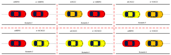
Figure 1.
Six following scenarios of HDVs and CAVs in the traffic stream.
- 2.
- Scenario 2: HDV vehicle following CACC vehicle.
As shown in Figure 1, the front vehicle is a CACC vehicle and the rear HDV vehicle. The way the rear vehicle obtains the front vehicle needs to go through physiological reaction such as driver perception, recognition, and judgment, so the response time is longer. In this scenario, the probability is .
- 3.
- Scenario 3: ACC vehicle following HDV vehicle.
When the CAV follows the HDV vehicle, the front vehicle is the HDV vehicle and the rear vehicle is CAV, the rear vehicle cannot form a car-to-car communication with the front vehicle and the vehicle information cannot be shared in real time, so the CACC vehicle degenerates into the ACC vehicle. As shown in Figure 1, the following mode is in principle the sum of the proportion of CACC and ACC vehicles following HDV vehicles, that is, .
- 4.
- Scenario 4: CACC vehicle following CACC vehicle.
In this case, the rear vehicle and the front vehicle are connected automated vehicles, and the rear vehicle can obtain the position, speed, and acceleration of the front vehicle through vehicle-to-vehicle communication. In this case, the delay of the rear vehicle is the delay in the vehicle-to-vehicle communication process because the vehicle-to-vehicle communication can realize the real-time communication and synchronous driving of the two vehicles. As shown in Figure 1, the car-following mode is in principle the sum of the proportion of CACC and ACC vehicles following CACC vehicles, that is .
- 5.
- Scenario 5: CACC vehicle following ACC vehicle.
As shown in Figure 1, the front connected automated vehicle is degraded to an ACC vehicle by the influence of its front vehicle, and the rear vehicle can still carry out vehicle-to-vehicle communication to obtain information such as the position, speed, and acceleration of the front vehicle. This scenario can realize real-time communication and synchronous driving of the two vehicles. In this scenario, the car-following mode is, in principle, the sum of the proportion of CACC and ACC vehicles following ACC vehicles, that is, .
- 6.
- Scenario 6: HDV vehicle following ACC vehicle.
As shown in Figure 1, the connected automated vehicle is degraded to an ACC vehicle under the influence of the front vehicle, and the HDV vehicle in the rear parking space cannot perform V2V communication. After a physiological reaction such as driver perception, recognition, and judgment, the delay is longer. The proportion of car-following mode in this scenario is .
2.2. HDV/ACC/CACC Car-Following Model
- HDV car-following model
For human-driven vehicles, the widely used intelligent driver model (IDM) is selected. IDM was proposed by Treiber et al. Reference [22], from 2000, has been widely used in the theory and simulation research of HDV car-following models. In this paper, the IDM model is used to simulate the car-following behavior of human-driven vehicles in heterogeneous traffic environments. At this time, the acceleration is:
where represents the speed of vehicle at time . represents the speed difference between the vehicle and the vehicle at time ; represents the headway of vehicle at time ; represents the maximum acceleration parameter of the vehicle, taking ; the free flow speed is ; represents the minimum safe parking spacing, ; represents the safe headway, ; represents comfortable deceleration, ; is long.
- 2.
- ACC car-following model
The PATH laboratory of the University of California, Berkeley, implanted the commercial ACC system into four real vehicles to obtain the trajectory data of the real ACC vehicle, and calibrated the ACC car-following model under the constant inter-vehicle time–distance strategy. The consistency of the calibrated ACC car-following model with the real ACC vehicle in terms of car-following dynamic characteristics [12] is verified. The acceleration of the ACC car-following model is as follows:
where represents the ACC vehicle’ expected workshop time interval parameter, which is ; represents the control coefficient of the spacing error, and the calibration result is . represents the speed difference control coefficient, and the calibration result is .
- 3.
- CACC car-following model
Four real vehicles were implanted into the CACC control system in the PATH laboratory. In order to obtain the trajectory data, the parameters of the CACC control system were calibrated [12,23]. Therefore, the CACC car-following model is as follows:
where represents the speed of vehicle n at time ; represents the control step length of the CACC system, ; represents the error between the actual headway of vehicle at time and the expected headway; represents the differential of with time ; represents the expected workshop distance parameter of the CACC vehicle, ; represents the control coefficient of CACC vehicle spacing error, and the calibration result is 0.45. represents the differential control coefficient of CACC vehicle spacing error, and the calibration result is 0.25.
2.3. Fundamental Diagram Analysis under Heterogeneous Traffic Environment
The traffic flow in a heterogeneous environment is composed of HDVs, CACC, and ACC vehicles. It can be seen from Section 2.1 that the proportion of various vehicles in heterogeneous traffic flow is:
where represents the proportion of CACC vehicles in a heterogeneous traffic environment; represents the proportion of ACC vehicles in a heterogeneous traffic environment; represents the proportion of HDVs in a heterogeneous traffic environment.
It is assumed that the vehicle travels uniformly at an equilibrium speed, . In the process of deriving the traffic flow density in a heterogeneous environment, it is necessary to obtain the road length covered by the heterogeneous traffic flow. Assuming that the total number of vehicles on the road is , the sum of the headway of various vehicles on the road can be obtained:
where represents the headway of HDV; represents the headway of CACC vehicle; represents the headway of ACC vehicle. Therefore,
By the Formulas (5) and (6), the following can be obtained:
Combined with Formulas (1)–(3) and (7), the basic formula of flow-density in heterogeneous traffic environments can be expressed as:
where represents the traffic flow in heterogeneous traffic environments.
According to Formula (8), the heterogeneous traffic environment is determined by the permeability of different CAVs in a mixed traffic flow. Combined with the change of equilibrium speed (), the change of three parameters of traffic flow is calculated every 20% from 0 to 100%. A traffic flow fundamental diagram in heterogeneous environment is obtained when . From Figure 2, it can be seen that with the increase in CAV proportion, the traffic capacity in a heterogeneous traffic environment increases gradually, indicating that the connected automated vehicle has a positive impact on road traffic capacity. It can be seen from Table 2 that when the CAV permeability is 100%, the optimal density is and traffic flow is , which is twice the flow when the CAV permeability is 0.
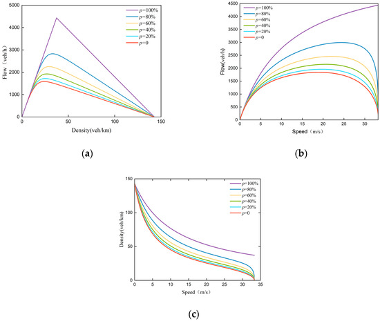
Figure 2.
Traffic flow fundamental diagram of heterogeneous traffic environment (). (a) flow-density; (b) flow-speed; (c) density-speed.
Table 2.
Fundamental graph parameters under different permeabilities in heterogeneous traffic environments.
The maximum traffic capacity and critical density of the road are different under different permeability of connected automated vehicles. The road has higher maximum traffic capacity under high permeability, which indicates that the connected automated vehicles can improve the maximum traffic capacity of the road. However, when the permeability of connected automated vehicles is , the maximum traffic capacity of the road increases with the increase in permeability but the growth rate is slow; when the permeability of connected automated vehicles is greater than 0.6, the maximum capacity of the road is greatly improved with the increase in permeability. The reason is that when the traffic flow changes from single human-driven vehicles to a mixed driving environment of connected automated vehicles and human-driven vehicles, CACC vehicles degenerate into ACC vehicles. In addition, in the process of car-following degradation, ACC vehicles generated by degradation will increase the instability of traffic flow. The fundamental diagram parameters of traffic flow under different permeability in heterogeneous traffic environment are shown in Table 2. The maximum capacity increases by 33.43% when the permeability is 0–60%, and the growth rate is slow. When , the growth rate was significantly accelerated to 2993.80 . It is found that when the permeability is lower than 0.6, human-driven vehicles and ACC vehicles account for the main part of the traffic flow, so the maximum traffic capacity of the road increases slowly. When the permeability exceeds 0.6, CAVs account for the main part of traffic flow, and headway is low, which effectively improves the maximum capacity of the road.
3. Traffic Flow State Analysis Considering Multi-Delay Factors
3.1. Considering Driver Response Time Car-Following Model Update
From the perspective of driver characteristics, the influencing factors of driver response time are decomposed step by step:
- Driver’s physiological attributes such as gender and age;
- Considering that driving experience is the knowledge accumulation of the driver’s long-term driving conditions, the driving age, driving mileage, and driving frequency are selected as the main evaluation indexes to measure the knowledge accumulation;
- The improved driving load assessment method in Reference [24] is used to quantify the driving load of each subject as an indicator of driving load;
- The driver’s expectation is divided into speed expectation, distance expectation, and comfort expectation to reflect the driver’s driving style and driving expectation.
Referring to the value of the driver response time in Reference [24], the range is selected as 0.3~1.3 . In this paper, the data of the real vehicle experiment personnel conform to the normal distribution, and the location of the mean is 0.75. The improved HDV car-following model is obtained from Formula (1):
3.2. Considering CACC and ACC Vehicles’ Communication Delay Time Car-Following Model Update
This section focuses on the linear feedback control in the CACC controller. The advantage of linear control is that the controller has a simple structure, stable operation, and less calculation. By [25], it is found that when the communication delay reaches the delay boundary of the linear controller 0.4 , the linear controller begins to be unstable. Therefore, the linear controller delay is set to 0~0.4 . The improved CACC car-following model is obtained from Formula (3):
Similar to the CACC degraded ACC vehicle, the communication delay is expressed by . The improved ACC car-following model is obtained from Formula (2):
From Formulas (9)–(11), a heterogeneous traffic environment car-following model based on driving response time and communication delay can be obtained:
3.3. Traffic State Analysis
Using the updated car-following model, the traffic flow fundamental diagram considering driver response time and vehicle-to-vehicle communication delay in heterogeneous traffic environment was obtained. As shown in Figure 3, the fundamental diagram without CAV communication delay is shown in the diagram only when the driver’s fastest response time () is considered under a different CAV permeability, which can be compared with the following to show the maximum flow and optimal density.
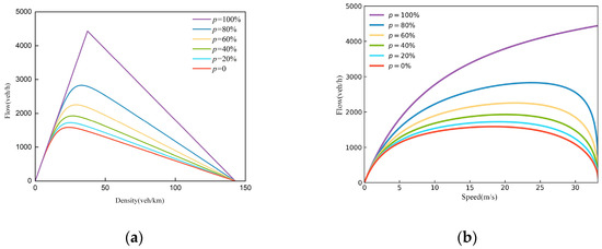
Figure 3.
Updated car-following model fundamental diagram. (a) flow-density; (b) flow-speed; (c) density-speed.
It can be seen from Figure 4 and Figure 5 that with the increase in driver response time or communication delay of CACC linear controller, the maximum capacity under a different CAV permeability is decreasing. When permeability drops to 40%, the maximum flow of CACC vehicles changes little with the increase in communication delay. With the increasing permeability of CAVs, the impact of vehicle-to-vehicle communication technology on heterogeneous traffic flow is more obvious. In the future, the impact of communication delay on headway can be compared under different connected automated vehicles’ communication control systems.
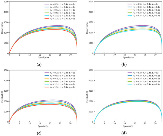
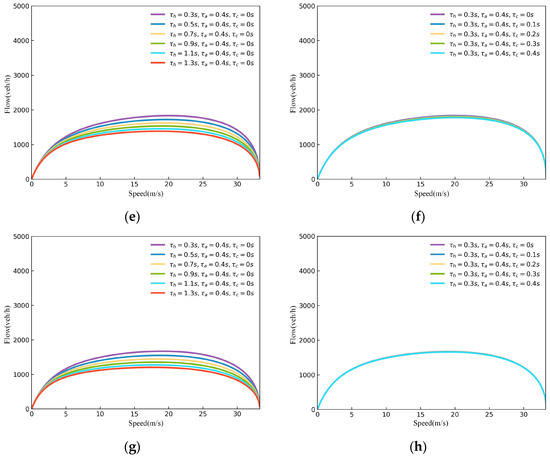
Figure 4.
The flow-speed diagram considering the driver response time and the communication delay of V2V communication linear controller (a) , driver response change flow-speed diagram; (b) , communication delay flow-speed diagram; (c) , driver response change flow-speed diagram; (d) , communication delay flow-speed diagram; (e) , driver response change flow-speed diagram; (f) , communication delay flow-speed diagram; (g) , driver response change flow-speed diagram; (h) , communication delay flow-speed diagram.
Figure 5.
The density-speed diagram considering the driver response time and the communication delay of V2V communication linear controller (a) , driver response change density-speed diagram; (b) , communication delay density-speed diagram; (c) , driver response change density -speed diagram; (d) , communication delay density-speed diagram; (e) , driver response change density-speed diagram; (f) , communication delay density-speed diagram; (g) , driver response change density -speed diagram; (h) , communication delay density-speed diagram.
4. Model Illustration
4.1. Simulation Environment Settings
In this section, a simulation experiment is designed to verify the fundamental diagram model of this paper. Specifically, a mixed traffic flow simulation environment is constructed in the SUMO software, and traffic flow, density, and speed data are collected by the software. Among them, the simulation section is designed as a decagonal loop connected by ten single lanes with a length of 1 km, as shown in Figure 6.
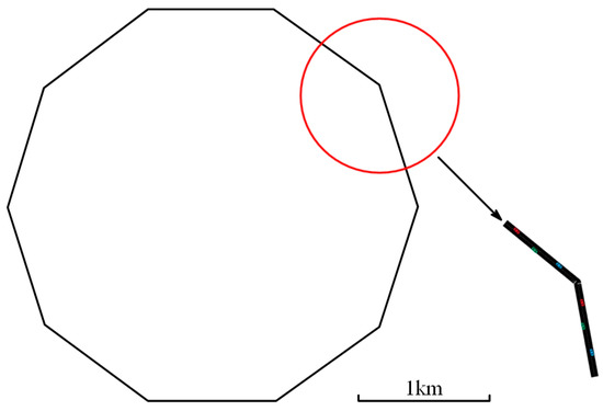
Figure 6.
Simulation road network settings.
The simulation does not consider the vehicle lane-changing behavior. The updated car-following model is reflected in SUMO by the change of HDV/ACC/CACC safety headway, and the remaining car-following model parameters use the parameters in Formulas (1)–(3). The maximum speed of the road section is set to 33.3 . At the same time, in order to obtain the flow-density scatter point when the density is large, the deceleration interference is performed on the specified road section when the simulation runs to a certain time, and the vehicle speed on the road section is reduced to 1 . Data detection is performed on each road section (10 in total). The detection frequency is set to 2 min, and the flow is calculated from the obtained data. SUMO simulation parameter setting reference Table 3.
Table 3.
SUMO simulation parameter setting.
4.2. Analysis of Simulation Results
Through the data collected in the simulation experiment, the relationship between traffic flow and density under CAV permeability is obtained (), as shown in Figure 7. Furthermore, the relationship between traffic flow and density () considering the communication delay of CACC vehicle linear controller in the permeability is shown in Figure 8.
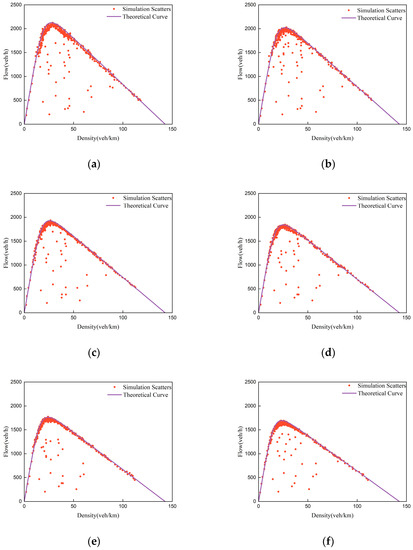
Figure 7.
The simulation results considering the driver response time change () (a) ; (b) ; (c) ; (d) ; (e) ; (f) .
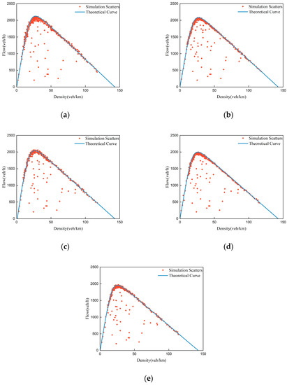
Figure 8.
Simulation results considering the change of communication delay of V2V communication linear controller () (a) ; (b) ; (c) ; (d) ; (e) .
The data points obtained by the SUMO simulation are basically distributed around the theoretical curve, which proves the validity and correctness of the fundamental diagram model. From the simulation scatter distribution of Figure 7 and Figure 8, it can be seen that with the increase in response time and communication delay, the maximum flow obtained by simulation gradually decreases and the flow-density scatter diagram obtained after the traffic flow that reaches the equilibrium state is on both sides of the corresponding theoretical curve. This is highly consistent with the theoretical curve (abnormal points are mainly generated when the traffic flow is in a non-equilibrium state and speed limit), which proves the rationality and accuracy of using the theoretical model to deal with the delay.
5. Conclusions
In this paper, the proportion of vehicles in six different scenarios of car-following fleet in a heterogeneous traffic environment was analyzed. Then the car-following models of HDV, CACC, and ACC vehicles are analyzed. On this basis, fundamental diagram model of heterogeneous traffic flow is derived, and then the car-following model is updated by considering the driver response time and V2V communication delay. Finally, the simulation experiment is designed in SUMO to verify model effectiveness in dealing with driver response time and V2V communication delay. The following conclusions can be drawn from the analysis:
- When the permeability of CAVs is greater than 0.6, it has a positive impact on the maximum flow of traffic flow in a heterogeneous environment. With the increase in the proportion of connected automated vehicles, the maximum flow and optimal density of mixed traffic flow gradually increase, which can effectively improve road capacity and help solve traffic congestion.
- Driver response time and vehicle-to-vehicle communication delay have a negative impact on the maximum flow of a heterogeneous traffic flow. As the delay increases, the maximum flow and optimal density of a heterogeneous traffic flow gradually decrease. However, when the permeability is lower than 0.4, the impact on CAVs is small.
- Based on the data collected from the simulation experiment, the flow-density scatter plot obtained after the traffic flow reaches the equilibrium state is on both sides of the corresponding theoretical curve, which is highly consistent with the theoretical curve. It proves the rationality and accuracy of using the updated car-following model to deal with driver response time and vehicle-to-vehicle communication delay.
In this paper, the flow-speed-density variation law of multi-delay traffic flow is considered, and the accuracy of the fundamental diagram model is improved by using the updated car-following model. However, only the linear communication controller system is considered in the process of the vehicle-to-vehicle communication of CAVs. Therefore, the communication delay compensation method proposed by model predictive control (MPC) can be used to study the vehicle stability under different controller conditions and broaden the research depth.
Author Contributions
Conceptualization, S.G. and C.M.; methodology, J.W. and C.M.; software, S.G. and C.M.; investigation, S.G. and C.M.; writing—original draft preparation, S.G. and C.M.; writing—review and editing, S.G., C.M. and J.W.; visualization, C.M. and S.G.; supervision, C.M. All authors have read and agreed to the published version of the manuscript.
Funding
This research was funded by the National Natural Science Foundation of China under Grant No.52172338. Shaanxi Province 2023 Natural Science Basic Research Plan Project under Grant No.2023-JC-YB-332.
Institutional Review Board Statement
Not applicable.
Informed Consent Statement
Not applicable.
Data Availability Statement
Not applicable.
Conflicts of Interest
The authors declare no conflict of interest.
References
- Bansal, P.; Kockelman, K.M. Forecasting Americans′ Long-term Adoption of Connected and Autonomous Vehicle Technologies. Transp. Res. Part A Policy Pract. 2017, 95, 49–63. [Google Scholar] [CrossRef]
- Wang, Y.; Xu, R.; Zhang, K. A Car-Following Model for Mixed Traffic Flows in Intelligent Connected Vehicle Environment Considering Driver Response Characteristics. Sustainability 2022, 14, 11010. [Google Scholar] [CrossRef]
- Qin, Y.; Wang, H.; Wang, W.; Wan, Q. Fundamental Diagram Model of Heterogeneous Traffic Flow Mixed with Cooperative Adaptive Cruise Control Vehicles and Adaptive Cruise Control Vehicles. China J. Highw. Transp. 2017, 30, 127–136. [Google Scholar]
- Wang, X.; Liu, S.; Shi, H.; Xiang, H.; Zhang, Y.; He, G.; Wang, H. Impact of Penetrations of Connected automated vehicles on Lane Utilization Ratio. Sustainability 2022, 14, 474. [Google Scholar] [CrossRef]
- Lunge, A.; Borkar, P. A Review on Improving Traffic Flow Using Cooperative Adaptive Cruise Control System. In Proceedings of the 2015 2nd International Conference on Electronics and Communication Systems, Coimbatore, India, 26–27 February 2015. [Google Scholar]
- Talebpour, A.; Mahmassani, H.S. Influence of Connected and Autonomous Vehicles on Traffic Flow Stability and Throughput. Transp. Res. Part C Emerg. Technol. 2016, 71, 143–163. [Google Scholar] [CrossRef]
- Chang, X.; Li, H.; Rong, J.; Qin, L.; Yang, Y. Analysis on Fundamental Diagram Model for Mixed Traffic Flow with Connected Vehicle Platoons. J. Southeast Univ. 2020, 50, 782–788. [Google Scholar]
- Levin, M.W.; Boyles, S.D. A Multiclass Cell Transmission Model for Shared Human and Autonomous Vehicle Roads. Transp. Res. Part C Emerg. Technol. 2016, 62, 103–116. [Google Scholar] [CrossRef]
- Xu, T.; Yao, Z.; Jiang, Y. The Fundamental Diagram Model Considering the Influence of Reaction Time of Mixed Traffic Flow of Connected Automated Vehicles. J. Highw. Transp. Res. Dev. 2020, 37, 108–117. [Google Scholar]
- Arem, B.V.; Driel, C.; Visser, R. The Impact of Cooperative Adaptive Cruise Control on Traffic-Flow Characteristics. IEEE Trans. Intell. Transp Syst. 2006, 7, 429–436. [Google Scholar] [CrossRef]
- Vabder, W.J.; Shladover, S.; Kourjanskaia, N.; Miller, M. Modeling Effects of Driver Control Assistance Systems on Traffic. Transp. Res. Rec. 2001, 1748, 167–174. [Google Scholar]
- Milanés, V.; Shladover, S.E. Modeling Cooperative and Autonomous Adaptive Cruise Control Dynamic Responses Using Experimental Data. Transp. Res. Part C Emerg. Technol. 2014, 48, 285–300. [Google Scholar] [CrossRef]
- Lv, N.; Ren, Z.; Duan, Z.; Luo, Y. Analysis of Driving Behavior Characteristics of Drivers in Near-crash Events. China Saf. Sci. J. 2017, 27, 19–24. [Google Scholar]
- Shevtsova, A.; Novikov, I.; Borovskoy, A. Research of Influence of Time of Reaction of the Driver on the Calculation of the Capacity of The Highway. Transp. Probl. 2015, 10, 53–59. [Google Scholar] [CrossRef]
- Sena, P.; D’amore, M.; Brandimonte, M.A.; Squitieri, R.; Fiorentino, A. Experimental Framework for Simulators to Study Driver Cognitive Distraction: Brake Reaction Time in Different Levels of Arousal. Transp. Res. Procedia 2016, 14, 4410–4419. [Google Scholar] [CrossRef]
- Darbha, S.; Konduri, S.; Pagilla, P.R. Benefits of V2V Communication for Autonomous and Connected Vehicles. IEEE Trans. Intell. Transp. Syst. 2018, 20, 1954–1963. [Google Scholar] [CrossRef]
- Naus, G.; Vugts, R.; Ploeg, J.; van de Molengraft, M.; Steinbuch, M. String-Stable CACC Design and Experimental Validation: A Frequency-Domain Approach. IEEE Trans. Veh. Technol. 2010, 59, 4268–4279. [Google Scholar] [CrossRef]
- Dey, K.C.; Yan, L.; Wang, X.; Shen, H.; Chowdhury, M.; Yu, L.; Qiu, C.; Soundararaj, V. A Review of Communication, Driver Characteristics, and Controls Aspects of Cooperative Adaptive Cruise Control (CACC). IEEE Trans. Intell. Transp. 2016, 17, 491–509. [Google Scholar] [CrossRef]
- Rajamani, R.; Zhu, C. Semi-autonomous Adaptive Cruise Control Systems. In Proceedings of the American Control Conference, San Diego, CA, USA, 2–4 June 1999. [Google Scholar]
- Xu, Z.; Li, J.; Zhao, X.; Li, L.; Wang, Z.; Tong, X.; Tian, B.; Hou, J.; Wang, G.; Zhang, Q. A Review on Intelligent Road and Its Related Key Technologies. China J. Highw. Transp. 2019, 32, 1–24. [Google Scholar]
- Ma, Y.; Li, Z.; Malekian, R.; Zhang, R.; Song, X.; Sotelo, M.A. Hierarchical Fuzzy Logic-based Variable Structure Control for Vehicles Platooning. IEEE Trans. Intell. Transp. 2019, 20, 1329–1340. [Google Scholar] [CrossRef]
- Treiber, M.; Hennecke, A.; Helbing, D. Congested Traffic States in Empirical Observations and Microscopic Simulations. Phys. Rev. E 2000, 62, 1805–1824. [Google Scholar] [CrossRef]
- Milanés, V.; Shladover, S.E.; Spring, J.; Nowakowski, C.; Kawazoe, H.; Nakamura, M. Cooperative Adaptive Cruise Control in Real Traffic Situations. IEEE Trans. Intell. Transp. 2014, 15, 296–305. [Google Scholar] [CrossRef]
- Guo, B.; Jin, L.; Shi, J.; Zhang, S. A Risky Prediction Model of Driving Behaviors: Especially for Cognitive Distracted Driving Behaviors. In Proceedings of the 2020 4th CAA International Conference on Vehicular Control and Intelligence (CVCI), Hangzhou, China, 18–20 December 2020. [Google Scholar]
- Tian, B.; Yao, K.; Wang, Z.; Gu, G.; Xu, Z.; Zhao, X.; Jing, J. Communication Delay Compensation Method of CACC Platooning System Based on Model Predictive Control. J. Traffic Transp. Eng. 2022, 22, 361–381. [Google Scholar]


Disclaimer/Publisher’s Note: The statements, opinions and data contained in all publications are solely those of the individual author(s) and contributor(s) and not of MDPI and/or the editor(s). MDPI and/or the editor(s) disclaim responsibility for any injury to people or property resulting from any ideas, methods, instructions or products referred to in the content. |
© 2023 by the authors. Licensee MDPI, Basel, Switzerland. This article is an open access article distributed under the terms and conditions of the Creative Commons Attribution (CC BY) license (https://creativecommons.org/licenses/by/4.0/).