Insights into the Distribution of Soil Organic Carbon in the Maoershan Mountains, Guangxi Province, China: The Role of Environmental Factors

Abstract

The forest ecosystem is the largest carbon reservoir in the terrestrial ecosystem, with soil organic carbon (SOC) being its most important component. How does the distribution of forest SOC distribution change under the influence of regional location, forest succession, human activities, and soil depth? It is the basis for understanding and evaluating the value of forest SOC reservoirs and improving the function of forest soil carbon sinks. In this paper, soil organic carbon concentrations (SOCCs) and environmental factors were measured by setting 14 experimental plots and 42 soil sampling sites in different forest communities and different elevations in the Maoershan Mountains. The redundancy analysis (RDA) method was used to study the relationship between SOC distribution and external factors. The results show that SOC distribution was sensitive to elevation, forest community, and soil layer. It had obvious surface aggregation characteristics and increased significantly with the increase in elevation. Among them, SOCCs increase by 1.80 g/kg with every 100 m increase in elevation, and that decreased by 5.43 g/kg with every 10 cm increase in soil depth. The SOC distribution in natural forests is greater than that in plantations, and the spatial variation in SOC distribution in plantations is higher due to the effect of cutting and utilization. SOC distribution is the result of many environmental factors. The response of SOC distribution to the forest community indicates that the development of plantations into natural forests will increase SOC, and excessive interference with forests will aggravate SOC emissions. Therefore, strengthening the protection of natural forests, restoring secondary forests, and implementing scientific and reasonable plantation management are important measures for improving the SOC reservoir’s function.

1. Introduction

Carbon is an essential component of the terrestrial ecosystem [1], and the biological cycling processes of many elements are closely related to carbon [2]. The terrestrial ecosystem is a huge carbon pool, which is important in regulating the Earth’s climate and supporting life on land [3]. Soils are large reservoirs of organic carbon and play a significant role in its accumulation and storage [4]. Soil organic carbon (SOC) is composed of active carbon and non-active carbon, and it is an indicator when evaluating soil quality [5]. SOC is mostly present in the first 0–40 cm. The global SOC pool is 2–3 times that of the terrestrial vegetation carbon pool [6], and the SOC at 1 m soil depth is 1.5 times that of the total existing biomass (natural vegetation and crops) [7]. The forest ecosystem is the main body of the terrestrial ecosystem, and forest soil organic carbon (FSOC) accounts for approximately 16–26% of the global terrestrial ecosystem’s carbon storage [8,9], which is more than 73% of global SOC [10]. Additionally, it is about 2.7 times that of forest biomass carbon [11].

Since the 1980s, the study of the carbon cycle has become an important research focus in the field of environmental ecology under the influence of global warming [12]. Among them, the study on the relationship between FSOC and environmental change is mainly based on the quantitative analysis and model simulation of experimental observation. Generally, analysis of variance (ANOVA), redundancy analysis (RDA), and coefficient of variation (CV) statistics are mainly used to explore the relationship between FSOC and environmental change. ANOVA is mainly used to test the significance of the difference between two or more samples and to find out the factors that have a significant influence on the research object, the interaction between the factors, and the degree of significance of the influence. The key to ANOVA is to analyze and decompose the factors causing a change in the test results and conduct an F test (p = 0.05) to determine whether there are differences in the influence of experimental treatments on the results. RDA can effectively perform statistical tests on multiple environmental indicators and evaluate the relationship between one or a set of variables and another set of variable data from the perspective of statistics [13]. The key to RDA is to filter the characteristics of environmental factors, simplify the number of variables, and visually reflect the relationship between the response variable and explanatory variable on the same axis so as to obtain the relationship between environmental factors and SOC [13]. The coefficient of variation (CV) is a parameter used to compare the dispersion degree of two groups of experimental data, which is not only affected by the dispersion degree of experimental data but also by the average level of experimental data. The closer the CV is to 1, the more uneven the experimental data will be, and the closer the CV is to 0, the more uniform the experimental data will be.

A large number of studies have shown that extreme weather in some regions is associated with a loss of forest area and a decline in soil health [14]. FSOC is a main source and sink of atmospheric CO₂, greatly influenced by parent rock and vegetation, and sensitive to climate change and human interference, playing an irreplaceable role in the global carbon cycle [15]. Natural climate change affects the type and quantity of SOC by affecting plant growth, biomass accumulation, and litter decomposition [16]. Forests absorb CO₂ through photosynthesis and release it back into the atmosphere in various forms of respiration or disturbance, thus forming the terrestrial ecosystem carbon cycle of atmosphere–vegetation–soil. The distribution of FSOC is the result of forest and environmental factors and climate change. Elevation has a significant impact on the distribution of SOC, but with the increase in soil depth, elevation has a smaller impact on the distribution of SOC [17]. Changes in the SOC reservoir are caused by soil animal activities and soil microenvironment changes [18]. Different land uses have an influence on the uncertainty of SOC storage [19]. The conversion of agricultural land into forestland significantly increases soil carbon storage [20]. Soil disturbance by human activities affects SOC emissions and has a great impact on global ecological environment changes [21].

In recent years, increasing attention has been paid to forest carbon storage and its dynamic change as global environmental problems become increasingly prominent and the understanding of the forest’s ecological role is enhanced. Research regarding the distribution of SOC and its environmental ecological effects mostly focuses on the impacts of natural and human factors, such as climate, vegetation, physical and chemical factors, human cultivation, land use, irrigation, and so on [19,22]. FSOC is sensitive to climate fluctuations and is easily influenced by biological and non-biological factors, such as vegetation cover types, land use types, and environmental conditions. It also regulates soil physical, chemical, and biological characteristics, and is an important indicator by which to evaluate the absorption and fixation of CO₂ in forest ecosystems [23,24]. The proportion of SOC in global forests compared to SOC in land is approximately 16–39% [8,11,25,26,27]. This leads to uncertainty and inconsistency in carbon trading negotiations and affecting inter-regional CO₂ emission control. Therefore, studying the spatial distribution of FSOC and its response to environmental factors in typical regions can enable a prediction of the trend of climate change and reveal the effects of human activities on SOC emissions [28]. It can also enhances awareness of the importance of maintaining forest carbon sequestration [29], provides a theoretical basis for forest carbon sink function assessment and carbon sink management [30], and offers scientific and technical support for the realization of the “carbon peak and carbon neutrality” strategy.

Subtropical forests in China are unique among global forest ecosystems, with obviously heterogeneous SOC distribution due to forest succession and anthropogenic activities, which makes it difficult to evaluate the ecological function and service value of forest soil carbon. In this paper, we hypothesize that SOC distributions among different forest communities have quantitative rules. Taking the Maoershan Mountains, the highest peak in South China and the most representative and well-preserved natural forests in the mid-subtropical region, as the research object, we study the relationship between SOC distribution and forest community, elevation, and soil depth in order to solve the following problems:

(1)

Are there significant differences in SOC distribution between different forest communities and elevations? Can a unified index be used to evaluate forest soil carbon storage?

(2)

Which of the topographic factors, soil factors, or forest factors contributed more to the difference in SOC distribution?

(3)

Will the development of plantations into natural forests improve the storage capacity of SOC?

This study provides a scientific basis for evaluating the ecological function and service value of forest SOC, rationally regulating the distribution of forest communities, improving the function of forest soil carbon pool and carbon sink, and effectively controlling CO₂ emission.

2. Materials and Methods

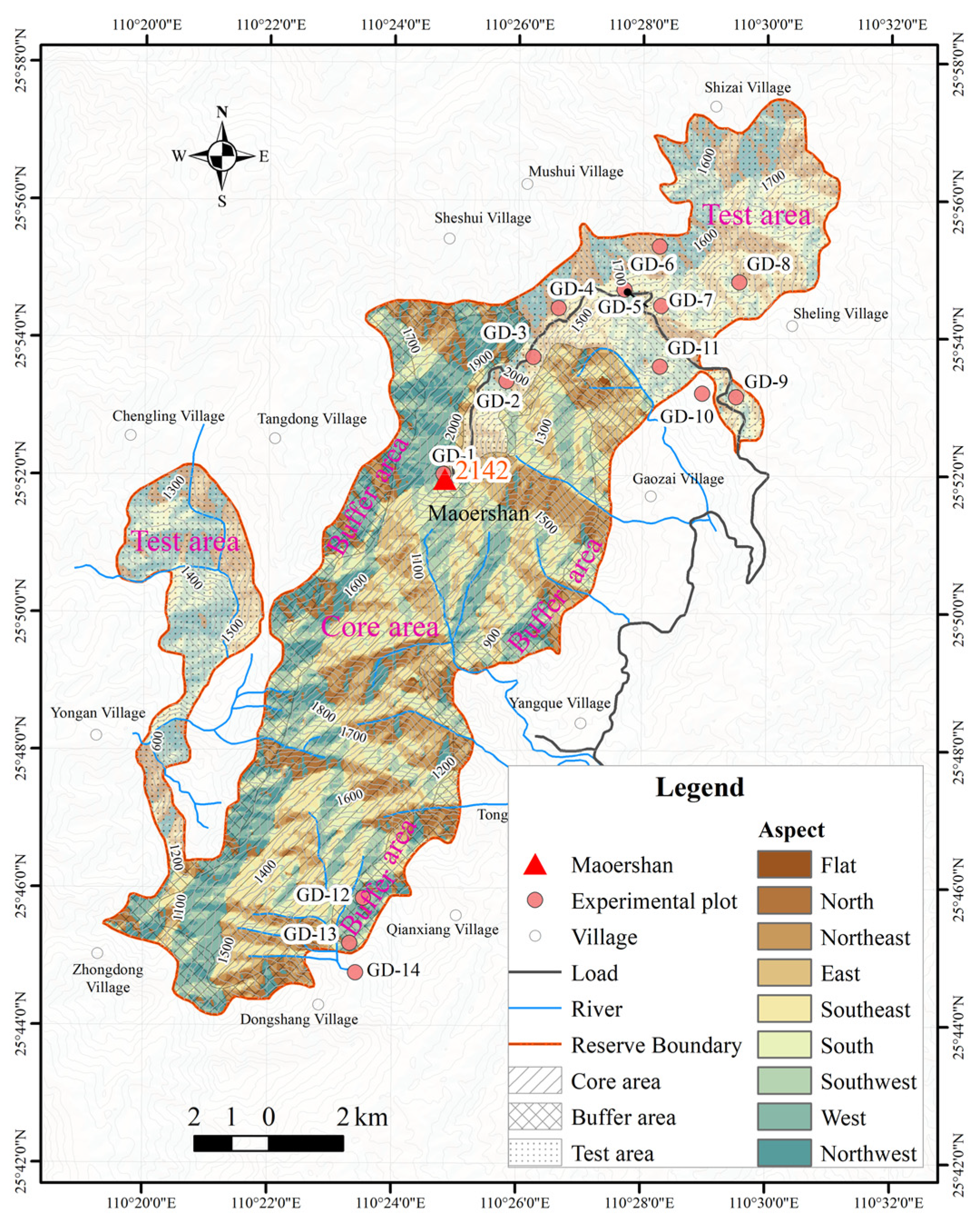
2.1. Study Sites

The Maoershan Mountains (109°36′55′′~111°29′12′′ E, 24°15′23′′~26°23′19′′ N) are located in the north of Guilin, Guangxi Province, and belong to the Yuechengling Mountain system of the Nanling Mountain chain (Figure 1). These have a northeast–southwest trend, and the elevation of their highest peak is 2141.5 m above sea level, making this the highest peak in Southern China. The relative elevation is 1862 m. The region has obvious subtropical mountain climate characteristics affected by geographical environmental factors such as elevation, terrain, and forest. The average annual temperature is 12.8 °C, the average annual relative humidity is 92%, and the average annual rainfall is 2509.1 mm [31]. The geomorphology is divided into erosion and denudation, and the soil parent material is granite [32,33]. Forest types and soil types are distributed zonally along the elevation, and the typical zonal forest type is an evergreen broad-leaved forest (

Table 1. Distribution of forest vegetation types and soil types along elevation in the Maoershan Mountains.

Elevation	Forest Vegetation Types	Soil Types [32,33]
<400 m	1. Phyllostachys Edulis forests (plantations) 2. Cunninghamia lanceolate forests (plantations) 3. Shrub forests (secondary forest)	Hilly red soil
400–700 m	1. Deciduous broad-leaved forest (secondary forest) 2. Phyllostachys Edulis forests (plantations) 3. Cunninghamia lanceolate forests (plantations) 4. Shrub forests (secondary forest)	Mountain yellow–red soil
700–1200 m	1. Evergreen broad-leaved forest (secondary forest) 2. Deciduous broad-leaved forest (secondary forest) 3. Phyllostachys Edulis forests (plantations) 4. Shrub forests (secondary forest)	Mountain yellow soil
1200–1800 m	1. Evergreen deciduous broad-leaved mixed forest (secondary forest) 2. Evergreen broad-leaved forest (secondary forest) 3. Shrub forests (secondary forest) 4. Bamboo forests (secondary forest)	Mountain brown soil Mountain yellow–brown soil
1800–2000 m	1. Mountain top coppice (secondary forest) 2. Shrub forests (secondary forest)	Peat soil
>2000 m	Mountain meadow	Hilltop dwarf forest soil

). The main forest communities are shrub forests (SF), Cyclobalanopsis stewardiana forests (CSF), Fagus longipetiolata forests (FLF), Schima superba forests (SSF), Phyllostachys edulis forests (PEF), Cunninghamia lanceolata forests (CLF), and Pinus massoniana forests (PMF) [34,35].

2.2. Investigation of Environmental Factors and Soil Sample Collection

Forest soil shows significant spatial variability due to surface fluctuation, vegetation distribution, and forest management activities [36,37]. According to the “Method for Long-Term Positioning and Observation of Forest Ecosystems” (GB/T 33027-2016 [38]), zonal forest communities were selected for each elevation and separated by at least 200 m, and three 20 × 20 m² experiment plots were set up according to three repeated requirements. The environmental factors, such as elevation (ELE), slope gradient (SG), and slope position (SP), and forest vegetation factors, such as stand age (SA), stand density (SD), and canopy coverage (CC), were measured in detail. Three 5 × 5 m² shrub quadrat and five 1 × 1 m² herb quadrats were set up in each experiment plot. The aboveground biomass of shrubs and herbs was measured by the sample method (shrub) and the harvest method (herb). A total of 14 experiment plots were set up.

In each experiment plot, 3 soil sampling points (there are 42 sampling points) were set outward from the center, and soil profiles with a width of 0.8–1.0 m were excavated with a spade. Soil samples were collected layer-by-layer from 0 to 15 cm, 15 to 30 cm, 30 to 45 cm, and 45 to 60 cm, and the profile morphology was observed and described. Combined with the soil sampling profile, the excavation continued to the bedrock. The distance from the ground to the bedrock was used as the soil thickness (ST), which was measured with a steel ruler with an accuracy of 1 mm. The basic information about the experiment plots is shown in

Table 2. Basic information of experiment plots.

Forest Community	Elevation(m)	Slope Position	Slope Gradient (°)	Soil Depth (cm)	Soil pH	Soil Bulk Density (SBD, g/kg)	Stand Density (Plant/hm2)/Canopy Coverage (%)	Name of Dominant Tree Species
SF	2120	Upper	47	85	4.2	0.960	70	Fargesia spathacea franch; Buxus sinica (Rehd. et Wils.) Cheng
SF	2005	Middle	52	85	4.5	1.030	75	Fargesia spathacea franch; Buxus sinica (Rehd. et Wils.) Cheng
CSF	1950	Lower	20	150	4.6	0.690	1125	Cyclobalanopsis stewardiana (A. Camus) Y. C. Hsu et H. W. Jen; Prunus spinulosa, Camellia pitardii
FLF	1810	Upper	48	133	4.4	0.920	1100	Fagus longipetiolata Seem; Fargesia spathacea franch
SF	1580	Upper	55	50	4.2	0.900	60	Fargesia spathacea franch; Buxus sinica (Rehd. et Wils.) Cheng
FLF	1400	Upper	52	120	4.5	0.890	1100	Fagus longipetiolata Seem
SSF	1280	Upper	57	85	4.7	0.990	1600	Schima superba Gardn. et Champ; Manglietia fordiana Oliv
SF	1240	Upper	54	55	4.4	0.910	72	Fargesia spathacea franch
PEF	1210	Lower	47	60	5.0	0.954	4300	Phyllostachys pubescens
CLF	1210	Middle	48	60	4.9	1.093	2850	Cunninghamia lanceolata
SF	1127	Upper	48	60	4.1	0.900	75	Fargesia spathacea franch
PMF	890	Middle	50	80	4.5	0.930	1232	Pinus massoniana
CLF	640	Middle	47	115	4.4	0.820	3050	Cunninghamia lanceolata
PEF	460	Middle	50	110	4.4	0.780	4122	Phyllostachys pubescens

SSF, Schima superba forests; CSF, Cyclobalanopsis stewardiana forests; FLF, Fagus longipetiolata forests; PMF, Pinus massoniana forests; PEF, Phyllostachys edulis forests; CLF, Cunninghamia lanceolata forests; SF, shrub forests.

.

2.3. Determination of Soil Samples

According to the “Laboratory methods of soil analysis” [39], the soil samples collected at each soil sampling site were dried and mixed evenly. Two samples were taken using the quarto method. The samples were sieved through a 2 mm screen after stones and plant roots were removed. Soil samples were air dried and then used to measure pH and SOC. The SOC concentrations were analyzed using the potassium oxidation method (H₂SO₄–K₂Cr₂O₇) of Walkey and Black [40]. Soil bulk density (SBD) was determined by the ring knife method, and soil pH in H₂O (1:2.5, soil/water ratio) was determined with an FE20K pH meter (Mettler Toledo, Switzerland).

2.4. Data Processing

2.4.1. Calculation of Soil Organic Carbon Concentrations (SOCCs) and Soil Organic Carbon Reserves (SOCRs)

In this study, SOCCs and soil organic carbon reserves (SOCRs) were used to indicate the status of SOC. The SOCC was determined per soil sample (unit: g/kg) [39]. The SOCR denotes the storage of SOC per unit area of a certain soil layer (unit: t/hm²) and is calculated according to Formula (1):

ρ = β × μ × h × (1 − α)/10,

(1)

where ρ is the SOCR of a certain soil layer (t/hm²), β is the actual measured SOCC of a certain soil layer (g/kg), μ is the SBD of a certain soil layer (g/cm³), h is the thickness of a certain soil layer (cm), α is the volume percentage of gravel with diameter > 2 mm of a certain soil layer, and α = 0 because samples with diameters less than 2 mm were selected.

2.4.2. Analysis of Variance (ANOVA)

In this study, the experimental treatments were different environmental conditions (forest type, elevation, or soil layer), and the experimental results were SOCCs and SOCRs. SPSS 23.0 was used for ANOVA and Multiple Comparisons (p = 0.05). The results of the ANOVA were used to determine whether there are significant differences in the SOCCs and SOCRs among different forest types, elevations, or soil layers. If Sig. < 0.05, it indicates that there are significant differences in the SOCCs and SOCRs among different forest types, elevations, or soil layers, which indicates that changes in forest types, elevations, or soil layers have significant effects on the spatial distribution of SOC, and Sig. > 0.05 indicates that the impact is small. According to the results of Multiple Comparisons, we can determine whether there are significant differences in the SOCCs and SOCRs between pairwise forest types, elevations, or soil layers, and identify specific forest types, elevations, or soil layers that have a significant impact on SOC distribution. Sig. < 0.05 indicates that there are significant differences between pairwise forest types, elevations, or soil layers. Sig. > 0.05 indicates that there is no significant difference.

2.4.3. Redundancy Analysis (RDA)

In this study, the SOCCs and SOCRs were set as the “response variable”, and the environmental factors such as forest type (FT), elevation (ELE), and soil thickness (ST) were set as the “explanation variables” according to the basic principle of RDA. CANOCO 5 was used for RDA to determine the explainability of environmental factors to the spatial variation in SOC.

2.4.4. Coefficient of Variation (CV)

The coefficient of variation (CV) is a parameter used to compare the dispersion degree of two groups of experimental data, which is not only affected by the dispersion degree of experimental data, but also affected by the average level of experimental data. The closer the CV is to 1, the more uneven the experimental data will be, and the closer the CV is to 0, the more uniform the experimental data will be. In this study, the experimental data are SOCCs and SOCRs under different environmental conditions. The CV was used to reflect the degree of variation in the SOCCs and SOCRs. The closer the CV is to 1.0, the more uneven the SOC distribution is, while the closer CV is to 0.0, the more uniform the SOC distribution is. The CV is calculated using Formula (2):

$$\mathrm{CV}=\mathsf{\sigma }/\mathsf{\mu }$$

(2)

where σ is the standard deviation; μ is the mean.

All analyses and visualizations were conducted in R-4.2.3 (R Project for Statistical Computing; http://www.R-project.org, accessed on 15 March 2023.) with Rstudio.

3. Results and Analysis

3.1. Spatial Variation in SOC

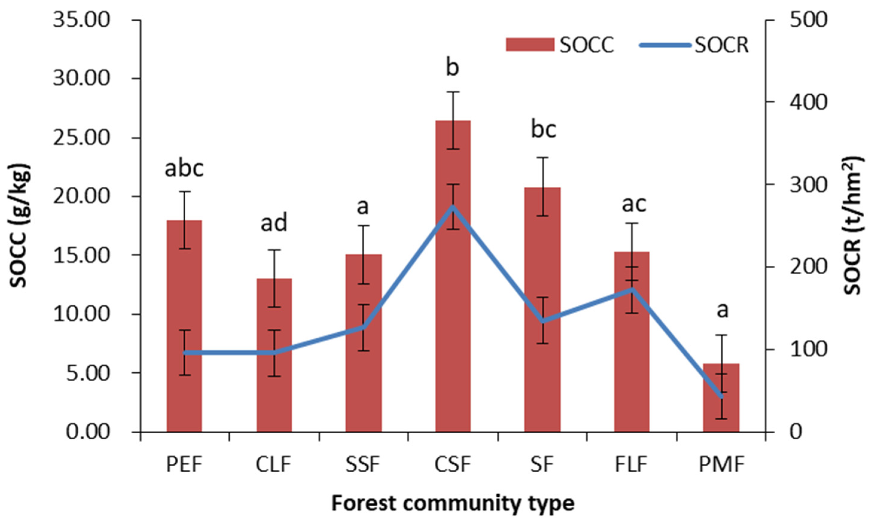
3.1.1. Horizontal Distribution of SOC

Figure 2 shows that there was obvious spatial heterogeneity in the SOC distributions of different forest communities, the SOCC and SOCR varied greatly, and the SOCC was 5.83–26.43 g/kg, while the SOCR was 43.39–273.15 t/hm². The average SOCC in the different forest communities was 17.61 g/kg, and the order from high to low was CSF > SF > PEF > FLF > SSF > CLF > PMF. The average SOCR in different forest communities was 132.10 t/hm², and the order was CSF > FLF > SF > SSF > PEF > CLF > PMF. The order of the SOCC and SOCR from high to low was obviously different. The results of the ANOVA using SPSS 23.0 show that there were significant differences in the SOCC among different forest communities (p = 0.04 < 0.05); the multiple comparisons show that there were significant differences between CSF and CLF; SSF, FLF, PMF, and SF; and PMF, CLF, and SSF (p < 0.05).

Figure 3 shows that the SOC distribution in the Maoershan Mountains was uneven, and the CV of the SOCC was 0.73. The SOC distribution in FLF was very uneven, with the highest CV of the SOCC (0.92), and the SOC distribution in CSF was the most uniform, with the lowest CV of the SOCC (0.27). CSF is natural forests and FLF is plantations. The results show that the SOC distribution in the natural forests of the Maoershan Mountains was higher than that in plantations. Due to the influence of forest management activities, the variation in SOC distribution in the plantations was high, indicating that the anthropogenic disturbance had a great impact on SOC distribution.

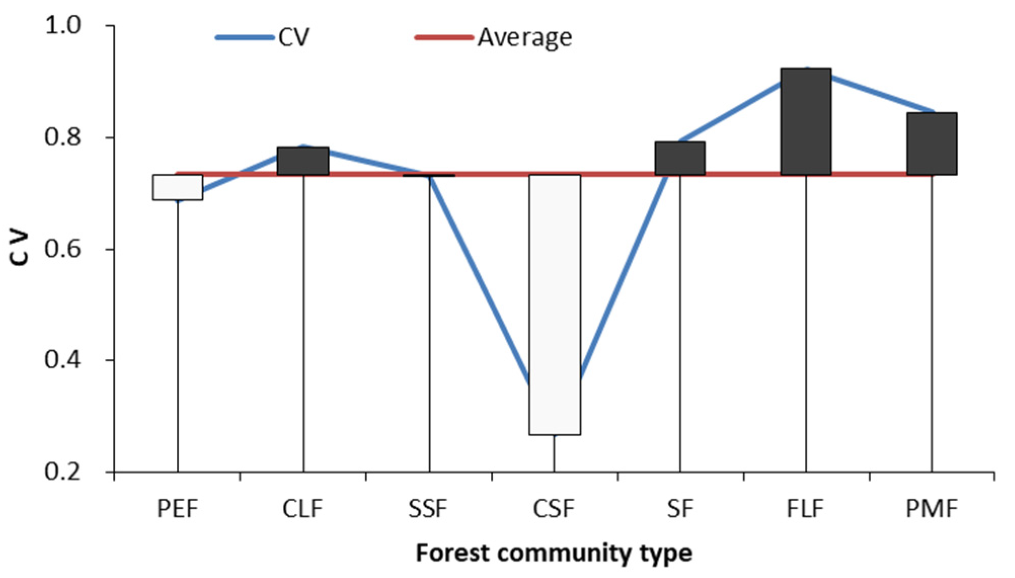
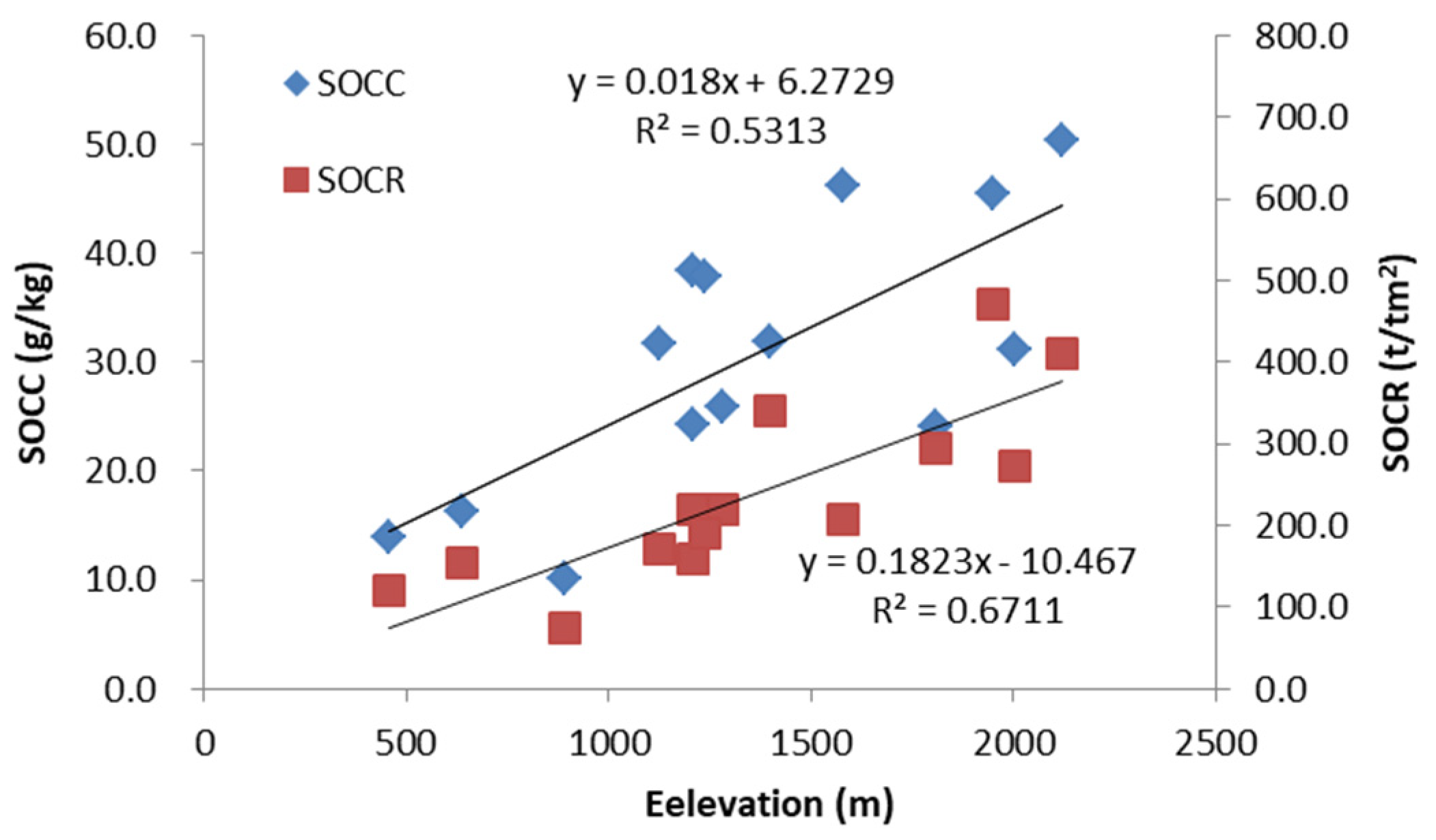
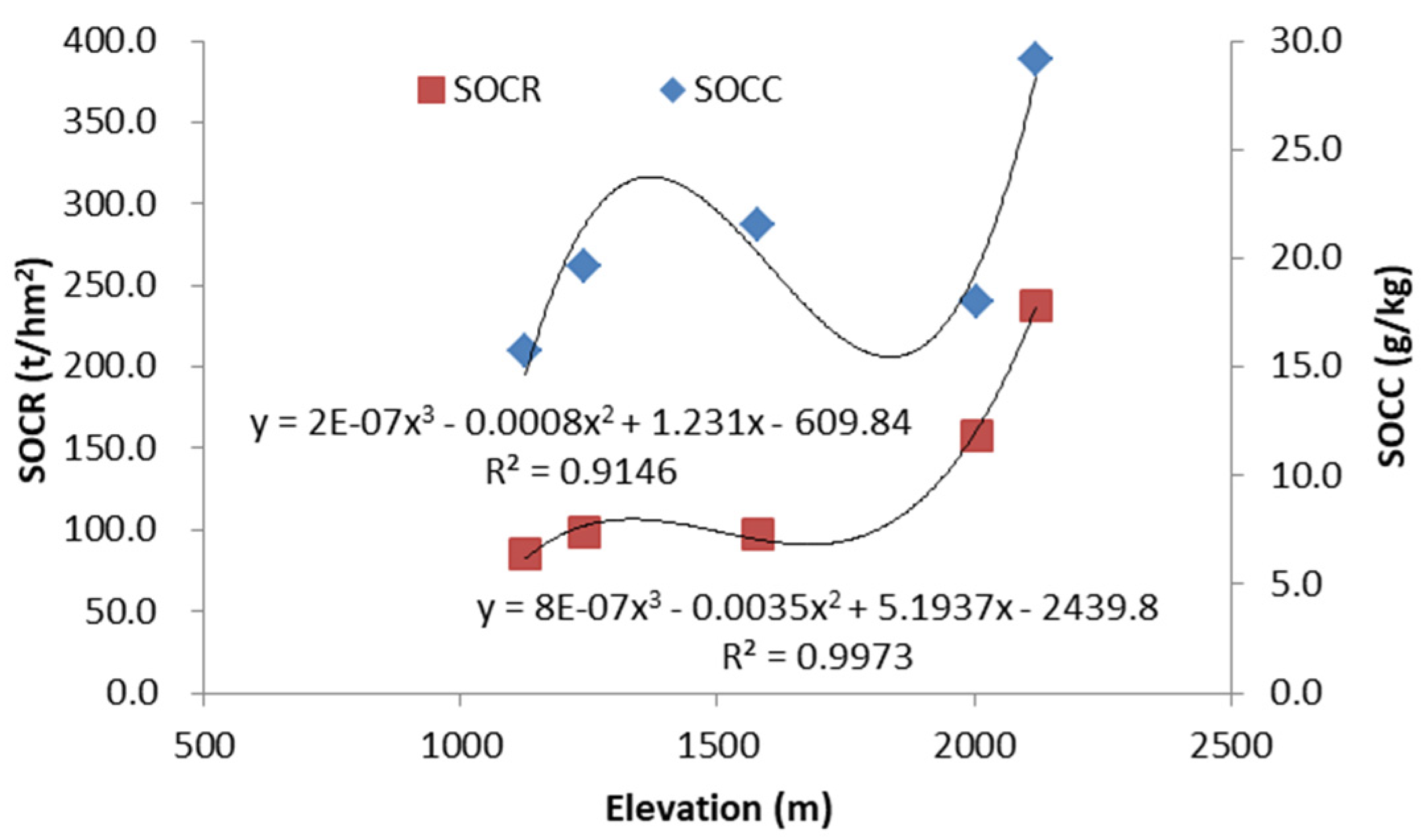
3.1.2. Vertical Distribution of SOC

Table 3. Mean, coefficients of variation (CV), and standard deviation (SD) of soil organic carbon concentrations (SOCCs) in the different soil layers. The soil layer was divided into 0–15 cm, 15–30 cm, 30–45 cm, 45–60 cm, and >60 cm. Same lowercase letters indicate no significant difference between soil layers in the same forest community (p > 0.05). Numbers in parentheses are standard errors.

Forest Communities	Statistical Parameters	Soil Layers
		0–15 cm	15–30 cm	30–45 cm	45–60 cm
PEF	Mean (g/kg)	39.37 (2.67) a	24.16 (3.53) b	12.17 (1.48) c	13.45 (3.67) c
	SD	8.61	4.51	0.39	0.71
	CV	0.219	0.187	0.032	0.052
CLF	Mean (g/kg)	28.93 (4.31) a	11.004 (2.25) b	7.47 (0.20) b	7.01 (0.35) b
	SD	8.61	4.51	0.39	0.71
	CV	0.30	0.41	0.05	0.10
SSF	Mean (g/kg)	31.25 (3.91) a	12.86 (3.20) b	9.23 (3.24) b	6.90 (1.48) b
	SD	6.77	5.55	5.61	2.57
	CV	0.22	0.43	0.61	0.37
CSF	Mean (g/kg)	25.35 (5.81) a	25.15 (4.81) a	26.74 (1.56) a	28.469 (3.33) a
	SD	10.06	8.34	2.70	9.23
	CV	0.40	0.33	0.10	0.32
SF	Mean (g/kg)	44.42 (6.72) a	19.67 (2.33) b	10.80 (1.88) bc	8.40 (1.33) c
	SD	15.03	5.20	4.21	2.98
	CV	0.34	0.27	0.39	0.36
FLF	Mean (g/kg)	36.39 (5.72) a	20.36 (1.72) b	5.88 (1.65) c	4.89 (2.65) c
	SD	8.08	2.44	2.34	3.74
	CV	0.22	0.12	0.40	0.77
PMF	Mean (g/kg)	12.45	6.51	3.20	1.17
Total	Mean (g/kg)	32.90 (2.72) a	17.51 (1.63) b	11.32 (1.55) c	10.60 (1.86) c
	SD	12.74	7.62	7.28	8.71
	CV	0.38	0.44	0.64	0.82

PMF refers to only one repetition, without ANOVA and Multiple Comparisons.

shows that the SOC distribution exhibited obvious vertical gradient changes and generally decreased with the increase in soil depth. The average SOCC in the 0–15 cm soil layer was 32.896 g/kg, while that in the >60 cm soil layer was only 3.664 g/kg. The gradient variation of the SOCC in the different forest communities was different. The SOCC in the 0–15 cm soil layer in the SF was the highest, and it was the lowest in the 45–60 cm soil layer in PMF. The SOCC of all the forest communities decreased by 5.43 g/kg with every 10 cm increase in soil depth. The CV of SOCC increased with the increase in soil depth. The CV in the 0–15 cm soil layer was the smallest (0.387), and the CV in the 45–60 cm soil layer was the largest (0.821). However, the CV decreased when the soil layer was larger than 60 cm.

The results of the ANOVA using SPSS 23.0 (Statistical Product and Service Solutions, IBM, USA) show that there were significant differences in the SOCC among different soil layers (p = 0.000 < 0.01). The multiple comparisons show that there were significant differences between the 0–15 cm soil layer and the 15–30 cm, 30–45 cm, 45–60 cm, and >60 cm soil layers, and between the 15–30 cm soil layer and the 30–45 cm, 45–60 cm, and >60 cm soil layers (p < 0.05). The results show that the SOC distributions in the Maoershan Mountains had obvious surface aggregation, and the roots of the trees had a great influence on the SOC distributions.

According to Figure 4, the distribution of FSOC also increases with the increase in elevation, in which the SOCC and SOCR increase by 1.80 g/kg and 18.23 t/hm² with every 100 m increase in elevation, respectively.

3.2. RDA of SOC and Environmental Factors

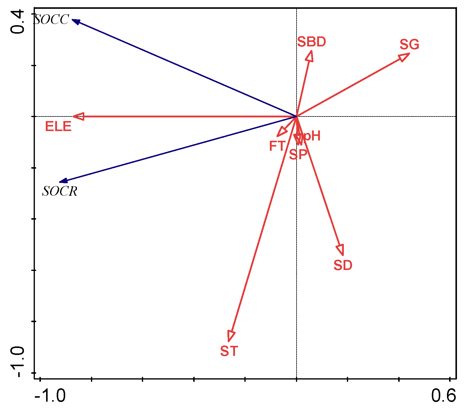
3.2.1. Interpretation of RDA Results

According to the RDA results (

Table 4. Redundancy analysis (RDA) between soil organic carbon (SOC) and environmental factors.

Axis	1	2	3	4
Eigenvalues	0.82	0.10	0.09	0.00
Explained variation (cumulative)	81.56	91.37	99.94	100
Pseudo-canonical correlation	0.95	1.00	0	0
Explained fitted variation (cumulative)	89.27	100

), the relationship between SOC and the first ranking axis was the largest (r = 0.95), which could explain 89.27% of the relationship between SOC and environmental factors. The correlation coefficient between SOC and the second ranking axis was 1.00, and the two ranking axes could explain 100% of the relationship between SOC and environmental factors. The eigenvalues of the first and second axes accounted for 91.37% of the total eigenvalues, indicating that the ranking effect was very good and could better express the influence of environmental factors on the spatial variation in SOC. Pearson’s test showed that pseudo-F = 6.6, p = 0.01 < 0.01, indicating that there was a strong correlation between SOC and environmental factors, and the difference in SOC caused by environmental factors had statistical and ecological significance.

Since the total variance explained by RDA1 and RDA2 is very high, there is a possibility of collinearity among explanatory variables. SPSS 23.0 was used for the collinearity diagnosis. The results show that the eigenvalue of explanatory variables with more than six dimensions was about 0, and the condition index of more than four dimensions was more than 10 (

Table 5. Eigenvalue, condition index, and variance ratio of collinearity diagnosis of explanatory variables.

Model	Eigenvalue	Condition Index	Variance Ratio
			Constant	FT	ELE	SP	SG	ST	pH	SBD	SD
1	8.44	1.00	0.00	0.00	0.00	0.00	0.00	0.00	0.00	0.00	0.00
2	0.29	5.44	0.00	0.08	0.01	0.06	0.00	0.00	0.00	0.00	0.00
3	0.13	7.95	0.00	0.02	0.02	0.01	0.01	0.04	0.00	0.00	0.00
4	0.08	10.07	0.00	0.00	0.11	0.06	0.00	0.08	0.00	0.00	0.00
5	0.05	12.43	0.00	0.41	0.11	0.17	0.00	0.02	0.00	0.00	0.00
6	0.00	44.78	0.01	0.03	0.04	0.47	0.65	0.14	0.01	0.02	0.06
7	0.00	58.34	0.28	0.03	0.02	0.04	0.00	0.11	0.01	0.35	0.00
8	0.00	101.32	0.48	0.36	0.52	0.00	0.32	0.41	0.03	0.62	0.46
9	0.00	129.55	0.23	0.07	0.16	0.18	0.02	0.20	0.95	0.00	0.47

), which proves that there might be collinearity among the explanatory variables. However, no two factors with correlation coefficients close to one were found in the correlation coefficient matrix of the explanatory variables. The largest correlation coefficients were pH and SD, which were 0.658. This indicates that collinearity among explanatory variables had little influence on the response variables.

3.2.2. RDA Ranking of SOC and Environmental Factors

Through the RDA of SOC and environmental factors, we determined the environmental factors that were significantly related to SOC (Figure 5). In the RDA sequencing diagram, the length of the arrow line represents the degree of correlation between a certain environmental factor and the SOCC and SOCR. The longer the line is, the greater the correlation; the shorter the line is, the smaller the correlation. The included angle between the arrow line and the ranking axis represents the correlation between a certain environmental factor and the ranking axis. The smaller the included angle, the greater the correlation is; the larger the included angle, the smaller the correlation is.

According to Figure 5, RDA1 and RDA2 together explained 91.37% of the variance, and there was a strong correlation between SOC and environmental factors. The SOCC and SOCR were positively correlated with ELE, ST, and FT and negatively correlated with SP, pH, SG, and SBD. The SOCC and SOCR had the strongest positive correlation with ELE, the SOCC had the strongest negative correlation with SG, and the SOCR had the strongest negative correlation with SP and pH. In other words, the SOCC and SOCR showed an obvious increasing trend with the increase in ELE, the SOCC decreased significantly with the increase in SG, and the SOCR decreased significantly with the increase in SP and pH.

Table 6. Explanation rate and significance testing of environmental factors.

Environmental Factor	Explanation Rate (%)	Contribution Rate (%)	Pseudo-F	p
ELE	61.90	67.80	19.50	0.00
FT	11.10	12.20	4.50	0.04
ST	9.30	10.20	5.30	0.02
SBD	4.60	5.00	3.20	0.09
SP	2.40	2.60	1.80	0.19
SD	1.60	1.80	1.30	0.28
pH	0.30	0.30	0.20	0.68
SG	<0.10	<0.10	<0.10	0.85

shows that the effect of environmental factors on the spatial variation in SOC was ELE > FT > ST > SBD > SP > SD > SG > pH. Among these factors, ELE contributed the most to the spatial variation in SOC (67.80 %), followed by FT and ST (12.20 % and 10.20 %).

3.3. Quantitative Separation and Interpretation Ability of Environmental Factors

The environmental factors affecting the SOCC and SOCR were divided into three categories: forest factors, topographic factors, and soil factors. Forest factors included FT and SD; topographic factors included ELE, SP, and SG; and soil factors included ST, pH, and SBD. The overall interpretation ability of environmental factors regarding the variation in the SOCC and SOCR was 91.40%, and the unexplained portion amounted to only 8.60%. In other words, environmental factors caused 91.40% of the variation in SOC. The three categories of the environmental factors and SOCC and SOCR were, respectively, subjected to RAD to obtain the quantitative separation results of the impact of environmental factors on SOC. Topographic factors alone caused 66.10% of the variation in SOC, soil factors alone caused 16.5% of the variation, and forest factors alone caused 9.00% of the variation. The interactions between environmental factors partially offset each other, reducing the variation in SOC.

According to the results of the pseudo-canonical testing listed in

Table 7. Pseudo-canonical testing results of soil organic carbon (SOC) variation caused by environmental factors.

Environmental Factors	Pseudo-F	p
Forests	0.50	0.66
Topographic	6.50	0.00
Soil	0.70	0.06
All environmental factors	6.60	0.01

, pseudo-F_topographic = 6.5; p_topographic = 0.00 < 0.01. These results indicate that the variation in SOC caused by topographic factors had statistical and ecological significance, and the explanation rate of topographic factors regarding the spatial distribution difference in SOC was relatively higher; moreover, ELE was the most important factor. In addition, the results of the pseudo-canonical testing showed pseudo-F_soil = 0.7, p_soil = 0.64 > 0.05, and pseudo-F_forests = 0.5, p_forest = 0.66 > 0.05, indicating that the hypothesis of SOC variation being caused only by soil factors or forest factors was not valid.

4. Discussion

4.1. Response of SOC Distribution to Forest Community

The main forest communities in the Maoershan Mountains include PEF, CLF, SSF, CSF, SF, FLF, and PMF, among which CSF, SSF, FLF, PMF, and SF were natural forests, while CLF and PEF were plantations. In general, the SOCC of natural forests was higher than that of plantations, and the degree of variation in SOC in space was higher after multiple cutting and the utilization of plantation. Moreover, the distribution of FSOC increased with elevation, which was consistent with the regular distribution of natural forests along elevation [35], indicating that elevation had only an indirect effect on SOC. The conclusion that the distribution of SOC changes with elevation is consistent with the conclusion of Cao Xinguang et al.’s study on the distribution characteristics of SOC at different elevations in Northern subtropical regions with the Guifeng Mountains of Eastern Hubei as an example [41]. That is different from Huang Bin et al.’s study on the characteristics of SOC and its components’ altitudinal gradient in Nanling Mountains, which concluded that “soil organic carbon increases first and then decreases with the increase of elevation” [42]. The conclusion that elevation has only an indirect effect on SOC is similar to that of Shen Kaihui et al. [43].

The SOCC of CSF was the highest, and that of PMF was the lowest. Duan et al. believe that CSF is the only well-preserved primary forest, and this area is the flattest region. The PMF is a typical secondary forest, formed after the degradation of the primary forest. It is located in a region with poor site environmental conditions, a thin soil layer, and a large slope [35]. Although the hypothesis that forest factors (forest community type, forest density) alone cause the variation in SOC is not verified, the spatial heterogeneity of SOC distribution is extremely strongly correlated with the variation in the forest community. This conclusion was similar to the study of Deng Xiaojun et al. [44,45]. The effect of the forest community on SOC distribution was related to forest litter, which has been verified by many studies. Raich et al.’s research concluded that forest litters have a great influence on SOC distribution [46,47,48]. Forest litter was the main source of SOC and offered an important surface protection layer. It affected the distribution of SOC by changing the precipitation leaching process and SOC migration path, which is the fundamental reason for the difference in SOC distribution in different forest communities [10,49]. The change in forest litter is directly affected by stand factors [50]. The study on the effects of forest litter on SOC distribution is important to reveal the response of SOC to forest community succession, which requires more attention in future studies.

4.2. Response of SOC Distribution to Elevation Gradient

In the Maoershan Mountains, the differences in SOCC were not only driven by the forest community type, but also by the elevation and soil layer position. In general, the SOC distribution increased with the rise in elevation, and the SOCC increased by 1.02 g/kg with every 100 m increase in elevation, while the SOCR increased by 10.40 g. In this study, SF appeared at multiple elevations, and SOCC had an obvious trend of increasing gradually with the elevation (Figure 6). At the same time, the spatial variation in SOCC was great due to the influence of meteorological factors at different elevations. The SOC distribution in the Maoershan Mountains showed an increasing trend with rising elevation, which is similar to the results of Gong Li et al. [51]. According to Qin Hailong et al., the SOCC of each soil layer in the Maoershan Mountains increased with the increase in elevation and was the largest at 2100 m [52]. The main reason why the distribution of SOC increases with the rising elevation is that, with the rise in elevation, the temperature decreases, the decomposition of organic matter slows down, and plant litter increases, so the SOCC is high. However, in low-elevation areas, due to the sufficient amount of heat, the conditions are conducive to the growth of vegetation and the accumulation of plant organic carbon. At the same time, due to the high temperatures, the decomposition rate of litter becomes faster, and the accumulation of SOC decreases. SOC in different soil layers showed different responses to elevation, and the upper soil was more sensitive to changes in elevation [17]. Elevation is an important indirect factor affecting the distribution of FSOC, which affects the distribution of the forest, the growth of forest vegetation, and soil biological activities.

4.3. Response of SOC Distribution to Soil Depth

In the Maoershan Mountains, the contribution of soil factors to the variation in FSOC is small, but the distribution of FSOC decreases significantly with the increase in soil depth. With the increase in soil depth, the SOCC of all forest communities showed a decreasing trend [52]. The SOCC in the 0–15 cm forest soil layer in the Maoershan Mountains was the highest, which was significantly different from other soil layers, and the distribution of FSOC displayed obvious surface aggregation. However, due to the different study areas and soil types, the depth of SOC surface aggregation was different. Some researchers believe that SOC surface aggregation occurs in the 0–40 cm soil layer [17], while others believe that it occurs in the 0–20 cm soil layer [44,53], and some even believe that it occurs in the 0–10 cm soil layer [54]. We concluded that the surface aggregation of FSOC in the Maoershan Mountains occurred in the 0–15 cm soil layer, and the variation in the SOCC in the 0–15 cm soil layer was the smallest, while the variation in the 45–60 cm soil layer was the largest. This conclusion is similar to that obtained in the study of Pang Shengjiang in the Maoershan Mountains. The SOCC values of the topsoil in sempervirent broadleaved forests, sempervirent deciduous broadleaved forests, coniferous and broadleaved mixed forests, and shrub forests were 151.31 g/kg, 145.33 g/kg, 90.61 g/kg, and 86.92 g/kg, respectively [55].

4.4. Response of SOC Distribution to the Interactions between Environmental Factors

FSOC has a good regulatory effect on soil physical, chemical, and biological characteristics, and its distribution is influenced by forest and other environmental factors, as well as climate change [24,28]. There was a strong correlation between FSOC and environmental factors in the Maoershan Mountains, among which SOC had the strongest positive correlation with elevation and the strongest negative correlation with SG. Elevation and soil layer thickness had significant effects on the spatial distribution of SOC, and they were important environmental factors affecting the changes in the SOCC and SOCR in the Maoershan Mountains. Our conclusion is consistent with the study of Wu Xiaogang [17]. Although forest factors caused only 9.0% of the variation in FSOC, forest plants are their main source and play a decisive role in the spatial distribution of FSOC because FSOC is the carbon element in humus, plant, and animal residues, as well as the microbial bodies formed by microorganisms [56]. The influence process and mechanism of forest plants regarding the spatial distribution of SOC are complex and often occur through environmental factors. In particular, soil animal activities and soil microenvironment changes cause changes in soil carbon pools [18]. In addition, disturbances caused by human activities affect SOC emissions and have a great effect on global ecological environmental change [57].

RDA is a useful method with which to analyze and explain the internal relationship between the spatial variation in SOC and environmental factors, but its analysis obscures the decisive role of forest plants themselves and does not consider human activities with specific quantitative indicators. Therefore, when studying the relationship between the spatial distribution of FSOC and environmental factors in the future, it is necessary to pay more attention to the forest itself, to soil enzymes and microbial activities, and to the influence of human disturbances. It is also necessary to select more scientific and reasonable methods by which to conduct the study.

5. Conclusions

Forest soil organic carbon (FSOC) distribution and its response to environmental factors are the most important scientific and technological requirements for the scientific and effective management of the forest soil carbon pool, the evaluation of carbon sink function and economic effects, and the implementation of the “carbon peak and carbon neutrality” strategy. Our study on the interaction between SOC distribution and environmental factors shows that the SOC distribution was the result of the combined action of many environmental factors. The SOC distribution was sensitive to elevation, slope, forest community types, and soil layer thickness, and the SOC distribution had obvious surface aggregation characteristics. SOC distribution was greater in high-elevation areas, and that in natural forests was greater than that in plantations, and the spatial variation in SOC distribution in plantations was higher due to the effect of cutting and utilization. Secondary forests formed after degradation have low vegetation cover, poor growth, and a low SOCC due to poor environmental conditions at the site. The conversion of plantations to natural forests will increase SOC, and excessive interference with forests will aggravate SOC emissions. Therefore, in order to support the realization of the regional “carbon peak and carbon neutrality” goal, it is necessary to strengthen the protection of natural forests and the restoration of secondary forests in the Maoershan Mountains, especially the protection of natural forests in high-elevation areas, the scientific and rational management of plantations, the limitation of human interference in forests on steep slopes, and the reduction in CO₂ emissions in forest soil in order to constantly improve the function of the forest soil carbon pool.

References

1. Akram, M.A.; Wang, X.; Hu, W.; Xiong, J.; Zhang, Y.; Deng, Y.; Ran, J.; Deng, J. Convergent Variations in the Leaf Traits of Desert Plants. Plants 2020, 9, 990. [Google Scholar] [CrossRef] [PubMed]
2. Li, H.; Wu, Y.; Chen, J.; Zhao, F.; Wang, F.; Sun, Y.; Zhang, G.; Qiu, L. Responses of soil organic carbon to climate change in the Qilian Mountains and its future projection. J. Hydrol. 2021, 596, 126110. [Google Scholar] [CrossRef]
3. Cardon, Z.G.; Hungate, B.A.; Cambardella, C.A.; Chapin, F.S.; Field, C.B.; Holland, E.A.; Mooney, H.A. Contrasting effects of elevated CO2 on old and new soil carbon pools. Soil Biol. Biochem. 2001, 33, 365–373. [Google Scholar] [CrossRef]
4. Osipov, A.F.; Bobkova, K.S.; Dymov, A.A. Carbon stocks of soils under forest in the Komi Republic of Russia. Geoderma Reg. 2021, 27, e00427. [Google Scholar] [CrossRef]
5. Angst, G.; Mueller, K.E.; Nierop, K.G.J.; Simpson, M.J. Plant- or microbial-derived? A review on the molecular composition of stabilized soil organic matter. Soil Biol. Biochem. 2021, 156, 108189. [Google Scholar] [CrossRef]
6. Wiesmeier, M.; Urbanski, L.; Hobley, E.; Lang, B.; von Lützow, M.; Marin-Spiotta, E.; van Wesemael, B.; Rabot, E.; Ließ, M.; Garcia-Franco, N.; et al. Soil organic carbon storage as a key function of soils–A review of drivers and indicators at various scales. Geoderma 2019, 333, 149–162. [Google Scholar] [CrossRef]
7. Li, Q.; Huang, Y.; Liu, G.; Zeng, X. The Contents and Character Of Heavy Metals Of Main Soil Types In Three Gorge Reservoir. Acta Pedol. Sin. 2004, 41, 301–304. [Google Scholar]
8. Pan, Y.; Birdsey, R.A.; Fang, J.; Houghton, R.; Kauppi, P.E.; Kurz, W.A.; Phillips, O.L.; Shvidenko, A.; Lewis, S.L.; Canadell, J.G.; et al. A large and persistent carbon sink in the world’s forests. Science 2011, 333, 988–993. [Google Scholar] [CrossRef]
9. IPCC Climate Change. The physical science basis. Contrib. Work. Group I Fifth Assess. Rep. Intergov. Panel Clim. Change 2013, 1535, 2013. [Google Scholar]
10. Houghton, R.A. Land-use change and the carbon cycle. Glob. Chang. Biol. 1995, 1, 275–287. [Google Scholar] [CrossRef]
11. Zhou, G.; Liu, S.; Li, Z.; Zhang, D.; Tang, X.; Zhou, C.; Yan, J.; Mo, J. Old-growth forests can accumulate carbon in soils. Science 2006, 314, 1417. [Google Scholar] [CrossRef] [PubMed]
12. Schrumpf, M.; Schulze, E.D.; Kaiser, K.; Schumacher, J. How accurately can soil organic carbon stocks and stock changes be quantified by soil inventories? Biogeosciences 2011, 8, 1193–1212. [Google Scholar] [CrossRef]
13. Ter Braak, C.J.; Smilauer, P. CANOCO Reference Manual and CanoDraw for Windows User’s Guide: Software for Canonical Community Ordination, version 4.5; 2002. Available online: https://www.scienceopen.com/document?vid=f1f55dd4-0d25-4b5f-ba80-1b47296bc070 (accessed on 18 April 2023).
14. Smith, P.; House, J.I.; Bustamante, M.; Sobocka, J.; Harper, R.; Pan, G.; West, P.C.; Clark, J.M.; Adhya, T.; Rumpel, C.; et al. Global change pressures on soils from land use and management. Glob. Change Biol. 2016, 22, 1008–1028. [Google Scholar] [CrossRef] [PubMed]
15. Hou, G.; Delang, C.O.; Lu, X.; Gao, L. A meta-analysis of changes in soil organic carbon stocks after afforestation with deciduous broadleaved, sempervirent broadleaved, and conifer tree species. Ann. For. Sci. 2020, 77, 92. [Google Scholar] [CrossRef]
16. Pita, G.; Gielen, B.; Zona, D.; Rodrigues, A.; Rambal, S.; Janssens, I.A.; Ceulemans, R. Carbon and water vapor fluxes over four forests in two contrasting climatic zones. Agric. For. Meteorol. 2013, 180, 211–224. [Google Scholar] [CrossRef]
17. Wu, X.; Wang, W.; Li, B.; Liang, Y.; Liu, Y. Altitudinal Gradient of Soil Organic Carbon in Forest Soils in the Mid-Subtropical Zone of China. Acta Pedol. Sin. 2020, 57, 1539–1547. [Google Scholar]
18. Li, G.; Shi, L.; Zhang, Z.; Grace, J.; Yang, M.; Wu, S.; Lei, G. Distribution of soil organic carbon and potential carbon sequestration in an alpine meadow grazed by domesticated yak in Zeku, Qinghai-Tibetan Plateau, China. Carbon Manag. 2019, 10, 135–147. [Google Scholar] [CrossRef]
19. Khosravi Aqdam, K.; Yaghmaeian Mahabadi, N.; Ramezanpour, H.; Rezapour, S.; Mosleh, Z.; Zare, E. Comparison of the uncertainty of soil organic carbon stocks in different land uses. J. Arid Environ. 2022, 205, 104805. [Google Scholar] [CrossRef]
20. Breg Valjavec, M.; Čarni, A.; Žlindra, D.; Zorn, M.; Marinšek, A. Soil organic carbon stock capacity in karst dolines under different land uses. Catena 2022, 218, 106548. [Google Scholar] [CrossRef]
21. Grandy, A.S.; Robertson, G.P. Land-Use Intensity Effects on Soil Organic Carbon Accumulation Rates and Mechanisms. Ecosystems 2007, 10, 59–74. [Google Scholar] [CrossRef]
22. Ahirwal, J.; Gogoi, A.; Sahoo, U.K. Stability of soil organic carbon pools affected by land use and land cover changes in forests of eastern Himalayan region, India. Catena 2022, 21, 106308. [Google Scholar] [CrossRef]
23. Jobbagy, E.G.; Jackson, R.B. The Vertical Distribution of Soil Organic Carbon and Its Relation to Climate and Vegetation. Ecol. Appl. 2000, 10, 423–436. [Google Scholar] [CrossRef]
24. Du, X.; Wang, H. Active Components of Forest Soil Organic Carbon and Its Influencing Factors in China. World For. Res. 2022, 35, 76–81. [Google Scholar] [CrossRef]
25. Woodwell, G.M.; Whittaker, R.H.; Reiners, W.A.; Likens, G.E.; Delwiche, C.C.; Botkin, D.B. The biota and the world carbon budget. Science 1978, 199, 141–146. [Google Scholar] [CrossRef]
26. Dixon, R.K.; Solomon, A.M.; Brown, S.; Houghton, R.A.; Trexier, M.C.; Wisniewski, J. Carbon pools and flux of global forest ecosystems. Science 1994, 263, 185–190. [Google Scholar] [CrossRef] [PubMed]
27. Bradshaw, C.J.A.; Warkentin, I.G. Global estimates of boreal forest carbon stocks and flux. Glob. Planet. Change 2015, 128, 24–30. [Google Scholar] [CrossRef]
28. Wei, H.; Ma, X.; Liu, A.; Feng, L.; Huang, Y. Review on carbon cycle of forest ecosystem. Chin. J. Eco-Agric. 2007, 15, 188–192. [Google Scholar]
29. Liu, S.; Wang, H.; Luan, J. A review of research progress and future prospective of forest soil carbon stock and soil carbon process in China. Acta Ecol. Sin. 2011, 31, 5437–5448. [Google Scholar]
30. Zhang, Y.-R.; Ouyang, X.; Chu, G.-W.; Zhang, Q.-M.; Liu, S.-Z.; Zhang, D.-Q.; Li, Y.-L. Spatial heterogeneity of soil organic carbon and total nitrogen in a monsoon evergreen broadleaf forest in Dinghushan, Guangdong, China. Chin. J. Appl. Ecol. 2014, 25, 19–23. [Google Scholar] [CrossRef]
31. Wang, J.; Li, H.; Duan, W.; Tang, D.; Wang, S.; Liu, X.; Huang, H. Runoff Processes and the Influencing Factors in a Small Forested Watershed of Upper Reaches of Lijiang River. Sci. Silvae Sin. 2013, 49, 149–153. [Google Scholar]
32. Huang, Y.; Chen, G.; Liu, B.; Lin, S.; Yang, X. Formation Characteristics and Taxonomy of Soils in Maoer Mountains in Guangxi. Chin. Agric. Sci. Bull. 2010, 26, 188–193. [Google Scholar]
33. Huang, J.; Jiang, D. Comprehensive and Scientific Investigation in Guangxi Maoershan Nature Reserve; Hunan Science and Technology Press: Changsha, China, 2002. [Google Scholar]
34. Wang, H.; Yan, W.; Wang, J.; Duan, W. Exploring Distribution Rules and Variation Trends of Precipitation in the Upper Lijiang River from 1951 to 2016, Guangxi Province, China. J. Coast. Res. 2020, 105, 1–5. [Google Scholar] [CrossRef]
35. Duan, W.; Wang, J. Vertical distribution pattern and determinant analysis of forest community in Maoer Mountain National Nature Reserve. Ecol. Environ. Sci. 2013, 22, 563–566. [Google Scholar] [CrossRef]
36. Webster, R. Quantitative Spatial Analysis of Soil in the Field. In Soil Restoration, Advances in Soil Science; Springer: New York, NY, USA, 1985; Volume 3, pp. 1–70. [Google Scholar]
37. Trangmar, B.B.; Yost, R.S.; Uehara, G. Application of Geostatistics to Spatial Studies of Soil Properties. Adv. Agron. 1986, 38, 45–94. [Google Scholar] [CrossRef]
38. GB/T 33027-2016; Institute of Forest Ecology, Environment and Protection, Chinese Academy of Forestry, Method for Long-Term Positioning and Observation of Forest Ecosystems. In General Administration of Quality Supervision, Inspection and Quarantine of the People’s Republic of China; Standardization Administration of China: Beijing, China, 2016; p. 112.
39. Haluschak, P. Laboratory methods of soil analysis. Can.-Manit. Soil Surv. 2006, 3–133. [Google Scholar]
40. Nelson, D.W.; Sommers, L.E. Total carbon, organic carbon, and organic matter. Methods Soil Anal. Part 3 Chem. Methods 1996, 5, 961–1010. [Google Scholar]
41. Cao, X.G.; Yue, W.P.; Deng, J. Soil organic carbon distribution characteristics along an altitudinal gradient in the north-ern subtropical region:a case study in Guifeng Mountains of Eastern Hubei, China. J. Guangxi Norm. Univ. 2021, 39, 174–182. [Google Scholar] [CrossRef]
42. Huang, B.; Wang, Q.-Q.; Li, D.-Q.; Xiao, H.-B.; Nie, X.-D.; Yuan, Z.-J.; Zheng, M.-G.; Liao, Y.S.; Liang, C. Variation Characteristics of Organic Carbon and Fractions in Soils along the Altitude Gra-dient in Nanling Mountains. Chin. J. Soil Sci. 2022, 53, 374–383. [Google Scholar] [CrossRef]
43. Shen, K.-H.; Wei, S.-G.; Li, L.; Chu, X.-X.; Zhong, J.-J.; Zhou, J.-G.; Zhao, Y. Spatial Distribution Patterns of Soil Organic Carbon in Karst Forests of the Lijiang River Basin and Its Driving Factors. Environ. Sci. 2022, 216, 106409. [Google Scholar] [CrossRef]
44. Zhang, Z.; Huang, X.; Zhou, Y. Spatial heterogeneity of soil organic carbon in a karst region under different land use patterns. Ecosphere 2020, 11, e03077. [Google Scholar] [CrossRef]
45. Deng, X.; Zhu, L.; Song, X.-c.; Tang, J.; Tan, Y.-b.; Deng, N.-n.; Zheng, W.; Cao, J. Soil Ecological Stoichiometry Characteristics of Different Stand Types in Maoershan Nature Reserve. Chin. J. Soil Sci. 2022, 53, 366–373. [Google Scholar] [CrossRef]
46. Raich, J.W.; Schlesinger, W.H. The global carbon dioxide flux in soil respiration and its relationship to vegetation and climate. Tellus B 1992, 44, 81–99. [Google Scholar] [CrossRef]
47. Vesterdal, L.; Clarke, N.; Sigurdsson, B.D.; Gundersen, P. Do tree species influence soil carbon stocks in temperate and boreal forests? For. Ecol. Manag. 2013, 309, 4–18. [Google Scholar] [CrossRef]
48. Don, A.; Schumacher, J.; Freibauer, A. Impact of tropical land-use change on soil organic carbon stocks—A meta-analysis. Glob. Change Biol. 2011, 17, 1658–1670. [Google Scholar] [CrossRef]
49. Hong, X.; Li, M.; Yu, T.-w.; Yan, Q.; Wei, Q.; Hu, Y.-l. Effects of aboveground and belowground litter inputs on the balance of soil new and old organic carbon under the typical forests in subtropical region. Chin. J. Appl. Ecol. 2021, 32, 825–835. [Google Scholar] [CrossRef]
50. Yu, X.; Xu, C.; Zhu, Y.; Xu, X. Litterfall production and its relation to stand structural factors in a subtropical evergreen broadleaf forest. J. Zhejiang AF Univ. 2016, 33, 991–999. [Google Scholar]
51. Gong, L.; Liu, G.; Li, Z.; Ye, X.; Wang, H. Altitudinal changes in nitrogen, organic carbon, and its labile fractions in different soil layers in an Abies faxoniana forest in Wolong. Acta Ecol. Sin. 2017, 37, 4696–4705. [Google Scholar]
52. Qin, H.; Fu, X.; Lu, Y.; Wei, X.; Li, B.; Jia, C. Soil C: N: P stoichiometry at different altitudes in Mao’er Mountain, Guangxi, China. Chin. J. Appl. Ecol. 2019, 30, 711–717. [Google Scholar] [CrossRef]
53. Liu, K.; Li, M.; Li, L.; Tian, K.; Wang, Z.; Qu, M.; Fan, Y.N.; Huang, B. Spatial heterogeneity of the soil organic carbon density and its driving factors in the water source area of the Middle Route of China South-to-North Water Diversion Project. J. Nanjing For. Univ. 2022, 46, 35–43. [Google Scholar]
54. Zhao, Q.; Liu, S.; Chen, K.; Wang, S.; Wu, C.; Li, J.; Lin, Y. Change characteristics and influencing factors of soil organic carbon in Castanopsis eyrei natural forests at different altitudes in Wuyishan Nature Reserve. Acta Ecol. Sin. 2021, 41, 5328–5339. [Google Scholar]
55. Pang, S.; Zhang, P.; Yang, B.; Jia, H.; Huang, B.; Liu, S. The distribution of organic carbon and soil nutrients under four forest types in karst mountain areas of northwest Guangxi, China. J. Cent. South Univ. For. Technol. 2018, 38, 60–64+71. [Google Scholar] [CrossRef]
56. Liu, M.; Sun, J.; Xu, X. Imbalance of soil elements drives the degradation of alpine grasslands. Chin. J. Ecol. 2020, 39, 2574–2580. [Google Scholar] [CrossRef]
57. Fang, J.; Yu, G.; Liu, L.; Hu, S.; Chapin, F.S., 3rd. Climate change, human impacts, and carbon sequestration in China. Proc. Natl. Acad. Sci. USA 2018, 115, 4015–4020. [Google Scholar] [CrossRef] [PubMed]
Figure 1. The location of the Maoershan Mountains, Guilin, Guangxi Province of China. The research site is located in the Maoershan Mountains.
Sustainability 15 08716 g001
Figure 2. Soil organic carbon concentrations (SOCCs) with red rectangle and soil organic carbon reserve (SOCR) with blue line of different forest communities in the Maoershan Mountains. The forest community includes Phyllostachys edulis forests (PEF), Cunninghamia lanceolata forests (CLF), Schima superba forests (SSF), Cyclobalanopsis stewardiana forests (CSF), shrub forests (SF), Fagus longipetiolata forests (FLF), and Pinus Massoniana forests (PMF). Same lowercase letters indicate no significant difference between forest communities (p > 0.05). Letters a, b, c and d represent significant differences in individual parameters among the different stands by Tukey’s HSD post hoc tests (p < 0.05).
Sustainability 15 08716 g002
Figure 3. Coefficient of variation (CV) with bule line and average value of soil organic carbon concentrations (SOCC) with red line in different forest communities in the Maoershan Mountains.
Sustainability 15 08716 g003
Figure 4. Variation in trend of soil organic carbon concentrations (SOCCs) and soil organic carbon reserve (SOCR) of different forest communities with elevation in the Maoershan Mountains.
Sustainability 15 08716 g004
Figure 5. RDA analysis of the relationship between soil organic carbon (SOC) and environmental factors in the Maoershan Mountains. The environmental factors include elevation (ELE), slope gradient (SG), slope position (SP), stand density (SD), soil thickness (ST), soil pH (pH), soil bulk density (SBD), and forest community type (FT).
Sustainability 15 08716 g005
Figure 6. Variation in trend of soil organic carbon concentrations (SOCCs) and soil organic carbon reserve (SOCR) with the rise of elevation (1100–2200 m) in shrub forests (SF) of the Maoershan Mountains.
Sustainability 15 08716 g006