The Multi-Scale Model Method for U-Ribs Temperature-Induced Stress Analysis in Long-Span Cable-Stayed Bridges through Monitoring Data

Abstract

Temperature is one of the important factors that affect the fatigue failure of the welds in orthotropic steel desks (OSD) between U-ribs and bridge decks. In this study, a new analysis method for temperature-induced stress in U-ribs is proposed based on multi-scale finite element (FE) models and monitoring data First, the long-term temperature data of a long-span cable-stayed bridge is processed. This research reveals that a vertical temperature gradient is observed rather than a transverse temperature gradient on the long-span steel box girder bridge with tuyere components. There is a linear relationship between temperature and temperature-induced displacement, taking into account the time delay effect (approximately one hour). Then, a multi-scale FE model is established using the substructure method to condense each segment of the steel girder into a super-element, and the overall bridge temperature-induced displacement and temperature-induced stress of the local U-rib on the OSD are analyzed. The agreement between the calculated temperature-induced stresses and measured values demonstrates the effectiveness of the multi-scale modeling strategy. This approach provides a valuable reference for the evaluation and management of bridge safety. Finally, based on the multi-scale FE model, the temperature-induced strain distribution of components on the OSD is studied. This research reveals that the deflection of the girder continually changes with the temperature variation, and the temperature-induced strain of the girder exhibits a variation range of approximately 100 με.

1. Introduction

Orthotropic steel desks (OSD) are widely used in long-span steel box girder bridges due to their lightweight and excellent bearing capacity [1]. The evaluation of OSD’s fatigue performance, considering the coupling effect between vehicle loads and environmental temperature effects, has become an important research topic [2,3]. The asphalt concrete pavement on the OSD, as a temperature-sensitive material, gradually reduces its elastic modulus and the overall stiffness of the bridge deck as the temperature rises. Consequently, the reduced stiffness of the road will inevitably weaken the top plate ability to constrain out-of-plane deformation on the OSD [4]. Researchers have observed that numerous bridges, especially box girder bridges, are subject to temperature-induced stress due to the nonlinear temperature gradient of the structure caused by solar radiation, atmospheric temperature and other external factors [5,6,7,8,9,10]. However, there are limited studies on the temperature effect evaluation of U-ribs on the OSD at present. Therefore, it is necessary to analyze temperature-induced stress and evaluate the performance of the OSD on long-span steel bridges.

Research on bridge temperature-induced responses has a long history, dating back to the 1960s. Zuk [11] studied the effect of ambient temperature on concrete bridge structures. Over the years, numerous of these influencing factors (e.g., atmospheric temperature and solar radiation) have been extensively investigated to determine their impact on temperature-induced stress. Structural health monitoring (SHM) systems can conduct real-time monitoring and condition assessment through sensors [12,13,14,15], unmanned aerial vehicles (UAVs) [16], computer vision [17], mobile robots [18], and other techniques. The first-hand field temperature and strain data sampling by the SHM system is employed to obtain the structural performance under temperature load. Therefore, the SHM system can be implemented for the safety evaluation of bridge structures based on temperature and temperature-induced displacement and stress [8,9,19,20]. However, there are many components of bridges that cannot be directly monitored due to the limited number of sensors in the SHM system [21]. As a result, it is necessary to establish a finite element (FE) model to evaluate the structural performance of long-span steel bridges under temperature loads. Xia et al. [22,23] developed the FE model for structural damage identification using temperature-induced strain data. Yu et al. [24,25] proposed a digital twin-based structure health hybrid monitoring, which included a multi-scale FE model to analyze the impact of pavement temperature vibration on the OSD. Research has shown that the effect of temperature on the fatigue performance of the OSD is mainly manifested in two aspects: the vehicle load dispersion effect and the composite stiffness effect between asphalt concrete pavement and bridge decks. In order to achieve more accurate response predictions and performance evaluations, FE model updating can be carried out on large-span bridges [26,27].

The U-ribs are widely applied and are crucial components of the OSD on long-span steel bridges. However, the in-depth investigation of U-ribs is proved to be difficult. Especially in the conventional FE model method, bridge girders are commonly simplified using beam elements based on the principle of equivalent cross-section, which can not be analyzed for the temperature-induced stress of U-ribs. If a global fine FE model is used, the element size of the FE model should be determined by U-ribs. However, the global fine FE model requires significant computational resources, and high degrees of freedom (DOFs) hinder an effective dynamic analysis. In order to solve the above problems, a multi-scale FE model can be applied to provide both global and local information for the assessment of bridge safety performance [28,29,30,31,32]. Existing multi-scale FE models include the sub-model, the interface constraint method, and the substructure method.

Chen et al. [33] used the sub-model method to analyze the stress of bridge deck pavements and considered the effect of vehicle-bridge coupling. The segment model was analyzed separately as a sub-model, and its boundary was simulated using the finite mixed element method. Yu et al. [24] also used a multi-scale FE model based on the sub-model method to analyze the temperature-induced stress of U-ribs. Identifying the boundary conditions in the sub-model analysis is key. Compared to traditional FE analysis, the quadratic (sub-model) analysis demonstrated improved feasibility in solving the linear problem, while errors accumulated for the nonlinear problem, may distort the results [34].

A local model is built into the global model through the interface constraint method to directly address the distortion issues occurring in the sub-model method. In the interface constraint method, key areas can be simulated by shell or solid elements, while other areas can be simulated by beam or truss elements. The beam elements are connected to the shell/solid elements using constraint equations or constraining elements. The constraint equation or the constraint element is employed to standardize the DOFs of the global model boundary, which are equal to the DOFs of the local model boundary [35]. Nie et al. [36] used the constraint equation method to build a multi-scale model of a cable anchorage system for a suspension bridge. The results demonstrated an improved reliability compared to the traditional modeling method. Based on the multi-point constraint element MPC184 in ANSYS, Wang et al. [37] established a multi-scale FE model for a cable-stayed steel bridge. Despite its success, the interface constraint method is limited by the number of general local models. If all local models need to be concerned, the multi-scale FE model can have similar DOFs to the global fine FE model, which reduces the potential advantage.

The aforementioned issue can be solved by implementing the substructure method. A group of elements is condensed into a super-element based on the linear response in the substructure method [38]. Li et al. [39] established a substructure model considering U-ribs for the mid-span segment on Runyang Bridge. The model can be used for the global dynamic analysis and hot spot stress analysis of local welds. Zhu et al. [40] built a multi-scale FE model using the substructure method to simulate the concrete box and steel box girders in a cable-stayed bridge in ANSYS. The substructures were connected by the main DOF coupling. Comparing the other two modeling methods, the substructure method has significant advantages when applied to structures with many repetitive geometries. For such geometries, the super-element is generated and copied to different locations. This advantage enables the substructure method to effectively solve the large DOFs problem of the long-span bridge. Connected by standard segments, the girder of long-span cable-stayed bridges contains a large number of repetitive geometric structures. Therefore, in this paper, a multi-scale FE model based on the substructure method is used to analyze the temperature-induced stress of U-ribs on a long-span cable-stayed bridge.

When evaluating the structural performance of the U-ribs on the Sutong Yangtze River Bridge (STB) under the influence of temperature, the length of the girder on the STB is 2088 m while the size of a U-rib on the girder is 300~400 mm, resulting in a scale difference of approximately 5000 times. If the global fine FE method is used to analyze the temperature-induced strain of the U-ribs, the model would involve a large number of DOFs, leading to significant hardware resource consumption, long computation time and even infeasibility of calculation. Therefore, the multi-scale FE model method is used to address these challenges. It is the first time a multi-scale FE modeling method based on substructure technology is used to analyze the temperature-induced stress of U-ribs on long-span bridges through monitoring data.

The framework of U-ribs state evaluation through the multi-scale FE model and monitoring data are shown in Figure 1. It can be seen from Figure 1 that the global response temperature-induced displacement and the local response temperature-induced stress can be obtained by the SHM system and multi-scale FE model. The rest of the paper is organized as follows. The long-term monitoring data of STB are analyzed in Section 2. In Section 3, the substructure method is used to establish the multi-scale FE model and the thermal field and temperature-induced effects are analyzed and discussed. Section 4 provides the concluding remarks of the paper.

2. STB Monitoring Data and Statistical Analysis

2.1. STB and Its SHM System

The STB is located downstream of the Yangtze River of China and connects the cities of Nantong and Suzhou. It is a double towers cable-stayed bridge with three piers arranged on the side spans (Figure 2a). Initially, the STB held the record for the world’s largest cable-stayed bridge with a span of 1088 m, and the total length of the girder is 2088 m. The STB’s steel box girder is connected to different components, including the top plate, bottom plate, diaphragms, longitudinal plates (or longitudinal trusses), top plate U-ribs, bottom plate U-ribs, tuyeres (Figure 2b). The STB towers and piers are constructed using reinforced concrete structures. The bridge is equipped with a total of 272 stay cables. Figure 2c illustrates the general layout of thermometers, displacement gauges, strain gauges and cable accelerometers of the STB SHM system. Structural thermometers are installed in the mid-span section of the girder (section 5-5). Displacement gauges are placed at the end of the girder (sections 1-1 and 9-9) to measure the longitudinal deformation of expansion joints. Strain gauges are installed in three sections of the girder: the mid-span section, the 1/4 section of the main span (section 4-4), and the girder section fitted at the north tower (section 3-3).

The schematic diagram in

Table 1. Temperature and strain time histories for a day of the mid-span section.

Top Plate	Top Plate U-Rib	Bottom Plate	Bottom Plate U-Rib

In the data graph, X label is hour, blue Y label is strain (unit: microstrain), and red Y label is temperature (unit: centigrade).

depicts the sensor layout and SHM data for a day of the mid-span section (section 5-5). The red and blue lines represent the test results of the temperature sensors (T-5-#) and strain sensors (S-5-#), respectively.

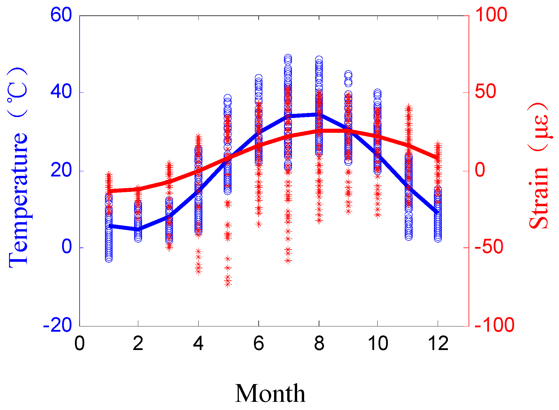
2.2. Monitoring Data and Statistical Analysis of the Temperature and Structure Response

The steel box girder of the investigated bridge is longer in the longitudinal direction compared to the lateral and vertical directions. Additionally, the longitudinal curvature is small, and the cross-section along the longitudinal direction changes uniformly. Therefore, it is assumed that the thermal field along the longitudinal direction of the bridge is consistently exposed to solar radiation and atmospheric temperature. The lateral and vertical temperature distribution of the STB steel box girder is focused. Previous studies have found that the temperatures at the top and bottom plates of the bridge remain consistent along the longitudinal direction, while the temperatures at the web, which is the vertical component connecting the top and bottom plates, show variations between the upstream and downstream of the bridge [41]. However, the analysis of the STB temperature monitoring data does not reveal any temperature gradient along the lateral direction of the top plate. The same observation holds for the bottom plate, top plate U-ribs and bottom plate U-ribs. Moreover, the web temperatures at both sides are the same as shown in Figure 3a, which is different from previous research results. The temperatures of diaphragms are consistent with those of the webs. This is because the tuyere, as a non-structural component, is directly exposed to solar radiation, while the diaphragm and the web are located inside of the tuyere and are not directly affected by solar radiation. The girder without the tuyere component generally exhibits a temperature gradient in the lateral direction. However, after the tuyere is installed, the web is not directly exposed to the sun, resulting in the disappearance of the lateral temperature gradient. Figure 3b presents the vertical temperature distribution of the mid-span cross-section. The components are arranged sequentially from high to low temperatures, namely, the top plate, top plate U-rib, diaphragm, bottom plate U-rib and bottom plate, respectively. Figure 3c illustrates the cross-section temperature gradient data, which are compared with the BS 5400 code. According to the data collected by the temperature sensor, the measured temperatures of the top plate and the top plate U-ribs comply with BS 5400, while the measured temperatures of the diaphragm and U-ribs of the bottom plate exceed the values specified by BS 5400. This raises potential concerns for the structural design of the bridge and requires more attention. Based on the above statistical analysis, the thermal field of the STB can be analyzed using a 1D vertical thermal field approach.

The temperature-induced displacement of the girder on the STB is typically related to the average temperature [42]. Figure 4a shows a significant correlation between the average displacement and average temperature. As the girder temperature increases, the displacement also increases, and vice versa. However, this trend is not consistently observed. There is a time delay effect in which the temperature data lag behind the displacement data for a certain period. Perhaps this is because the temperature sensors are installed inside the steel box girder, and it takes a certain time for the heat to transfer to the thermometers. The time delay effect between the structural displacement response and the temperature load on the STB is approximately one hour. Figure 4b presents the correlation between the average temperature difference ∆T and the average displacement difference ${\delta }_u$. Both values are calculated as the differences from their initial values. The correlation does not follow a linear relationship. The nonlinear relationship is mainly attributed to the time delay effect. By considering the time delay effect and shifting the temperature axis in the negative direction, a linear relationship between displacement and temperature can be observed (Figure 4c).

It is shown in Table 1 that there is a significant correlation between temperature and temperature-induced strain for a single day. Owing to the temperature of the top plates being higher than the bottom plates, the top plates (S-5-2, 4 and 6) represent compression, while the bottom plates (S-5-7 and 9) exhibit tension. The compressive strain of top plates increases continuously with increasing temperature, and vice versa. For instance, if the temperature rises by 20 °C, the compressive strain of the top plate increases to 60 με. On the other hand, the tensile strain of bottom plates increases continuously with the rising temperature, and vice versa. When the temperature increment of the bottom plate reaches 7 °C, the tensile strain of the bottom plate increases to 80 με. However, the temperature-induced strain of the U-ribs is influenced by the combined temperature of the decks and U-ribs. Between 10:00 and 15:00, the top plate U-ribs are under tension. In other time periods, the top plate U-ribs are under compression. This phenomenon occurs because the temperature of the top plates is higher than the top plate U-ribs between 10:00 and 15:00. Therefore, the top plates exhibit compression and the top plate U-ribs exhibit tension. However, the bottom plate U-ribs are under tension throughout.

Figure 5 shows the correlation between temperature and longitudinal temperature-induced strain of the girder under the influence of seasonal temperature variations in one year. The temperature and longitudinal strain were obtained from the temperature sensor T-5-5 and strain gauge S-5-5 on the top plate of the mid-span section on the STB. Firstly, the temperature and longitudinal strain of the first three days of each month were selected as representative data, and the data for each hour were averaged. Then, the monthly temperature and longitudinal strain data were averaged, respectively, resulting in a total of 12 monthly average temperature and 12 monthly average strain data points. The results indicate a sinusoidal relationship between seasonal temperature and longitudinal strain within a year. The top plate temperature reached its maximum value in August and its minimum value in February. On the other hand, the top plate strain reached its maximum value in September and its minimum value in February.

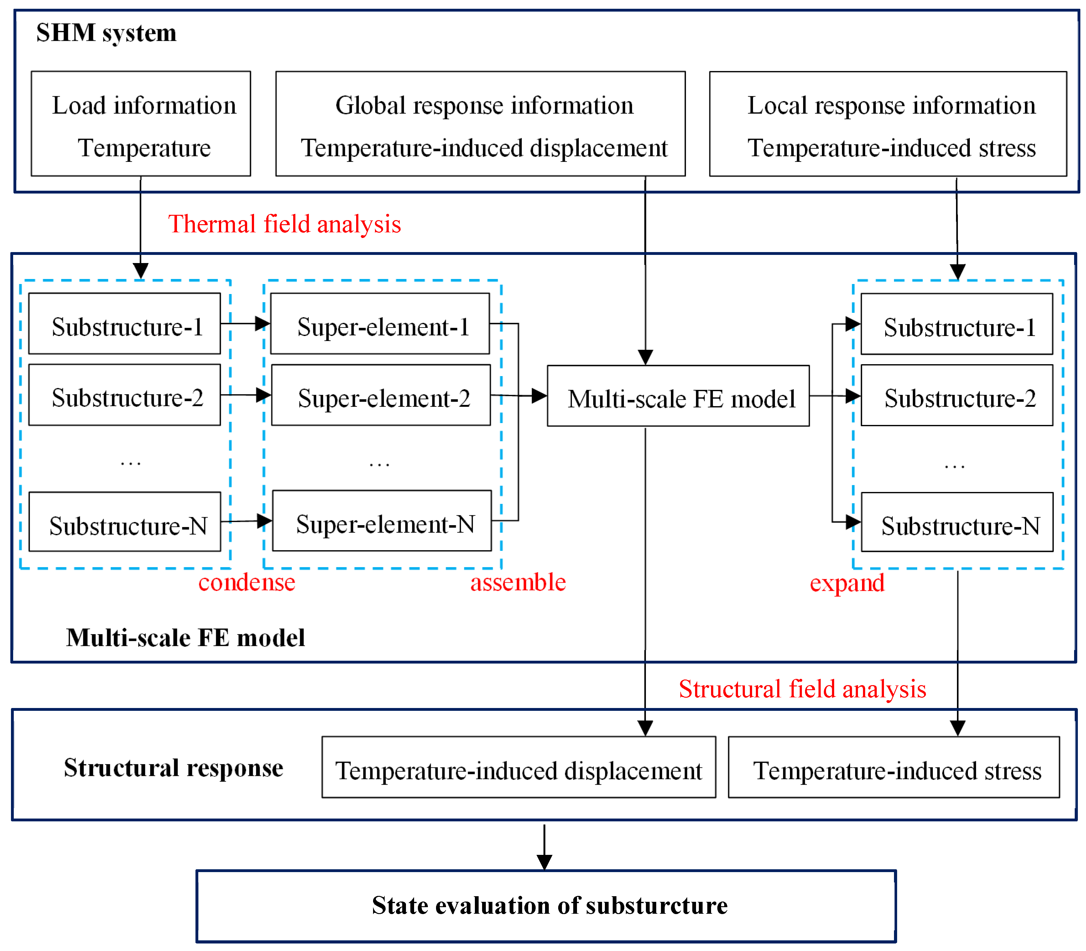
3. Analysis of Temperature-Induced Stress through Multi-Scale Modelling

3.1. STB Multi-Scale Modelling Using the Substructure Method

By providing both global and local information to assess the structural safety performance, the multi-scale FE model can not only be used to perform static and dynamic analysis at the global level but also can analyze the stress of local components such as local strain, fatigue and the fracture of cracks.

The STB multi-scale FE model was established through ANSYS. Figure 6a shows the division of the girder into segments on the STB. The segment among the stay cables is selected as a segment model considering the connections between the girder, cables, towers and piers. The diaphragm enhances the load-bearing capacity of the segment at the end of the girder and the segment at the tower. Each segment is considered a substructure. Accordingly, the segment with a longitudinal length of 6.7 m is divided into a substructure GEN3, located at the end of the girder; the segment between stay cable No.2, with a longitudinal length of 48 m, is divided into a substructure GEN2, located at the tower; the standard segment between the adjacent stay cables, with a longitudinal length of 16 m, is divided into a substructure GEN0 and the standard segment between the contiguous stay cable with a longitudinal length of 12 m, is divided into a substructure GEN01. As the longitudinal truss of the mid-span segment is designed differently from the standard segment GEN0, it was divided into a single substructure GEN1. Overall, there are 53 standard segment substructures GEN0, 11 standard segment substructures GEN01, 1 mid-span segment substructure GEN1, 1 segment substructure GEN2 under the tower, and 1 segment substructure GEN3 at the end of the girder, all positioned on the side of the symmetrical axis on the STB. Figure 6d presents the FE model of the segment substructure GEN1 on the STB, modeled according to the design drawing. The segment, including top plates, bottom plates, webs, diaphragms and U-ribs, is simulated through the SHELL63 shell element in ANSYS. The top and bottom flanges of the longitudinal truss are welded with the top and bottom plates by steel plates, and thus the SHELL63 element is used to simulate the top and bottom flanges. The diagonal braces of the longitudinal truss adopt angle steel, and therefore, the BEAM4 element is used to simulate the longitudinal braces.

In the STB multi-scale FE model, each segment substructure model (Figure 6c) should be condensed into a super-element (Figure 6b), which is the condensation of a group of elements into one element using the substructure method. The purpose of this condensation is to simplify the model and improve computational efficiency. Once the super-element matrices have been formed, they are stored in a file and can be used as normal finite elements in subsequent analyses. The master nodes (purple nodes in Figure 6c) are selected to connect segment models and the other components in the multi-scale FE model. In the substructure model, all nodes (with the exception of the master nodes) are eliminated through the substructure technique. More specifically, a group of elements is condensed into one super-element, with representative nodes of the segment model interface selected as the master nodes. In the case of segment substructure model GEN2, three additional rows of master nodes are additionally selected based on the connection of the beam between the substructure and tower, as well as the connection between the substructure and stay cable No.1. The DOFs of the master nodes on the interface of each segment substructure were then coupled.

Owing to the length of the girder being long, the mass block was used inside the steel box girder at the piers to endure the warping deformation of the girder at these locations. The mass block was simulated by structural mass element MASS21 at the corresponding master nodes. In addition, the secondary dead load exerts a great impact on the static and dynamic performance of the bridge structures and is non-negligible. The secondary dead load of the STB deck was also simulated via MASS21. Based on the design drawing, the secondary dead loads of the bridge deck were converted into the mass of the MASS21 elements. The girder model was built following the completion of all the above steps.

The tower and pier of the STB were modeled by the 3D beam element BEAM188, which could accurately simulate the hollow cross-section characteristics of the concrete structure. Nonlinear truss element LINK10 was employed to simulate the stay cable, which was set to tension-only. The stay cable force of the bridge design was converted into the initial strain to simulate the initial tension of the stay cables. The stay cable experiences sag due to its self-weight, and cannot be calculated using the tensile truss element. In this case, the sag effect needs to be considered by the equivalent elasticity modulus. The Ernst formula (Equation (1)), initially proposed by German scholar Ernst in 1965, is widely used for this purpose. The formula assumes that the cable weight is uniformly distributed along chord length (not arc length) and neglects the cable’s ability to bear bending moments. As a result, the shape of the stay cable follows a parabolic curve.

$$E_l=\frac{E_e}{1+\frac{E_e{\gamma }^2{l}_x^2}{12{\sigma }^3}}$$

(1)

where $E_l$ is the corrected elastic modulus of the stay cable; $E_e$ is the initial elastic modulus of the stay cable; $\sigma$ is the stress of the stay cable; $\gamma$ is the unit weight of the stay cable; $l_x$ is the horizontal projection length of the stay cable.

As STB bearings in the piers constrain the transverse and vertical displacement of the girder, these constraints were used at the joints between the piers and the girder. With the presence of the support beam between the tower and the girder, constraints were used to connect the support beam and the girder. The foundation at the bottom of the towers and three piers were constrained by fixed constraints. The multi-scale FE model was developed by coupling the master node DOFs on the girder super-elements with the nodes on stay cables, towers, and piers. Figure 5b presents the assembly of the STB multi-scale model by various components.

The proposed model was verified using SHM data prior to its application for the temperature-induce response analysis. The results obtained from the modal analysis of the multi-scale FE model were compared with measured values reported by Zhang and Chen [43]. The first three order modes of the multi-scale FE model were identified as the first-order longitudinal mode, the first-order symmetric lateral bending mode and the first-order symmetric vertical bending mode, with corresponding frequencies of 0.0693, 0.1069, 0.1884 Hz, respectively. By comparing with the frequency in the reference [43], the errors are determined as 8.1%, 5.3%, and 3.5%, respectively. The values calculated with the proposed method are consistent with the test values, indicating the proposed modeling strategy is reliable and the model can be adopted for further analysis.

The above models can be directly applied to stress field analysis. However, it is necessary to investigate the thermal field analysis before analyzing the temperature-induced displacement/stress. Since the longitudinal thermal variation of the bridge is not obvious, only the thermal field analysis of segment substructures with different geometry features was carried out. The thermal field was calculated using the heat-transfer analysis on the segment substructures GEN0, GEN01, GEN1, GEN2 and GEN3, which had not yet been condensed into super-elements. The structural elements should be replaced by thermal elements. The 3D thermal shell element SHELL57 replaced the elastic shell element SHELL63. Similarly, the convection link element LINK34 was used instead of the 3D elastic beam element BEAM4. The bridge deck pavement has a great influence on the results of thermal field analysis. Therefore, the SOLID70 thermal solid element was employed to simulate the bridge deck pavement, which is made up of 5.5 cm thick epoxy asphalt concrete on the bridge deck. During the thermal field analysis, the secondary dead load was deleted. When the stress field model was analyzed, the temperature results calculated by the thermal field were substituted into the segment substructures GEN0, GEN01, GEN1, GEN2 and GEN3 as the element internal force, and then each segment substructure was condensed into a super-element.

The advantages of the multi-scale FE model were illustrated by comparing with the global fine FE model. As shown in

Table 2. Comparison of calculation scale and time between thermal field models.

	Nodes	Elements	DOFs	Thermal Analysis Time (s)
global fine	1,690,000	2,359,862	11,274,550	625,920
multi-scale	78,620	94,395	471,720	25,180

, the DOFs of the global fine FE model are 11,274,550, while the DOFs of the multi-scale FE thermal field model proposed in this paper are only 471,721. Based on the ANSYS run-time stats module, the number of the nodes, elements and DOFs of the global fine thermal field FE model is about 22 times, 25 times and 24 times that of the multi-scale FE model, respectively, and the time required for thermal analysis is about 25 times longer. As shown in

Table 3. Comparison of calculation scale and time between stress field models.

	Nodes	Elements	DOFs	Static Time (s)	Stress Analysis Time (s)
global fine	1,690,000	2,359,862	11,274,550	26,080	625,920
multi-scale	14,955	1035	69,272	16	15,491

, the DOFs of the global fine stress field FE model are 11,274,550, while the DOFs of the multi-scale FE model proposed in this paper are only 69,272. The number of nodes, elements and DOFs of the global fine stress field FE model is approximately 113 times, 2280 times and 162 times that of the multi-scale FE model, respectively, and the time required for static self-balance analysis (under the action of gravity load and measured cable force, the calculated value of girder deformation is consistent with the measured value) and temperature-induced stress analysis is about 1630 times and 40 times longer. Therefore, if the global fine FE method is used to analyze the temperature-induced strain of U-ribs, the model has a significantly large number of DOFs, leading to the consumption of extensive hardware resources and calculation time, and in some cases, it may not even be feasible to perform the calculation. However, the multi-scale FE model analysis can save a significant amount of computing time on the premise of accuracy, which is convenient for subsequent parameter analysis and structural performance evaluation.

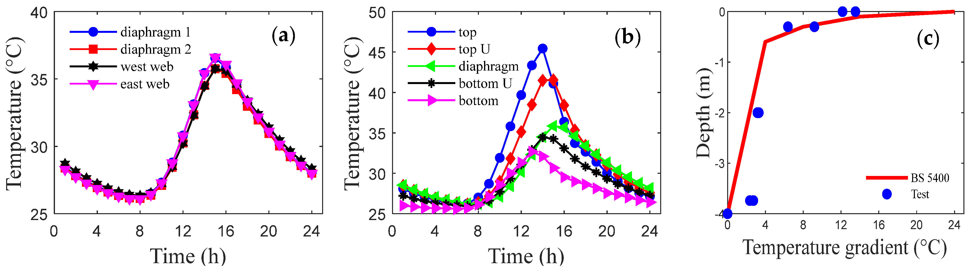
3.2. Thermal Field Analysis

The thermal parameters of the steel components and deck pavement asphalt concrete, including thermal conductivity, specific heat capacity and density, were determined as shown in

Table 4. Thermal parameters of material.

	Steel	Asphalt
thermal conductivity $k$ ($\mathrm{W}/(\mathrm{m}·\mathrm{K})$)	60.5	2
heat capacity $c \left(\frac{\mathrm{J}}{\mathrm{k}\mathrm{g}·\mathrm{K}}\right)$	460	900
density $\rho$ ($\mathrm{k}\mathrm{g}/{\mathrm{m}}^3$)	7850	2100

[44,45,46]. Generally, the atmospheric temperature one hour before sunrise is considered the initial temperature of the bridge. The temperature distribution inside and outside the STB box girder at 6:00 a.m. is relatively uniform, so it is appropriate to take the atmospheric temperature at 6:00 a.m. as the initial atmospheric temperature. The time interval for the thermal field analysis is set to one hour.

Thermal field analysis was performed to determine the boundary conditions, including absolute radiation temperature $T_v$ and overall heat transfer coefficient $h_o$. The relation between the radiation and reflection balance of the deck surface on the bridge is described as Equation (2) [44]:

$$q_B+q_k=q_J+q_H+q_R+q_{G_a}+q_{UR}$$

(2)

where $q_B$ is the structural radiation; $q_k$ is the thermal irradiation; $q_J$ is the solar direct radiation; $q_H$ is the scattered radiation; $q_R$ is the reflected radiation; $q_{G_a}$ is the atmospheric radiation and $q_{UR}$ is the surface effective radiation. The equations for the above parameters can be found in reference [45].

Equation (2) is a fourth-order transcendental equation of $T_v$ and cannot be solved directly. Therefore, the following formula is used to simplify the equation [45]:

$${\epsilon }_{bl}{C}_s{T}_v{}^4=h_r\left(T_v-T_a\right)+{\epsilon }_{bl}{C}_s{T}_a{}^4$$

(3)

where ${\epsilon }_{bl}$ is the structural radiation coefficient; $C_s$ is the Stefan–Boltzmann constant, $C_s=5.677\times {10}^{-4} {\mathrm{W}/\mathrm{m}}^2{\mathrm{K}}^4$; $T_a$ is the atmospheric temperature; $h_o=h_r+h_k$, $h_r$ is the coefficient of radiation heat transfer and $h_v$ is the exchange heat transfer coefficient.

The absolute radiation temperature $T_v$ can be determined as the following formulas [45]:

$$\{\begin{array}{l}{T}_{v,top}=T_a+\frac{a_{bk}}{h_r+h_k}\left(I_{J}sinh+I_H\right)-\left(1-{\epsilon }_a\right)\frac{{\epsilon }_{bl}{C}_s}{h_r+h_k}{T}_a{}^4\\ T_{v,bot}=T_a+\frac{{\gamma }_{uk}{a}_{bk}}{h_r+h_k}\left(I_{J}sinh+I_H\right)\\ T_{v,web}=T_a+\frac{a_{bk}}{h_r+h_k}[{\gamma }_{uk}\left(I_{J}sinh+I_H\right)co{s}^2\frac{\beta }{2}+I_{H}cos\left(\frac{\pi }{2}+h-\beta \right)\\ cos\left(\alpha -{\alpha }_w\right)sinh+I_{H}si{n}^2\frac{\beta }{2}]-\left(1-{\epsilon }_a\right)\frac{{\epsilon }_{bl}{C}_s}{h_r+h_k}{T}_a{}^{4}si{n}^2\frac{\beta }{2}\end{array}$$

(4)

where $T_v$ includes $T_{v,top}$, $T_{v,bot}$ and $T_{v,web}$. $T_{v,top}$ is the absolute radiation temperature of the top plate; $T_{v,bot}$ is the absolute radiation temperature of the bottom plate; $T_{v,web}$ is the absolute radiation temperature of the web; $a_{bk}$ is the shortwave radiation absorptivity; $h$ is solar altitude angle; ${\epsilon }_a$ is the atmospheric radiation coefficient, ${\epsilon }_a=0.82$; ${\gamma }_{uk}$ is the ground reflection coefficient; $I_J$ is the direct solar radiation intensity and $I_H$ is the solar scattered energy; $\beta$ is included angle between web and horizontal plane; $\alpha$ is the azimuth of the sun, which is the included angle between the projection of the line from the observer to the sun on the ground plane and the due south direction; ${\alpha }_w$ is the azimuth of the external normal of the web. The steel and asphalt shortwave radiation absorptivity were considered to be 0.685 and 0.9, and the steel and asphalt surface radiation coefficients were assumed to be 0.8 and 0.92, respectively [44]. For more detailed information on these expressions, please refer to [45].

Based on the measured meteorological data and calculation parameters of the thermal field, the thermal boundary conditions were calculated by Equation (4). Then these boundary conditions were applied to the segment substructures for transient thermal analysis. Figure 7 presents the thermal field of the substructure GEN1 calculated for one day. Through conducting statistical analysis of the errors between calculated and measured values, it was found that the maximum error of temperature for the top plate is 8.2%, and the weighted average error within a day is 3.9%. The maximum error and the weighted average error for the bottom plate are 7.8% and 3.5%, respectively. For the web, corresponding values are 7.1% and 3.5%, respectively. For the diaphragm, they are 5.6% and 4.1%, respectively. For the top plate U-rib, they are 9.9% and 6.2%, respectively. For the bottom plate U-rib, they are 5.0% and 2.1%, respectively. There is an agreement between the predicted and measured temperatures. This verifies the effectiveness of the numerical model and the heat transfer analysis.

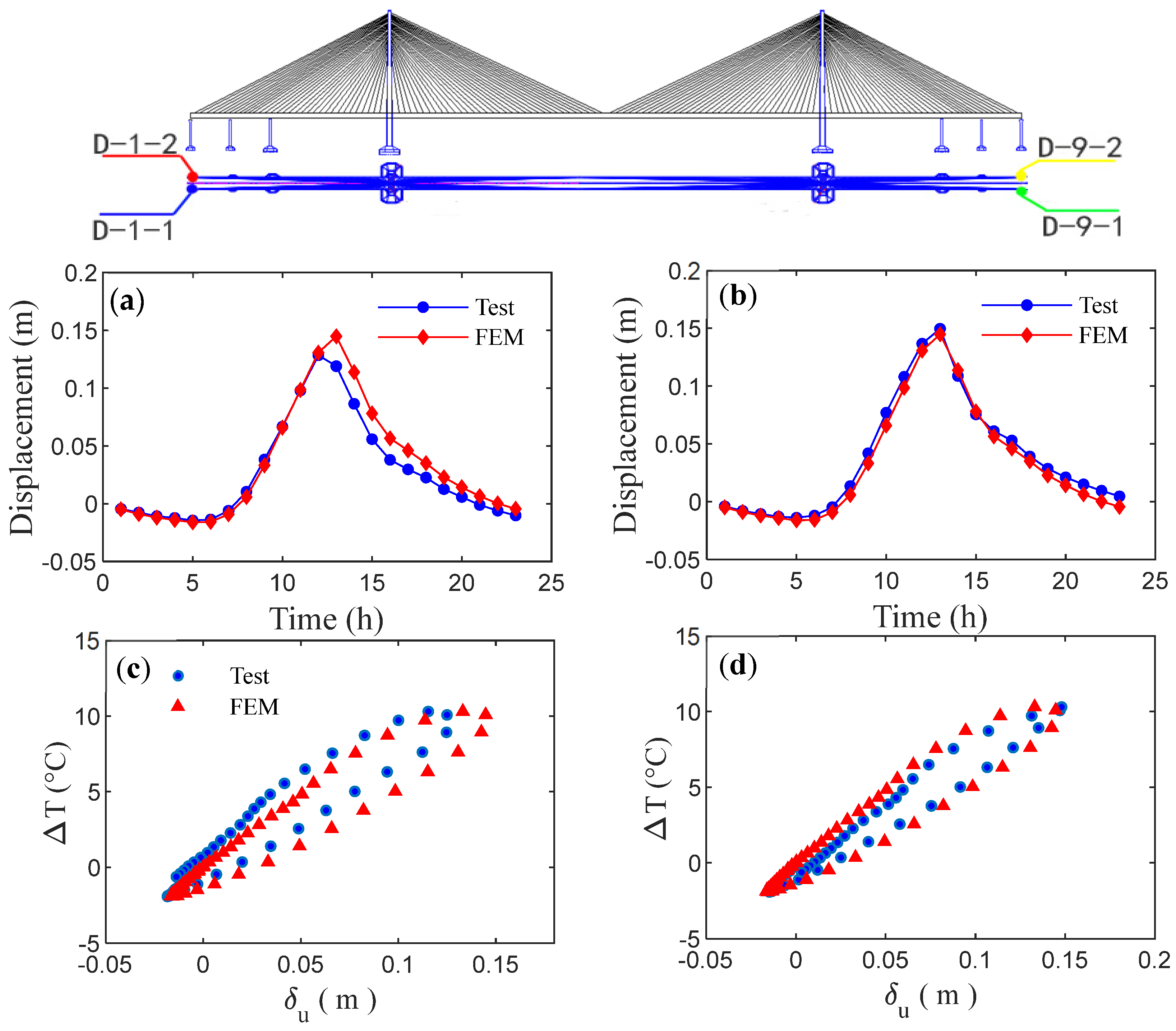
3.3. Temperature-Induced Structural Responses

The temperature-induced responses can be investigated by combing the temperature time history with the multi-scale FE stress field model. In this section, the focus is on the analysis of longitudinal temperature-induced displacements at the end of the girder and the longitudinal temperature-induced strains on the sensor layout cross-section. First, the results of thermal field analysis are imported into each segment substructure model (Figure 6c) and then the temperature load is treated as the internal force, each segment substructure model is condensed into a super-element (Figure 6b); at last, these super-elements are applied to the multi-scale FE model for stress field analysis. The isotropic linear constitutive model for thermal expansion is adopted. Temperature-induced displacement can be directly calculated from the master nodes of the girder end in the multi-scale FE model. Figure 8a,b depicts the temperature-induced displacements at the end of the girder. The calculated values of the FE model are in agreement with the measured values of the D-9-1 displacement gauges. However, there is a certain deviation between the temperature-induced displacements of the D-1-1 displacement gauges and the calculated values. It should be noted that the STB multi-scale FE model is assumed symmetry with respect to the mid-span cross-section of the girder, resulting in consistent displacements calculated by the FE model on both sides. However, this assumption does not match the actual situation. Figure 8c,d displays the correlation between the temperature and temperature-induced displacements. The statistical results indicate the accuracy of the correlation between temperature and temperature-induced displacement based on the proposed method.

The temperature-induced displacement can be calculated directly. However, in order to obtain the temperature-induced stress and strain, an additional step is required. At first, it is necessary to reverse the displacement of the master nodes back to the segment substructure to calculate the displacement of the slave nodes; then the element temperature-induced stress and strain in the segment substructure are calculated based on the displacement of the slave node. Figure 9 shows that the calculated values of decks and U-ribs are consistent with the measured values. Equation (5) is used as an evaluation indicator to compare the calculated and measured values of temperature-induced strain. The evaluation indicator value ranges between 0 and 1, with a value closer to 1 indicating a better similarity between the two sets of values.

$$I=\frac{{\left|{{\displaystyle \sum }}_{i=1}^n{S}_{ai}{S}_{ei}\right|}^2}{\left({{\displaystyle \sum }}_{i=1}^n{S}_{ai}{S}_{ai}\right)\left({{\displaystyle \sum }}_{i=1}^n{S}_{ei}{S}_{ei}\right)}$$

(5)

where $I$ is the evaluation indicator, $S_{ai}$ is the calculated value of temperature-induced strain for i-th sampling point, $S_{ei}$ is the measured value of temperature-induced strain for i-th sampling point, $n$ is the number of samples for one day.

The evaluation indicator values for S-5-1 to S-5-6 in the top plate or top plate U-rib are 0.96, 0.97, 0.94, 0.95, 0.75 and 0.98, respectively. The evaluation indicator values for S-5-8 to S-5-10 in the bottom plate or bottom plate U-rib are 0.90, 0.77 and 0.93, respectively. Therefore, compared with the traditional FE model, the multi-scale FE model based on the substructure method can be adopted to analyze the temperature-induced stress of the local members (i.e., U-ribs) on long-span bridges.

In order to evaluate the variations in the strain distribution across the longitudinal and vertical directions of the girder cross-section for one day, strains at different cross-sections and positions were analyzed at 6:00 and 14:00, respectively. Figure 10a shows that the top plates (SA-N-1, 3, 5) are subject to compression, while the bottom plates (SA-N-2, 4, 6) suffer from tension at 14:00. Moreover, the girder exhibits an upward bending behavior. However, the inverse phenomenon is observed in Figure 10b, whereby the top and bottom deck are subject to tension and compression, respectively, at 6:00, and the girder exhibits a downward bending behavior. Similar strain trends are observed at the top and bottom plate U-ribs in Figure 10c,d, respectively. This is attributed to the greater temperature of the top girder compared to the bottom girder at 14:00, while an inverse temperature distribution along the vertical direction is present at 6:00. The maximum variation range of the temperature-induced strain at the top plate and bottom plate is approximately 100 $\mathsf{\mu }\mathsf{\epsilon }$ over the course of one day.

4. Conclusions

The performance evaluation of OSD by considering the temperature load is very important. In previous studies, the strain of local components needed to be analyzed in the global fine finite FE model. In this paper, based on substructure technology, the temperature-induced stress of U-ribs is evaluated using a multi-scale FE model on a long-span cable-stayed bridge. The following key conclusions are obtained.

(1)

The temperature-induced stress of U-ribs on the STB was analyzed based on monitoring data and the multi-scale FE method. This method can be applied to other long-span bridges to address the issue of low computational efficiency in analyzing U-ribs in the global fine FE model.

(2)

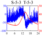
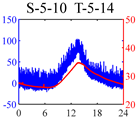
Analysis of monitoring data indicates that the long-span steel box bridge with the tuyere components exhibits a vertical temperature gradient rather than a transverse temperature gradient. The correlation between temperature-induced displacement and temperature demonstrates a linear relationship once the time delay effect is considered. The temperature-induced strain of the top plates and bottom plates is influenced by the temperature between them. The temperature-induced strain of U-ribs is influenced by the temperature of the decks and U-ribs. Furthermore, the seasonal temperature and longitudinal strain over time within a year exhibit a sinusoidal relationship.

(3)

A multi-scale FE model, which can effectively reduce the calculation time based on the substructure method, has been established to analyze the temperature-induced stress of U-ribs on long-span bridges. The accuracy of the multi-scale FE model results for the temperature-induced stress of U-ribs has been confirmed through monitoring data.

(4)

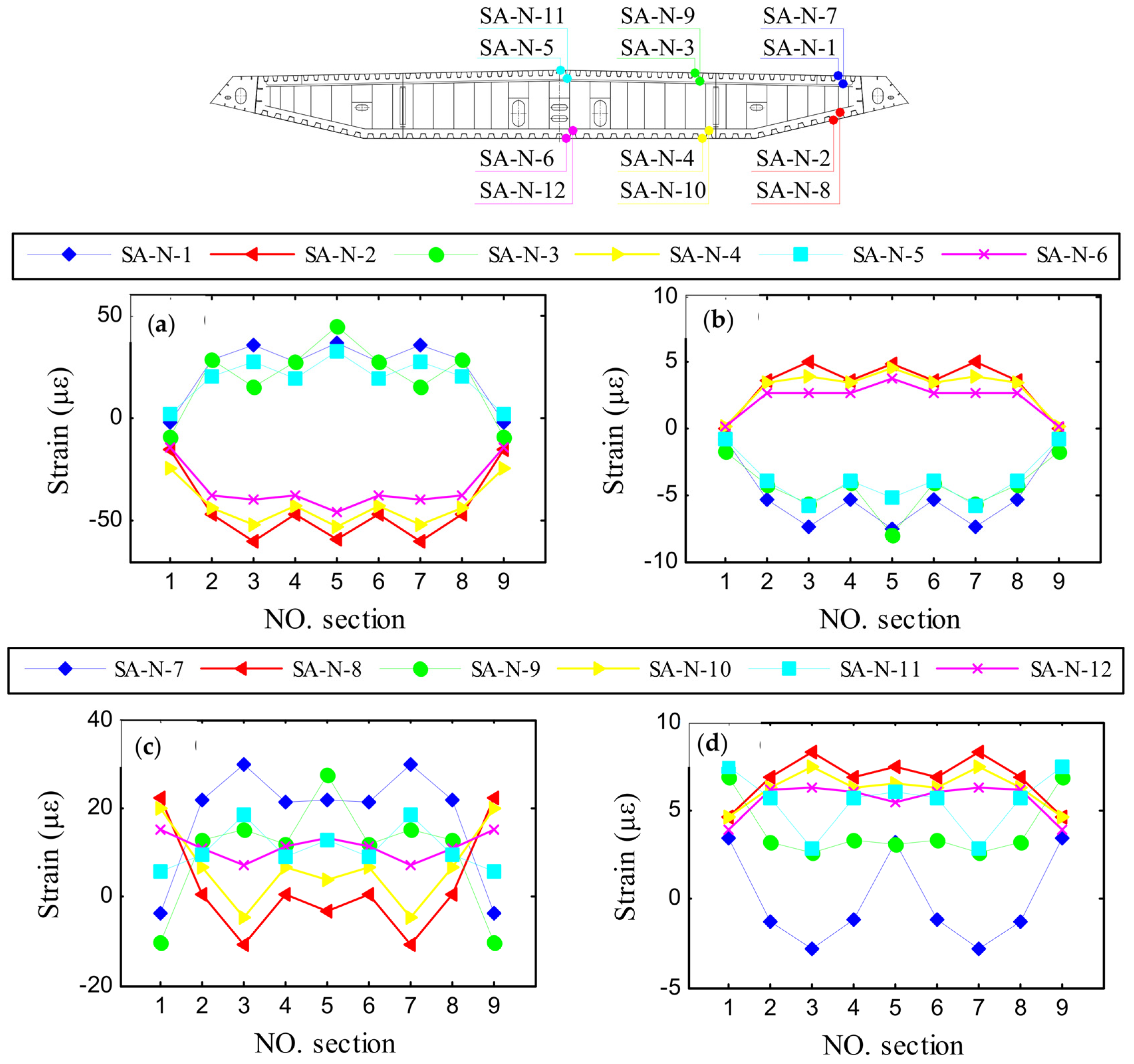
By evaluating the temperature-induced strain during the highest and lowest temperatures of one day on the multi-scale FE model, it indicates that the deflection of the girder, a key index for bridge design and SHM assessment, exhibits dynamic changes in response to temperature loads. The temperature-induced strain of the top and bottom plates displays a maximum variation range of approximately 100 $\mathsf{\mu }\mathsf{\epsilon }$.

5. Recommendation

Due to the limitations of research time, the evaluation and discussion are focused on the longitudinal temperature-induced strain of specific segments on the bridge, specifically the top plate, bottom plate, and U-ribs. In future research, the temperature-induced strain of web plates, diaphragms, and diaphragms can be studied in depth, as well as more segments of the girder. Additionally, it is recommended to investigate the influence of temperature load on the fatigue behavior of U-ribs under varying thermal conditions.

References

1. Zhao, R.; Zheng, K.; Wei, X.; Jia, H.; Liao, H.; Li, X.; Wei, K.; Zhan, Y.; Zhang, Q.; Xiao, L.; et al. State-of-the-art and annual progress of bridge engineering in 2020. Adv. Bridge Eng. 2021, 2, 1–105. [Google Scholar]
2. Zeng, Y.; Qiu, Z.; Yang, C.C.; Haozheng, S.; Xiang, Z.F.; Zhou, J.T. Fatigue experimental study on full-scale large sectional model of orthotropic steel deck of urban rail bridge. Adv. Mech. Eng. 2023, 15, 16878132231155271. [Google Scholar] [CrossRef]
3. Guo, T.; Li, A.Q.; Wang, H. Influence of ambient temperature on the fatigue damage of welded bridge decks. Int. J. Fatigue 2008, 30, 1092–1102. [Google Scholar] [CrossRef]
4. Liu, Y.; Zhang, H.P.; Liu, Y.M.; Deng, Y.; Jiang, N.; Lu, N.W. Fatigue reliability assessment for orthotropic steel deck details under traffic flow and temperature loading. Eng. Fail. Anal. 2017, 71, 179–194. [Google Scholar] [CrossRef]
5. Xia, Q.; Xia, Y.; Wan, H.P.; Zhang, J.; Ren, W.X. Condition analysis of expansion joints of a long-span suspension bridge through metamodel-based model updating considering thermal effect. Struct. Control. Health Monit. 2020, 27, e2521. [Google Scholar] [CrossRef]
6. Xiao, F.; Hulsey, J.L.; Balasubramanian, R. Fiber optic health monitoring and temperature behavior of bridge in cold region. Struct. Control. Health Monit. 2017, 24, e2020. [Google Scholar] [CrossRef]
7. Wang, D.; Liu, Y.M.; Liu, Y. 3D temperature gradient effect on a steel–concrete composite deck in a suspension bridge with field monitoring data. Struct. Control. Health Monit. 2018, 25, e2179. [Google Scholar] [CrossRef]
8. Yarnold, M.T.; Moon, F.L. Temperature-based structural health monitoring baseline for long-span bridges. Eng. Struct. 2015, 86, 157–167. [Google Scholar] [CrossRef]
9. Ni, Y.Q.; Xia, H.W.; Wong, K.Y.; Ko, J.M. In-Service Condition Assessment of Bridge Deck Using Long-Term Monitoring Data of Strain Response. J. Bridge Eng. 2012, 17, 876–885. [Google Scholar] [CrossRef]
10. Xia, Y.Y.; Shi, M.S.; Zhang, C.; Wang, C.X.; Sang, X.X.; Liu, R.; Zhao, P.; An, G.F.; Fang, H.Y. Analysis of flexural failure mechanism of ultraviolet cured-in-place-pipe materials for buried pipelines rehabilitation based on curing temperature monitoring. Eng. Fail. Anal. 2022, 142, 106763. [Google Scholar] [CrossRef]
11. Zuk, W. Simplified Design Check of Thermal Stresses in Composite Highway Bridges; The National Academies of Sciences, Engineering, and Medicine: Washington, DC, USA, 1965; pp. 10–13. [Google Scholar]
12. Peiris, A.; Sun, C.; Harik, I. Lessons learned from six different structural health monitoring systems on highway bridges. J. Low Freq. Noise V. A. 2018, 39, 616–630. [Google Scholar] [CrossRef]
13. Ni, Y.Q.; Xia, Y.; Liao, W.Y.; Ko, J.M. Technology Innovation in Developing the Structural Health Monitoring System for Guangzhou New TV Tower. Struct. Control Health Monit. 2009, 16, 73–98. [Google Scholar] [CrossRef]
14. Deng, Y.; Li, A.Q.; Chen, S.; Feng, D.M. Serviceability assessment for long-span suspension bridge based on deflection measurements. Struct. Control. Health Monit. 2018, 25, e2254. [Google Scholar] [CrossRef]
15. Yuan, J.; Gan, Y.X.; Chen, J.; Tan, S.M.; Zhao, J.T. Experimental research on Consolidation creep characteristics and microstructure evolution of soft soil. Front. Mater. 2023, 10, 1137324. [Google Scholar] [CrossRef]
16. Yang, Z.Y.; Yu, X.Y.; Dedman, S.; Rosso, M.; Zhu, J.M.; Yang, J.Q.; Xia, Y.X.; Tian, Y.C.; Zhang, G.P.; Wang, J.Z. UAV remote sensing applications in marine monitoring: Knowledge visualization and review. Sci. Total Envrion. 2022, 838, 155939. [Google Scholar] [CrossRef]
17. Zhang, B.; Zhou, L.; Zhang, J. A methodology for obtaining spatiotemporal information of the vehicles on bridges based on computer vision. Comput. Aided Civ. Inf. 2018, 34, 471–487. [Google Scholar] [CrossRef]
18. Zhao, W.; Guo, S.; Zhou, Y.; Zhang, J. A Quantum-Inspired Genetic Algorithm-Based Optimization Method for Mobile Impact Test Data Integration. Comput. Aided Civ. Inf. 2018, 33, 411–422. [Google Scholar] [CrossRef]
19. Wang, G.X.; Ye, J.H. Localization and quantification of partial cable damage in the long-span cable-stayed bridge using the abnormal variation of temperature-induced girder deflection. Struct. Control Health Monit. 2019, 26, e2281. [Google Scholar] [CrossRef] [Green Version]
20. Salcher, P.; Pradlwarter, H.; Adam, C. Reliability assessment of railway bridges subjected to high-speed trains considering the effects of seasonal temperature changes. Eng. Struct. 2016, 126, 712–724. [Google Scholar] [CrossRef]
21. Siringoringo, D.M.; Fujino, Y. Seismic response of a suspension bridge: Insights from long-term full-scale seismic monitoring system. Struct. Control Health Monit. 2018, 25, e2252. [Google Scholar] [CrossRef]
22. Xia, Q.; Cheng, Y.Y.; Zhang, J.; Zhu, F.Q. In-Service Condition Assessment of a Long-Span Suspension Bridge Using Temperature-Induced Strain Data. J. Bridge Eng. 2017, 22, 04016124. [Google Scholar] [CrossRef]
23. Xia, Q.; Zhang, J.; Tian, Y.D.; Zhang, Y. Experimental Study of Thermal Effects on a Long-Span Suspension Bridge. J. Bridge Eng. 2017, 22, 04017034. [Google Scholar] [CrossRef]
24. Yu, S.; Li, D.S.; Ou, J.P. Digital twin-based structure health hybrid monitoring and fatigue evaluation of orthotropic steel deck in cable-stayed bridge. Struct. Control Health Monit. 2022, 29, e2976. [Google Scholar] [CrossRef]
25. Yu, S.; Ou, J.P. Fatigue life prediction for orthotropic steel deck details with a nonlinear accumulative damage model under pavement temperature and traffic loading. Eng. Fail Anal. 2021, 126, 105366. [Google Scholar] [CrossRef]
26. Asadollahi, P. Bayesian-Based Finite Element Model Updating, Damage Detection, and Uncertainty Quantification for Cable-Stayed Bridges. Ph.D. Thesis, University of Kansas, Lawrence, KS, USA, 2018. [Google Scholar]
27. Mensah-Bonsu, P.O. Computer-Aided Engineering Tools for Structural Health Monitoring under Operational Conditions. Master’s Thesis, University of Connecticut Graduate School, Storrs, CT, USA, 2012. [Google Scholar]
28. Wang, F.Y.; Xu, Y.L.; Zhan, S. Multi-scale model updating of a transmission tower structure using Kriging meta-method. Struct. Control Health Monit. 2017, 24, e1952. [Google Scholar] [CrossRef]
29. Li, Z.; Chen, Y.; Shi, Y. Numerical failure analysis of a continuous reinforced concrete bridge under strong earthquakes using multi-scale models. Earthq. Eng. Eng. Vib. 2017, 16, 397–413. [Google Scholar] [CrossRef]
30. Kojic, M.; Milosevic, M.; Kojic, N.; Starosolski, Z.; Ghaghada, K.; Serda, R.; Annapragada, A.; Ferrari, M.; Ziemys, A. A multi-scale FE model for convective-diffusive drug transport within tumor and large vascular networks. Comput. Method Appl. M. 2015, 294, 100–122. [Google Scholar] [CrossRef]
31. Pletz, M.; Daves, W.; Yao, W.; Kubin, W.; Scheriau, S. Multi-scale FE modeling to describe rolling contact fatigue in a wheel-rail test rig. Tribol. Int. 2014, 80, 147–155. [Google Scholar] [CrossRef]
32. Trofimov, A.; Le-Pavic, J.; Ravey, C.; Albouy, W.; Therriault, D.; Levesque, M. Multi-scale modeling of distortion in the non-flat 3D woven composite part manufactured using resin transfer molding. Compos. Part A. 2021, 140, 106145. [Google Scholar] [CrossRef]
33. Chen, L.; Qian, Z.; Wang, J. Multiscale Numerical Modeling of Steel Bridge Deck Pavements Considering Vehicle-Pavement Interaction. Int. J. Geomech. 2016, 16, B4015002. [Google Scholar] [CrossRef]
34. Chan, T.H.T.; Li, Z.X.; Ko, J.M. Fatigue analysis and life prediction of bridges with structural health monitoring data—Part II: Application. Int. J. Fatigue 2001, 23, 55–64. [Google Scholar] [CrossRef]
35. Li, Z.X.; Jiang, F.F.; Tang, Y.Q. Multi-scale analyses on seismic damage and progressive failure of steel structures. Finite Elem. Anal. Des. 2012, 48, 1358–1369. [Google Scholar] [CrossRef]
36. Nie, J.; Zhou, M.; Wang, Y.; Fan, J.; Tao, M. Cable Anchorage System Modeling Methods for Self-Anchored Suspension Bridges with Steel Box Girders. J. Bridge Eng. 2014, 19, 172–185. [Google Scholar] [CrossRef]
37. Wang, F.; Xu, Y.; Sun, B.; Zhu, Q. Updating Multiscale Model of a Long-Span Cable-Stayed Bridge. J. Bridge Eng. 2018, 23, 04017148. [Google Scholar] [CrossRef]
38. Jensen, H.A.; Munoz, A.; Papadimitriou, C.; Vergara, C. An enhanced substructure coupling technique for dynamic re-analyses: Application to simulation-based problems. Comput. Method Appl. M. 2016, 307, 215–234. [Google Scholar] [CrossRef]
39. Li, Z.X.; Chan, T.H.T.; Yu, Y.; Sun, Z.H. Concurrent multi-scale modeling of civil infrastructures for analyses on structural deterioration-Part I: Modeling methodology and strategy. Finite Elem. Anal. Des. 2009, 45, 782–794. [Google Scholar] [CrossRef]
40. Zhu, Q.; Xu, Y.L.; Xiao, X. Multiscale Modeling and Model Updating of a Cable-Stayed Bridge. I: Modeling and Influence Line Analysis. J. Bridge Eng. 2015, 20, 04014112. [Google Scholar] [CrossRef]
41. Roberts-Wollman, C.L.; Breen, J.E.; Cawrse, J. Measurements of Thermal Gradients and their Effects on Segmental Concrete Bridge. J. Bridge Eng. 2002, 7, 166–174. [Google Scholar] [CrossRef]
42. Specifications ALBD. Final Report of the AASHTO Standing Committee on Highways Task Force on Commercialization of Interstate Highway Rest Areas; American Association of State Highway and Transportation Officials (AASHTO): Washington, DC, USA, 2007. [Google Scholar]
43. Zhang, X.G.; Chen, A.R. Design and Structural Performance of Sutong Bridge; CnDao: Beijing, China, 2010. [Google Scholar]
44. Xia, Y.; Chen, B.; Zhou, X.Q.; Xu, Y.L. Field monitoring and numerical analysis of Tsing Ma Suspension Bridge temperature behavior. Struct. Control Health Monit. 2013, 20, 560–575. [Google Scholar] [CrossRef]
45. Kehlbeck, F. Influence of Solar Radiation on Bridge Structure; China Communication Press: Beijing, China, 1981. [Google Scholar]
46. Zhou, L.R.; Xia, Y.; Brownjohn, J.M.W.; Koo, K.Y. Temperature Analysis of a Long-Span Suspension Bridge Based on Field Monitoring and Numerical Simulation. J. Bridge Eng. 2016, 21, 04015027. [Google Scholar] [CrossRef]
Figure 1. Framework of U-ribs state evaluation through multi-scale FE model and monitoring data.
Sustainability 15 09149 g001
Figure 2. The cable-stayed bridge and its SHM system. (a) bridge image (b) components of steel girder (c) sensor layout.
Sustainability 15 09149 g002
Figure 3. Temperature distribution. (a) lateral direction (b) vertical direction (c) temperature gradient.
Sustainability 15 09149 g003
Figure 4. Temperature-Displacement correlation analysis. (a) time-delay effect (b) without considering time-delay (c) considering time-delay.
Sustainability 15 09149 g004
Figure 5. Temperature-induced strain correlation analysis in a year.
Sustainability 15 09149 g005
Figure 6. Multi−scale modeling. (a) segment substructure division (b) multi−scale FE model and super-elements (c) segment substructure models (d) modeling details of GEN1.
Sustainability 15 09149 g006
Figure 7. Comparison of thermal field measured and calculated values of each component on substructure GEN1. (a) top plate, (b) bottom plate, (c) web, (d) diaphragm, (e) top plate U-rib, (f) bottom plate U-rib.
Sustainability 15 09149 g007
Figure 8. Comparison between calculated displacements and measured values. (a) D-1-1 displacement history, (b) D-9-1 displacement history, (c) D-1-1 temperature-displacement correlation, (d) D-9-1 temperature-displacement correlation.
Sustainability 15 09149 g008
Figure 9. Calculated structural strain response.
Sustainability 15 09149 g009
Figure 10. Longitudinal and vertical distributions of strain. (a) Strain distribution of plates at 14:00, (b) Strain distribution of plates at 6:00, (c) Strain distribution of U-ribs at 14:00, (d) Strain distribution of U-ribs at 6:00.
Sustainability 15 09149 g010