Deep Learning-Based Automatic Defect Detection Method for Sewer Pipelines

Abstract

To address the issues of low automation, reliance on manual screening by professionals, and long detection cycles in current urban drainage pipeline defect detection, this study proposes an improved object detection algorithm called EFE-SSD (enhanced feature extraction SSD), based on the SSD (Single Shot MultiBox Detector) network. Firstly, the RFB_s module is added to the SSD backbone network to enhance its feature extraction capabilities. Additionally, multiple scale features are fused to improve the detection performance of small target defects to some extent. Then, the improved ECA attention mechanism is used to adjust the channel weights of the output layer, suppressing irrelevant features. Finally, the Focal Loss is employed to replace the cross-entropy loss in the SSD network, effectively addressing the issue of imbalanced positive and negative samples during training. This increases the weight of difficult-to-classify samples during network training, further improving the detection accuracy of the network. Experimental results show that EFE-SSD achieves a detection mAP of 92.2% for four types of pipeline defects: Settled deposits, Displaced joints, Deformations, and Roots. Compared to the SSD algorithm, the model’s mAP was increased by 2.26 percentage points—ensuring the accuracy of pipeline defect detection.

1. Introduction

Detecting the health of underground drainage pipelines has become one of the primary municipal tasks in cities [1]. During their study on sedimentation patterns in American dry weather combined sewer systems, Gao et al. found that 5% to 30% of solid substances in the water flow would deposit at the bottom of the pipes [2]. In their investigation of the current state of rain and sewage collection facilities in a development zone in Hubei, Tan et al. discovered a relatively severe occurrence of errors in rainwater and wastewater diversion connections [3]. The 2011 drainage pipeline inspection results from a district in Shanghai revealed that pipes with moderate or severe sedimentation accounted for 18.45% of the total pipe length, with an average of one structural defect such as a rupture or leakage per kilometer [4]. Furthermore, due to pipe blockages or sedimentation, sewage and wastewater overflow from the pipes, resulting in the contamination of groundwater and surface water sources. In the United States alone, there are 23,000 to 75,000 cases of sewage overflow from sanitary sewers each year, which release a significant amount of untreated sewage into the environment and lead to various diseases in humans [5]. Therefore, regular inspections are necessary to maintain the reliability of underground drainage networks.

Currently, CCTV inspection methods are predominantly used for pipeline defect detection in many countries. This method typically involves four steps [6]: (1) Collecting sewer pipeline images/videos using Closed-Circuit Television (CCTV); (2) Manually reviewing the video images to identify defects within the pipes; (3) Organizing information on the pipeline defects, assessing their severity, and generating inspection reports; and (4) Conducting repairs on the drainage pipelines based on the inspection reports. Among these steps, the second step of manually reviewing video images and identifying pipe defects is the most significant and time-consuming task; it involves processing a large amount of data, resulting in low efficiency. Moreover, visual fatigue during the manual review of video data can lead to oversights and missed detections. Therefore, there is an urgent need for efficient technology for locating drainage pipe defects from a large volume of images.

In recent years, computer vision technology has developed rapidly [7], and has been applied in many other fields. Traditional vision-based methods often require the designing of complex feature extractors and are less robust. In contrast, deep learning-based visual algorithms have shown superior performance in most computer vision tasks, such as image classification, object detection, and segmentation. There have been many successful applications in the field of sewage pipeline detection; Lv Bing [8] improved the efficiency of CCTV video pipeline defect detection by using a classification network to detect defects in drainage pipelines. Facing the problem of a lack of publicly available datasets for pipeline defect detection, Joakim Bruslund Haurum [9] proposed a large-scale, novel, and publicly available multi-label classification dataset called Sewer-ML and trained various classification networks using this dataset. However, in many cases, pipeline areas with defects may have multiple different types of defects simultaneously, and a simple classification approach cannot accurately determine the type of pipeline defect. Therefore, multi-label learning is required to detect multiple possible defects in an image. Xianfei Yin [10] used the YOLO3 object detection method to directly process video data to address the pipeline defect detection problem. Ye Sheng [11] improved the YOLO4 algorithm and proposed a smart pipeline defect detection model based on Gaussian YOLOv4. Qian Xie [12] used multi-scale and global feature fusion technology to fuse multi-scale global contextual features from a backbone network to enhance the feature representation of defect localization and classification in the sewer system; they also proposed an enhanced region proposal network to improve its defect detection and localization capabilities.

The main challenges faced in the detection of defects in sewer pipelines include: (1) the complex background of the pipeline, the variety of defects, the different sizes and diverse shapes of the defects, and the large differences within the same type of defects; and (2) small-sized defects have indistinct features, making them difficult to detect. As a result, missed detection and false detection are common issues in the detection process [7,13,14].

To address the above issues, this paper introduces the SSD [15] object detection network into the detection of defects in drainage pipelines and proposes a target detection method called EFE-SSD based on the characteristics of pipeline defects in the drainage pipeline defect dataset. To solve the first problem, the network should learn the texture differences between defective and non-defective regions. To this end, the RFB [16] module is introduced to fuse multiple mapping features of different resolutions, and the use of dilated convolutions in each branch of the RFB module increases the receptive field, more effectively capturing feature information. To solve the second problem, it is necessary for the detection network to propagate the details of small defects from relatively lower layers to relatively higher layers. The information extracted by high-level features is beneficial for detecting medium and large features, but the details of small defects are seldom captured. Referring to DenseNet [17], a dense skip-connected module (SDCM) is used to transmit feature information from the previous layer to subsequent layers through skip connections, strengthening the propagation of information on small defects. Additionally, similar to DenseNet and ResNet, the skip connections of the SDCM from low layers to high layers can also improve gradient flow. Moreover, the generated feature weights are adjusted using an improved ECA attention mechanism. Finally, the Focal loss [18] is introduced in the loss function to enhance the network’s discrimination ability for difficult-classification samples and to improve the detection accuracy of the model. This paper uses the Sewer-ML dataset, which has a large amount of data and a rich sample of pipeline defects—avoiding the issues of insufficient pipeline defect data and the use of a single type of pipeline disease sample during network model training that are present in other related papers that have used datasets. In experimental comparisons, EFE-SSD had a higher accuracy in detecting defects in drainage pipelines compared to the original SSD network and multiple other object detection networks.

2. SSD

SSD is a one-stage object detection method, and its backbone network is a modification of VGG-16. It obtains six different scales of feature maps with sizes of 38 × 38 × 512, 19 × 19 × 1024, 10 × 10 × 512, 5 × 5 × 256, 3 × 3 × 256, and 1 × 1 × 256 through layer-by-layer convolution. Then, for each feature map scale, it uniformly samples prior boxes of corresponding sizes at every position of the feature map, which can have different aspect ratios. Finally, it performs classification and prediction on all the prior boxes obtained from each feature map.

The advantages of SSD are obvious: it runs as fast as YOLO, and its detection accuracy can match that of Faster RCNN. However, its recall rate for small objects is generally lower than that of Faster RCNN [19,20,21]. Additionally, uniform dense sampling can make training difficult—mainly because a large number of prior boxes are generated on all feature maps, among which, the positive samples are relatively scarce and the positive-to-negative (background) ratio is extremely unbalanced, resulting in lower model accuracy. Therefore, when facing the task of detecting defects in drainage pipes, this network has certain limitations and needs to be improved to improve its detection accuracy.

3. Materials and Methods

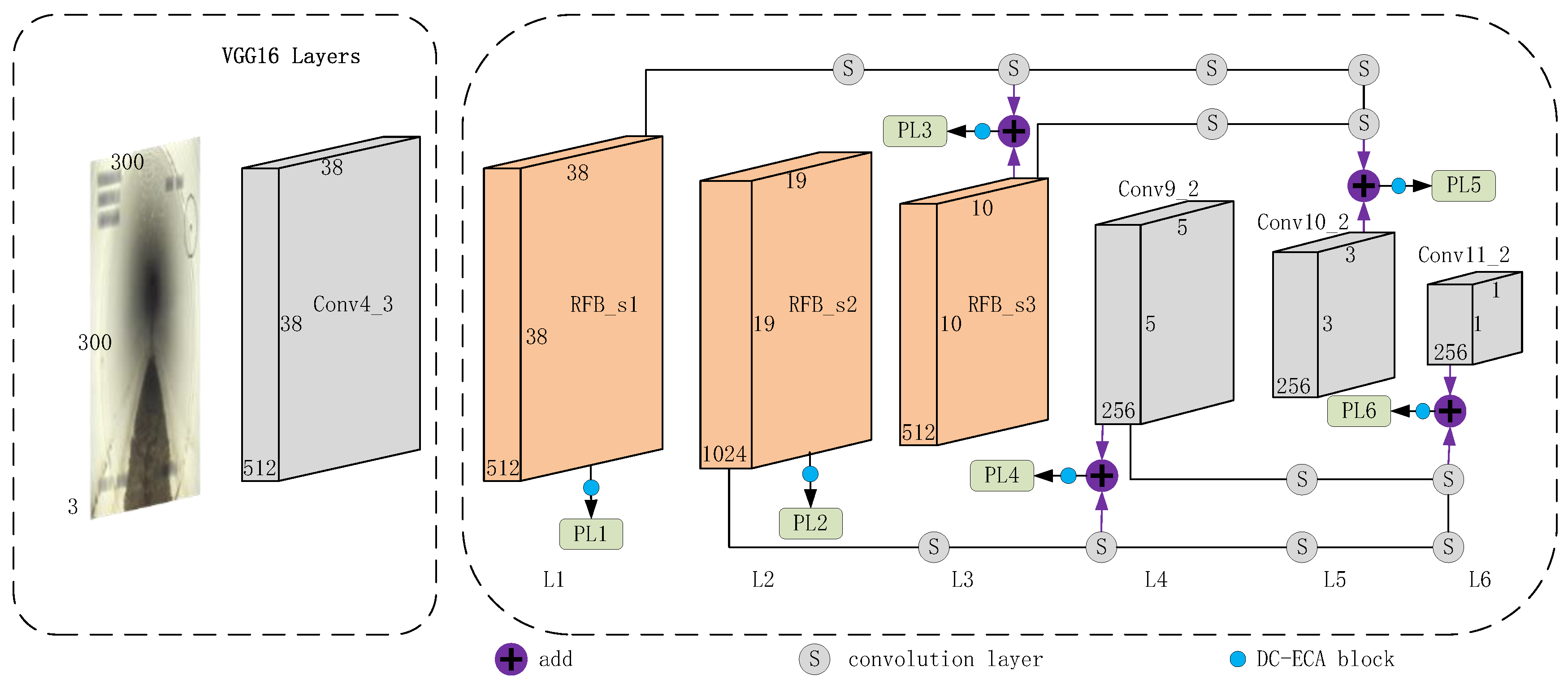
This paper proposes an improved object detection algorithm based on the original SSD. Firstly, to address the diverse forms and sizes of drainage pipeline defects, an improved RFB module is added to the backbone network of SSD. By utilizing the RFB module, the network’s receptive field and multi-scale feature extraction capabilities are enhanced, enriching the extracted feature information and enabling the network to learn different texture features between defective and non-defective parts. In the step of constructing the prediction layer, SDCM uses skip connections to transfer information on small defects from the bottom to the top layer—thereby enhancing the small object information of the prediction layer. Meanwhile, an improved ECA (Efficient Channel Attention) module is used to adjust the weights of the output prediction layer—enhancing the feature expression of the network’s output layer. Finally, to address the complexity of pipeline defect features, the diversity of the same type of defect form, and the problem of feature similarity between different defects, this paper adopts the Focal Loss improved loss function to strengthen the weight of difficult-to-classify defects during model training, improve the imbalance of positive and negative samples during training of the SSD network, and enhance the network’s recognition accuracy for pipeline defects.

The improved network structure is shown in the following Figure 1:

3.1. RFB Module

The interior background of drainage pipelines is complex, and there may be various types of defects in the pipelines—even within the same category—with different sizes and shapes. There are significant intra-class differences, which places higher demands on the feature extraction ability and detection accuracy of the detection network. Therefore, this paper proposes to add an improved RFB module to the backbone network of the algorithm.

RFB is a module that combines the ideas of Inception and dilated convolutions to improve the feature extraction capability of a network by enhancing the receptive field. It uses parallel convolutional filters of sizes 1 × 1, 3 × 3, and 5 × 5 to obtain multi-scale features and introduces three dilated convolutional layers with dilation rates of 1, 3, and 5 to enlarge the network’s receptive field. Finally, it adds a shortcut connection inspired by the ResNet architecture.

To address the problem of some defects in drainage pipes possibly occupying a relatively large proportion in images, this paper uses the RFB_s module. This module adds an additional dilated convolution branch with a dilation rate of 7, as compared to the RFB module. To reduce the number of parameters, a 1 × 7 convolution layer followed by a 7 × 1 convolution layer is used instead of a 7 × 7 convolution layer, as shown in Figure 2.

3.2. SDCM Module

The background information of drainage pipelines is particularly complex, and small target defects are difficult to detect under complex background conditions [22]. SSD performs poorly in detecting small targets mainly because they contain less information, and when the network deepens, most of this information is lost [23].

To enhance the detection ability of small targets in complex background conditions, a skip densely connected module (SDCM) was used for feature fusion [24]. The detailed structure of the SDCM is shown in Figure 3, where the previous layer is tightly connected to the subsequent layer from L1 to L6. L1 and L2 represent RFB_s1 and RFB_s2, respectively. Several consecutive convolutional layers, Conv(i_j), with a stride of 2 are connected to L(i), where i = 1, 2, 3, 4 and j = i + 1, i + 2, …, 6, and Conv(i_j) has the same scale as L(j).

PL1 and PL2 are derived from L1 and L2, respectively, because their feature maps are relatively large. As the network goes deeper, the details on small defects become less visible, which is not conducive to the detection of small defects. Therefore, new prediction layers PL(i) are generated to replace the original L(i; i = 3, 4, 5, 6) for prediction.

PL3 = Conv1_3⊕L3,

PL4 = Conv2_4⊕L4,

PL5 = Conv1_5⊕Conv3_5⊕L5,

PL6 = Conv2_6⊕Conv4_6⊕L6.

The feature fusion method in the formula is an element-wise sum. In general, there are 6 prediction layers of different scales, including PL1 and PL2—generated by L1 and L2, respectively—as well as PL(i; i = 3, 4, 5, 6), produced by feature fusion.

3.3. Attentional Mechanism Module

The attention mechanism is a common weight adjustment mechanism in neural networks that enables the convolutional neural network to adaptively focus on relevant features [25].

Common attention mechanisms include the channel attention mechanism, spatial attention mechanism, and the combination of both. The SE module (Squeeze-and-Excitation Module) [26] and ECA [27] module are two commonly used channel attention mechanisms. The specific implementation of the SE module is as follows:

①

Perform global average pooling on the input feature map.

②

Perform two fully-connected layers, with fewer neurons in the first layer and the same number of neurons as the input feature map in the second layer.

③

After completing the two fully-connected layers, obtain the weights of each channel in the feature map through the sigmoid function.

④

Multiply the obtained weight values with the original input feature map.

The ECA module can be seen as an improved version of the SE module; it removes the fully connected layer in the SE module and uses 1D convolution to fuse the channel information, followed by an activation function to avoid information loss caused by the dimensionality reduction in the fully connected layer, as shown in Figure 4.

We propose a dual-channel Efficient Channel Attention block (DC-ECA Block) based on the ECA module, as shown in Figure 5. The difference between the DC-ECA Block and the ECA module lies in the pooling layer part. The DC-ECA Block simultaneously uses global maximum pooling and global average pooling. The maximum pooling can better preserve the local features of the drainage pipeline, while the average pooling can better preserve the overall features of the pipeline. Therefore, the parallel connection of the two different pooling methods can obtain richer channel features. The input H×W×C features are separately compressed by global max pooling and global average pooling to obtain two 1 × 1 × C feature maps. Then, channel feature learning is performed through 1 × 1 convolution. Finally, the two weight vectors obtained are added, and the final channel weight vector is obtained through the Sigmoid activation function.

We have incorporated DC-ECA blocks into all 6 output feature layers to suppress ineffective features and improve detection accuracy.

3.4. Focal Loss

For one-stage object detection algorithms, the network contains a large number of prior boxes as the input image is processed for feature extraction, and each feature point in the feature layer generates several prior boxes, resulting in a large number of prior boxes in the network. The algorithm used in this paper contains a total of 11,820 prior boxes—of which only a few may be positive samples containing real objects—while others are negative samples, leading to a severe imbalance between positive and negative samples during training. To address this issue, the SSD network controls the positive-to-negative sample ratio at 1:3, which has a certain effect, but is limited. Focal Loss proposes using a weight-based approach to balance positive and negative samples, combining two methods to achieve balance: controlling the weight of positive and negative sample losses and controlling the weight of easy-to-classify and hard-to-classify samples. Therefore, Focal Loss can be used to replace the classification loss in the original loss function.

Controlling the weights of positive and negative sample losses:

The following is the most commonly used cross-entropy loss, taking binary classification as an example:

$$CE(p,y)=\left\{\begin{array}{ll}-\log (p)& \mathrm{if}y=1\\ 1-p& \mathrm{otherwise}\end{array}\right.$$

(1)

$y$ represents the actual label and $p$ represents the predicted value. The cross-entropy loss can be simplified using the following p_t:

$$p_t=\left\{\begin{array}{l}p\hspace{1em}\hspace{1em}\mathrm{if}y=1\\ 1-p\hspace{1em}\mathrm{otherwise}\end{array}\right.$$

(2)

Now:

$$CE(p,y)=CE(p_t)=-\log (p_t)$$

(3)

To mitigate the impact of imbalanced positive and negative samples, we can add a coefficient. When label = 1, ${\alpha }_t=\alpha$; when label = otherwise, ${\alpha }_t=1-\alpha$. The range of α is from 0 to 1.

$$CE(p_t)=-{\alpha }_t\log (p_t)$$

(4)

$${\alpha }_t=\left\{\begin{array}{l}\alpha \hspace{1em}\hspace{1em}\mathrm{if}y=1\\ 1-\alpha \hspace{1em}\mathrm{otherwise}\end{array}\right.$$

(5)

$$CE(p,y,\alpha )=\left\{\begin{array}{l}-\log (p)\ast \alpha \hspace{1em}\hspace{1em}\hspace{1em}\mathrm{if}y=1\\ -\log (1-p)\ast (1-\alpha )\mathrm{if}y=0\end{array}\right.$$

(6)

When the value of $\alpha$ is from 0 to 0.5, the weight of the positive sample loss can be reduced, and the weight of the negative sample loss can be increased; when the value of $\alpha$ is from 0.5 to 1, the weight of the positive sample loss can be increased, and the weight of the negative sample loss can be reduced.

Controlling the weights of easy and difficult-to-classify samples:

In classification tasks, the larger the predicted probability value $p_t$ that a sample belongs to a certain class, the easier it is to classify. Therefore, using $1-p_t$, we can calculate whether it belongs to the easy or hard classification. The specific implementation is as follows:

$$\mathrm{FL}(p_t)=-{(1-p_t)}^{\gamma }\log (p_t)$$

(7)

The modulation coefficient ${(1-p_t)}^{\gamma }$ is used to determine whether a sample is easy or hard to classify in the classification task. The specific implementation method is as follows: when γ = 0, the focal loss is equivalent to the standard cross-entropy function. When γ > 0—as the value of $(1-p_t)$ is between 0 and 1—as $p_t$ tends to 0, the modulation coefficient tends to 1, which contributes significantly to the total loss. As $p_t$ tends to 1, the modulation coefficient tends to 0, which means it contributes very little to the total loss.

Assuming there are two samples with y = 1, and that their classification confidences are 0.9 and 0.6, respectively, if we take γ = 2 and calculate their losses according to the formula, the resulting losses are denoted as $-(0.1{)}^2\log (0.9)$ and $-(0.4{)}^2\log (0.6)$, respectively. If we divide their weights: $\frac{0.16}{0.01}=16$, we can see that the loss of the sample with a classification confidence of 0.6 is greatly increased, and the loss of the sample with a classification confidence of 0.9 is greatly suppressed—thus making the loss function more sensitive to the losses of difficult samples.

The following formulas can be used to control the weights of positive and negative samples, as well as to control the weights of difficult and easy-to-classify samples:

$$\mathrm{FL}(p_t)=-{\alpha }_t{(1-p_t)}^{\gamma }\log (p_t)$$

(8)

4. Experiment and Results Analysis

4.1. Dataset Processing and Evaluation Metrics

There is currently no publicly available dataset for drainage pipe detection in China, and the data recorded by detection companies during each detection task contains relatively few defects. If the training of a network is based on these limited defect data, the dataset may not be sufficient. Moreover, these datasets may have the problem of having a too-uniform shape for the same type of defect, resulting in insufficient training of the network model. Even if the experimental results obtained are relatively good, the model’s robustness will be relatively poor, and it will not be able to adapt to the needs of actual detection work.

We utilized the Sewer-ML public dataset of sewer pipe defects proposed by Joakim Bruslund Haurum and selected 4000 images of the most common defects, including Settled deposits (AF), Displaced joints (FS), Deformations (DE), and Roots (RO) for model training. The ratio of images used for training, validation, and testing was set to 8:1:1. Different data annotation standards can also affect the model’s detection accuracy. As each defect has multiple forms and the background inside the pipe is particularly complex, it is necessary to establish uniform standards for annotating the dataset; otherwise, false detections are likely to occur.

When annotating the dataset, we tried to treat all defects belonging to the same category in a single image as a whole, such as settled deposits and displaced joints, unless there were obvious boundaries or significant distances between the defects.

Evaluation metrics: We adopted mean average precision (mAP) as the evaluation metric in this study. mAP is the average precision (AP) across all categories of network detection, which is used to evaluate the model’s detection accuracy. A predicted result is considered correct if the intersection over union (IOU) between the predicted box and the ground truth box is greater than 0.5.

4.2. Optimal Weight Coefficients

We conducted experiments to find the optimal weighting coefficient for the parameter γ, which controls the weight of difficult-to-classify samples in focal loss. The value of γ ranged from one to five with a step size of one. The value of another parameter α was set to 0.25.

The experimental results are shown in

Table 1. Experimental results of weight coefficient based on EFE-SSD + focal loss.

γ	mAP/%
1	90.32
2	91.95
3	92.20
4	91.75
5	90.37

. Although the commonly used value of γ in focal loss is two, the experimental results indicate that a value of γ = 3 shows better performance on the dataset used in this paper, improving the detection accuracy of the algorithm.

4.3. Comparative Experiment of Mainstream Detection Networks

The performance of our proposed network was compared with some classic object detection algorithms and other methods mentioned in other papers on the dataset, and no additional data augmentation was used for any network.

As shown in Table 1, our proposed network achieved an average precision of 92.2% by adjusting the input image resolution to 300 × 300 pixels and inputting it into the feature extraction network; this was a 2.26% improvement compared to the initial SSD network, and our network had better detection performance than other methods in this paper.

Figure 6 displays the P-R curves of different methods on various types of sewer defects. It can be observed that the proposed method in this paper performs significantly better than other methods in detecting the deformation and displacement of sewer pipes. It also exhibits good performance in detecting settled deposits and root intrusion.

To demonstrate the effectiveness of our method in detecting defects in underground drainage pipes, we compared the detection results of the top four models with the best performance, as shown in

Table 2. Accuracy comparison between EFE-SSD and other detection algorithms.

Methods	Backbone	Input Size	AP/%				mAP/%
			AF	DE	FS	RO
Faster RCNN	Resnet50	600 × 600	94.66	82.07	85.32	85.94	87
RetinaNet	Resnet50	600 × 600	97.33	85.42	89.67	85.81	89.56
YOLO3 [28]	DarkNet	416 × 416	90.64	54.11	81.07	72.19	74.5
YOLO5X	CSPdarknet	640 × 640	97.20	82.58	87.42	94.23	90.36
CenterNet [29]	resnet50	512 × 512	90.75	42.64	60.02	74.58	67
SSD	VGG16	300 × 300	95.65	85.07	92.10	86.96	89.94
Gaussian YOLOv4 [11]	CSPdarknet	416 × 416	93.24	57.47	80.94	77.56	77.3
Qian Xie [12]	VGG16	300 × 300	96.47	82.11	88.09	74.54	85.3
RFB Net	VGG16	300 × 300	98.41	87.37	91.40	86.78	90.1
EFE-SSD	VGG16	300 × 300	96.00	89.43	84.87	88.46	92.2

. We randomly selected drainage pipe images containing different types of defects and evaluated their detection performance, as depicted in Figure 7. In Figure 7e, the manually defined positions and extents of the defects are displayed, while the other rows show the detection boxes predicted by different detection models (different types of defects are color-coded, with green representing Displaced joints, red representing Settled deposits, blue representing Roots, and yellow representing Deformations). By comparing the prediction results of the different models, it is evident that our model’s predictions were closest to the ground truth labels. Our model exhibited superior detection performance compared to other detection models—effectively identifying both scattered Displaced joints and subtle pipe deformations that are challenging to recognize.

Figure 8 represents the confusion matrix of the defect recognition results on sewer pipelines using EFE-SSD. It is evident that there are a significant number of errors in terms of missed detections, where the presence of defects was not identified. This is mainly due to the subtle nature of defects in many areas, making it challenging for the neural network model to accurately recognize them. Consequently, this is the primary reason why the overall accuracy of the improved model did not show substantial improvement. However, from a practical perspective, mild defects have a minimal impact on the functionality of the pipelines.

4.4. Ablation Experiment

As our algorithm consists of several improved components added to SSD, we have verified the effectiveness of the different improvement components on the algorithm’s final performance.

Table 3. Ablation experiment. The checkmark (√) in the table indicates that the module is added to the network.

mAP/%	RFB_s	SDCM	Focal Loss
89.94
90.74	√
91.11	√	√
92.20	√	√	√

shows the effectiveness of the different improvements on the final performance of the SSD-based algorithm. To validate the effectiveness of the RFB_s module added to the original SSD backbone network, we conducted two experiments, as shown in the first two rows of Table 3. The improved network achieved a 0.8% increase in detection accuracy, indicating that increasing the receptive field of the feature layers has a positive effect on obtaining more effective feature information.

The third row of Table 3 shows the result of incorporating SDCM to fuse feature information in the network. The detection accuracy was further improved by 0.37%. The reason for this not-so-obvious improvement in accuracy may be that the dataset contains fewer small defects and more larger ones. However, small defects are also important, because detecting them in a timely manner and repairing them will prevent more serious problems in the future and make repairs easier.

In the fourth row of Table 3, Focal Loss was further added to the loss function, resulting in a 1.09% improvement in mAP. The pipeline background is complex, and there are many difficult-to-classify samples—especially for some defects such as sediment obstructions and tree root invasions, which have similar inter-class samples. The Focal Loss function helped to improve the classification performance for difficult-to-classify defects.

The network we ultimately obtained achieved a mAP of 92.2%, which showed a significant improvement in detection accuracy compared to the original SSD network, and also achieved better detection accuracy compared to other mainstream networks.

5. Conclusions

In order to address the problems of high labor costs and low detection efficiency in the inspection of urban underground drainage pipelines, and to make pipeline defect detection more intelligent, we have designed an improved algorithm based on the SSD network. Compared with traditional single-stage object detection algorithms, the EFE-SSD improves the SSD network by adding RFB_s modules to the backbone network, enhancing the feature extraction ability for images with larger defect areas in the pipeline, and improving the network’s ability to recognize pipeline defects. It also integrates multi-scale features and inherits the feature extraction ability of the SSD network, which improves the detection performance of small target defects to some extent. Moreover, the ECA attention mechanism is used to adjust the channel weights of the output layer and suppress invalid features. Finally, Focal Loss is used to replace the cross-entropy loss in the SSD network, which effectively solves the problem of class imbalance in the training process, increases the weight of difficult-to-classify samples during network training, and enhances the detection ability of the network for drainage pipeline defects—further improving the detection accuracy of the network. Experimental results show that the EFE-SSD is significantly better than other mainstream object detection networks in the detection of drainage pipeline defects.

However, there are still some shortcomings in our proposed algorithm—mainly due to the complexity and large number of parameters of the network, which inevitably leads to slower detection speed compared to other single-stage object detection networks. Nevertheless, given the current situation where detection companies still rely on the manual observation of video recordings to search for defects, there is an urgent need for an intelligent method to replace the existing manual defect searching method. Considering the special nature of drainage pipeline defect detection, our algorithm can achieve higher detection accuracy and better meet practical needs.

References

1. Xiao, Q.; Wang, J.; Chen, H.; Ye, S.; Xiang, L. The detection and evaluation by CCTV and rehabilitation analysis of sewer pipeline in an area of Shenzhen City. Water Wastewater Eng. 2019, 45, 109–114. [Google Scholar]
2. Gao, Y.; Wang, H.; Zhang, S.; Ma, L. Current research progress in combined sewer sediments and their models. China Water Wastewater 2010, 26, 15–27. [Google Scholar]
3. Tan, H.; Lei, J.; Chen, Y.; Hao, J.; Liu, J.; Zhang, A.; Zhang, Y. Investigation and rectification strategy of drainage pipe network in a development zone. Cities Towns Constr. Guangxi 2009, 46, 71–73. [Google Scholar]
4. Zhang, C. Strengthen the planning and construction management of urban drainage pipe networks and ensure their efficient and safe operation. Water Wastewater Eng. 2016, 52, 1–3. [Google Scholar]
5. Kumar, S.S.; Abraham, D.M.; Jahanshahi, M.R.; Iseley, T.; Starr, J. Automated defect classification in sewer closed circuit television inspections using deep convolutional neural networks. Autom. Constr. 2018, 91, 273–283. [Google Scholar] [CrossRef]
6. Li, S.A.; Li, T.; Wen, H.F.; Tao, H.Z. Analysis of CCTV detection results of drainage pipes in a city in South China. Urban Geotech. Investig. Surv. 2022, 5, 169–172+180. [Google Scholar]
7. Cao, J.; Li, Y.; Sun, H.; Xie, J.; Huang, K.; Pang, Y. A survey on deep learning based visual object detection. J. Image Graph. 2022, 27, 1697–1722. [Google Scholar]
8. Lü, B.; Liu, Y.; Ye, S.; Yan, Z. Convolutional-neural-network-based sewer defect detection in videos captured by CCTV. Bull. Surv. Mapp. 2019, 11, 103–108. [Google Scholar]
9. Haurum, J.B.; Moeslund, T.B. Sewer-ML: A multi-label sewer defect classification dataset and benchmark. In Proceedings of the IEEE/CVF Conference on Computer Vision and Pattern Recognition, Nashville, TN, USA, 20–25 June 2021; pp. 13456–13467. [Google Scholar]
10. Yin, X.; Chen, Y.; Bouferguene, A.; Zaman, H.; Al-Hussein, M.; Kurach, L. A deep learning-based framework for an automated defect detection system for sewer pipes. Autom. Constr. 2020, 109, 102967. [Google Scholar] [CrossRef]
11. Ye, S.; Teng, Y.; Wang, Z. Research on Defect Detection of Drainage Pipeline Based on Gaussian YOLOv4. Software 2021, 42, 4. [Google Scholar]
12. Li, D.; Xie, Q.; Yu, Z.; Wu, Q.; Zhou, J.; Wang, J. Sewer pipe defect detection via deep learning with local and global feature fusion. Autom. Constr. 2021, 129, 103823. [Google Scholar] [CrossRef]
13. Wang, J.L.; Deng, Y.L.; Li, Y.; Zhang, X. A Review on Detection and Defect Identification of Drainage Pipeline. Sci. Technol. Eng. 2020, 33, 13520–13528. [Google Scholar]
14. Cheng, J.C.; Wang, M. Automated detection of sewer pipe defects in closed-circuit television images using deep learning techniques. Autom. Constr. 2018, 95, 155–171. [Google Scholar] [CrossRef]
15. Liu, W.; Anguelov, D.; Erhan, D.; Szegedy, C.; Reed, S.; Fu, C.Y.; Berg, A.C. SSD: Single Shot Multibox Detector. In Proceedings of the Computer Vision—ECCV 2016: 14th European Conference, Amsterdam, The Netherlands, 11–14 October 2016. [Google Scholar]
16. Liu, S.; Huang, D. Receptive field block net for accurate and fast object detection. In Proceedings of the European conference on Computer Vision (ECCV), Munich, Germany, 8–14 September 2018. [Google Scholar]
17. Huang, G.; Liu, Z.; Van Der Maaten, L.; Weinberger, K.Q. Densely connected convolutional networks. In Proceedings of the IEEE Conference on Computer Vision and Pattern Recognition, Honolulu, HI, USA, 21–26 July 2017. [Google Scholar]
18. Lin, T.Y.; Goyal, P.; Girshick, R.; He, K.; Dollár, P. Focal loss for dense object detection. In Proceedings of the IEEE International Conference on Computer Vision, Venice, Italy, 22–29 October 2017. [Google Scholar]
19. Liu, L.; Ouyang, W.; Wang, X.; Fieguth, P.; Chen, J.; Liu, X.; Pietikäinen, M. Deep learning for generic object detection: A survey. Int. J. Comput. Vis. 2020, 128, 261–318. [Google Scholar] [CrossRef] [Green Version]
20. Wang, J.; Zhang, T.; Cheng, Y.; Al-Nabhan, N. Deep Learning for Object Detection: A Survey. Comput. Syst. Sci. Eng. 2021, 38, 165–182. [Google Scholar] [CrossRef]
21. Jiao, L.; Zhang, F.; Liu, F.; Yang, S.; Li, L.; Feng, Z.; Qu, R. A survey of deep learning-based object detection. IEEE Access 2019, 7, 128837–128868. [Google Scholar] [CrossRef]
22. Tong, K.; Wu, Y.; Zhou, F. Recent advances in small object detection based on deep learning: A review. Image Vis. Comput. 2020, 97, 103910. [Google Scholar] [CrossRef]
23. Zheng, P.; Bai, H.Y.; Li, W.; Guo, H.W. Small target detection algorithm in complex background. J. Zhejiang Univ. 2020, 54, 1–8. [Google Scholar]
24. Cui, L.; Jiang, X.; Xu, M.; Li, W.; Lv, P.; Zhou, B. SDDNet: A fast and accurate network for surface defect detection. IEEE Trans. Instrum. Meas. 2021, 70, 1–13. [Google Scholar] [CrossRef]
25. Niu, Z.; Zhong, G.; Yu, H. A review on the attention mechanism of deep learning. Neurocomputing 2021, 452, 48–62. [Google Scholar] [CrossRef]
26. Hu, J.; Shen, L.; Sun, G. Squeeze-and-excitation networks. In Proceedings of the IEEE Conference on Computer Vision and Pattern Recognition, Salt Lake City, UT, USA, 18–23 June 2018; pp. 7132–7141. [Google Scholar]
27. Wang, Q.; Wu, B.; Zhu, P.; Li, P.; Zuo, W.; Hu, Q. Supplementary material for ‘ECA-Net: Efficient channel attention for deep convolutional neural networks’. In Proceedings of the 2020 IEEE/CVF Conference on Computer Vision and Pattern Recognition, Seattle, WA, USA, 14–19 June 2020; pp. 13–19. [Google Scholar]
28. Redmon, J.; Farhadi, A. Yolov3: An incremental improvement. arXiv 2018, arXiv:1804.02767. [Google Scholar]
29. Zhou, X.; Wang, D.; Krähenbühl, P. Objects as points. arXiv 2019, arXiv:1904.07850. [Google Scholar]
Figure 1. The network structure of EFE-SSD.
Sustainability 15 09164 g001
Figure 2. Comparison of RFB and RFB_s: (a) RFB block;(b) RFB_s block.
Sustainability 15 09164 g002
Figure 3. Architecture of SDCM.
Sustainability 15 09164 g003
Figure 4. Diagram of ECA Block.
Sustainability 15 09164 g004
Figure 5. Diagram of DC-ECA Block.
Sustainability 15 09164 g005
Figure 6. P-R curves of various defects detected by different methods.
Sustainability 15 09164 g006
Figure 7. Detection results of different networks: (a) Detection results of RFB Net; (b) Detection results of YOLO5x; (c) Detection results of SSD; (d) Detection results of EFE-SSD; (e) GT.
Sustainability 15 09164 g007aSustainability 15 09164 g007b
Figure 8. Confusion Matrix.
Sustainability 15 09164 g008