A Study of the Relevant Parameters for Converting Water Supply to Small Towns in the Province of Alicante to Systems Powered by Photovoltaic Solar Panels

Abstract

Solar energy is presented as the main alternative to conventional energy sources that often rely on burning fossil fuels. However, one major obstacle to its wider adoption is the limited ability to store the energy produced that can only be generated for a few hours daily. One way to overcome this limitation is using photovoltaic energy to power urban water supply pumps. This allows the energy to be stored as potential energy in regulating reservoirs while also taking advantage of the temporal coincidence between the generation of solar energy and the daily and annual water and energy supply consumption. Given that implementing solar energy in pumping devices involves an enormous investment, the optimal payback period is identified as the key indicator to know which population is one in which this action is more advisable. This work aims to find the key factors influencing the payback period of solar photovoltaic installation in urban water supply networks. To accomplish this goal, this study analyzes all 20 municipalities in the province of Alicante (which consume groundwater) where these systems can be implemented. Furthermore, this study facilitates the identification of variables that influence the decision to install a solar photovoltaic system in an urban water supply. By measuring two or three parameters, it becomes possible to easily determine the economic viability of such an investment in towns supplied with groundwater. Furthermore, these results can be extrapolated to other municipalities with similar features (irradiance, inhabitants, etc.). This study also presents a straightforward formula that supply managers can utilize to calculate the payback period of the installation using readily available data. The main factors that affect the recovery period of a photovoltaic solar installation are the difference in monthly supply consumption between winter and summer months and the average water depth.

1. Introduction

Getting resources as necessary for life as water and energy, inexpensively and sustainably, is one of the greatest challenges facing society [1]. The electricity consumption will increase from 24,310 TWh in 2015 to 48,800 TWh in 2050 if current trends continue [2]. This increase in energy consumption is based on the increase in the world’s population and has negative effects on the environment. Using renewable energies is necessary to reduce carbon dioxide emissions into the atmosphere [3,4]. The energy used for water supply processes accounts for 4% of the total [5], which highlights how important it is to use renewable energy for these processes.

Solar energy is the most promising alternative [6]. Earth receives about 173,000 TW of photovoltaic energy from the Sun, 10,000 times higher than the world’s energy consumption [7]. However, only 3% of the energy consumed on the planet comes from solar energy [8], indicating significant potential for growth. Although low efficiency (15–20%) is one reason for its low use [9,10,11], solar energy is already cost-effective over much of the earth’s surface [12,13,14].

Some approaches selected the Alicante Region [15] as the area with the higher intensity of solar radiation in the Valencian Community. Other approaches identified the impact of latitude when determining the optimal renovation period of the solar photovoltaic installation [16,17].

García-López considered the financial viability of self-consumption projects using photovoltaic installations [18], but also their vulnerability to two basic financial risks: variations in the price of energy and the amount of energy generated. One advantage of using solar energy for pumping is that water consumption is higher when solar energy is available [17]. Higher water consumption occurs during the day (when there is greater solar potential) and during the summer months (when there is greater irradiance at these latitudes). Similarly, managing drinking water distribution networks allows the storage of water (and energy) in elevated reservoirs [19,20]. These characteristics mean that solar energy is the most suitable for supplying electricity to water supply pumping stations.

Solar energy and its use in water networks for drinking water and irrigation are in line with the UN’s Sustainable Development Goals 6, 7, and 11, which demonstrates the importance of this issue and has been studied in this research. However, most of these approaches have been conducted in isolated areas without grid connections [21,22,23,24,25,26] because the electricity grid does not reach all areas in numerous regions and cannot meet the energy demands produced by pumping equipment [27]. Other works focused on diminishing CO₂ emissions [28], purifying water with solar energy [29], optimization of the system required to use solar pumping [30,31], or on the convenience or otherwise of using batteries [32,33].

It is common to find economic profit based on its geographical location [12] or to predict the influence of weather on its implementation in a hybrid system supplied by solar energy and the electricity grid [34]. However, so far, no study has been found that investigates the influence of the unique characteristics of the supply network that will be supplied by these pumping systems. Therefore, the primary aim of this work is to discover the most significant factors to quantify the payback period of a solar photovoltaic installation. To this end, 20 models are used to simulate the hydraulic supply of various municipalities in the province of Alicante.

This study identifies towns with a higher interest in using photovoltaic solar panels for powering pumping systems. It explores the key factors influencing the payback period of the investment, providing insights into their impact. The findings will facilitate an understanding of the factors influencing installing a solar pumping system and the reasons behind their impact. This knowledge will help determine the favorable conditions for the installation, utilizing easily accessible data for supply managers.

This study determines towns with a higher interest in utilizing photovoltaic solar panels for powering pumping systems. It explores the key factors influencing the payback period of the investment, providing insights into their impact. The findings will enable the identification of favorable conditions for the installation of solar pumping systems using easily obtainable data for supply managers.

Identifying the limits that most influence profitability, municipal solar pumping installation will allow an a priori idea of the help of these pumping systems to be acquired. This demands data that can be obtained (water consumption, depths, etc.). However, this study does not include municipal networks supplied by surface water (rivers and springs), as it is impossible to find a representative average of the flows. In the province of Alicante, these types of catchments have a much more variable regime depending on the dry/wet cycles than groundwater.

This research is subject to a limitation because it has only been calculated for the province of Alicante. Therefore, the influence described would only apply to regions sharing a similar latitude angle (38°). These factors will consistently affect amortization periods, regardless of their relative importance. Batteries to store energy are to be avoided. Batteries bring about inefficiencies, cost implications, weight issues, short lifespans, and complexity regarding disposal. As an alternative, energy can be stored using elevated water tanks, which simplifies the system, ensures availability, and maintains efficiency [12].

In this research, the primary aim is to identify the key factors that significantly impact the payback period of an investment in a solar-powered pump. Two formulas based on the data collected are presented to provide a rough estimate of the time required for cost recovery. It is important to note that this study focuses only on municipalities supplied with groundwater. To use the estimation formulas effectively, users need to have access to specific data, such as water depth and monthly consumption. These values are typically known by network managers in most developed countries.

2. Materials and Methods

In municipalities supplied by groundwater, the energy cost of groundwater abstraction accounts for 55% of the total cost of water at the consumer’s tap ( 0.11 €/m³) [35]. In addition, the average energy cost of lifting groundwater to the reservoir in the municipalities of the province of Alicante is around 0.9 kWh/m³ [35].

Using the Spanish electricity mix (published by the CNMC on 16 April 2021) of 0.25 kg CO₂/kWh and considering groundwater extraction for drinking water at 122 hm³/year [35], pumping water for supply in the province of Alicante leads to emissions of 27,450 TCO₂/year. This figure would be reduced by implementing solar pumping in water supplies, helping to curb global warming.

The aim of this study is not to estimate how many pumping stations would be profitable to install solar pumping. Factors such as the increase in the yield of solar panels and rising energy prices expand the number of feasible municipalities for installing solar panels. In addition, many catchments have a payback period of fewer than 10 years, so they could already be installed in many supplies in the province of Alicante.

2.1. Input Data

Factors that have been studied are:

1.

Manometric head variation between June and December. This parameter has been adopted in aquifers (wells) where solar pumping has been installed;

2.

Manometric head variation between May and December. Note that variables 1 and 2 are similar, but consider May or June the months with the highest and lowest (December) solar radiation;

3.

Range of the manometric head;

4.

Ratio of water volume consumed in June and December;

5.

Ratio of water volume consumed in May and December;

6.

Ratio of the maximum and minimum monthly water volume of the year. Because these months are different depending on the municipality;

7.

Hydraulic efficiency;

8.

Tank autonomy (capacity/volume consumed);

9.

Average municipal consumption;

10.

Average manometric head;

11.

Maximum manometric head;

12.

Energy cost per m³ of water.

2.1.1. Water Distribution Network Data

To perform this work, it is necessary to know the actual water and energy consumption in each of the municipalities analyzed. For this purpose, we need a calibrated hydraulic simulation model representing water delivery in every municipality. The hydraulic solver used here is EPAnet [36], the most widely used software in the water sector, although this research can be reproduced in any other hydraulic software. The data corresponding to the hydraulic infrastructures have been gathered from the Hydrologic Cycle Department of the Alicante Provincial Council. To perform this study, it will be necessary for the model the following elements:

○

Aquifer: The aquifer used for water abstraction is modeled as a reservoir, where the reservoir’s height represents the monthly average dynamic aquifer level (m). This level refers to the water height after the system has been lowered due to pump operation. To calculate this average depth, the maximum daily depths of the last five years (which correspond to the dynamic levels) are considered, as stated in [37];

○

Piezometric head of the well. A reservoir is added to the hydraulic model to simulate the effect of the water level on the aquifer;

○

Node downstream of the pump, necessary to include the pipeline from the aquifer to the reservoir supplying the town;

○

Tanks. All features describe the tanks (elevation (m), diameter (m), volume (m³), maximum and minimum levels (m), etc.);

○

Water distribution network. To speed up the simulation, the entire network can be simplified as a consumption node and with the municipal hourly consumption pattern;

○

Characteristic curves of the pumping equipment: The model includes the relationship between flow rate and head (pressure) as well as the relationship between flow rate and efficiency.

These relationships are calculated according to the following expressions:

$$Q_x=Q_n\ast \left(\raisebox{1ex}{$n_X$}\!\left/ \!\raisebox{-1ex}{$n_n$}\right.\right)$$

(1)

$${Hm}_x={Hm}_n\ast {\left(\raisebox{1ex}{$n_X$}\!\left/ \!\raisebox{-1ex}{$n_n$}\right.\right)}^2$$

(2)

$$P_x=P_n\ast {\left(\raisebox{1ex}{$n_X$}\!\left/ \!\raisebox{-1ex}{$n_n$}\right.\right)}^3$$

(3)

where

• $n_n$, $n_X$: Nominal speed y when changing frequency (rpm);
• $Q_n$, $Q_x$: Flow rate at $n_n$ and at $n_X$ (m³/h);
• ${Hm}_n$, ${Hm}_x$: manometric head at $n_n$ and at $n_X$ (m);
• $P_n$, $P_x$: Power at $n_n$ and at $n_X$ (kW).

Pumping strategies. Pumping strategies that start and/or stop the pumping equipment are programmed.

○

Efficiency of a water supply network. This parameter has a direct impact on the variation in volume between June and December. Because leaks remain constant throughout the year, lower consumption leads to reduced injected flow. As a result, the supply network experiences higher pressure, which is directly linked to the volume of leakage. This means that the lower the performance of the supply network (greater leaks), the smaller the difference in volume consumed between June and December.

2.1.2. Data Measured in Every Municipality

We use sensors from “Sistema Provincial de Telemedida y Telecontrol” (SISCON), the Hydrologic Cycle Area of the Alicante Provincial Council. These sensors collect data on municipal consumption (via outlet flow meters) and water depths (using depth sensors).

The variables considered are:

○

Base demand. The base demand corresponds to the average daily consumption for each month. This value results from the daily average of each month in the last five years and assumes that each month analyzed has different consumptions. The annual study results from 12 different models;

○

Daily consumption patterns: the hourly pattern for each hour of the day of the simulated month shall be entered. To calculate the consumption patterns, the average of each hour of the day for each month over the last five years has been used;

○

Water depth. The reservoir elevation in the model represents the aquifer. It is calculated as the average depth of the dynamic levels (depth with the pump running) for each month over the past five years.

In addition, 12 SKU 6450oVMC SPEKTRON320 solar radiation meters have been installed for this project (Figure 1). These stations have collected data since 7 and 19 November 2018, and data are collected every half hour. With these data, the number of peak sunshine hours can be calculated from these irradiance data, and their values range between 7 h and 13 h in December and June.

○

Average hourly solar radiation. This parameter has been calculated hourly. Each model incorporates these daily parameters for calculating the number of hours that pumping can work.

For every municipality, the hydraulic simulation model considers the data gathered from the respective measuring stations. In this way, particular conditions, such as the depth of the aquifer level, are calculated by the flows delivered to the consumers (population). The solar radiation data are incorporated into the model considering the values collected at the nearest irradiation measurement station. In 10 out of 12 municipalities, a solar irradiation measuring station is available (

Table 1. Solar radiation sensors and their coordinates in the ETRS89 system.

Town	UTMX	UTMY	Town	UTMX	UTMY
Redován	681,589	4,223,053	Orba	753,762	4,296,672
Pinoso	668,864	4,257,731	Alfafara	713,061	4,296,925
Aigües	729,290	4,265,542	Cañada	690,935	4,280,706
Villena	677,276	4,270,853	Confrides	737,504	4,285,055
Tárbena	751,781	4,286,809	Sagra	754,387	4,299,526
Benimassot	735,190	4,292,504	Lorcha	732,483	4,301,177

). The choice of interpolating between different stations has been discarded because of the similarity in the measured values across these stations. A PV module efficiency of 17% has been adopted since the efficiency ranges between 15 and 20% [9,10,11].

It is important to note that both the radiation sensors used and the panels of the solar parks planned in this study have a vertical orientation of 0°. Although a greater inclination would produce a greater increase in energy, horizontal panels have been chosen because:

• Space requirements. Wherever possible, the best choice is to install solar panels on the tank’s roof. This will limit the available surface area. The greater the tilt angle, the greater the distance needed to avoid shading;
• Weight of the structure. To make sure a certain angle of inclination, a structure (which adds weight to the tank) is required. This will not always be due to overloading, which can sometimes lead to structural problems in the tank;
• Shading: To prevent voltage drops along the power line, it is recommended to position the solar PV installation near the pumping equipment. Because of the limited available land and sloping terrain in wooded areas or valleys, the wells are typically situated in such areas. Solar panels are often installed near each other to minimize the space required for the photovoltaic installation.

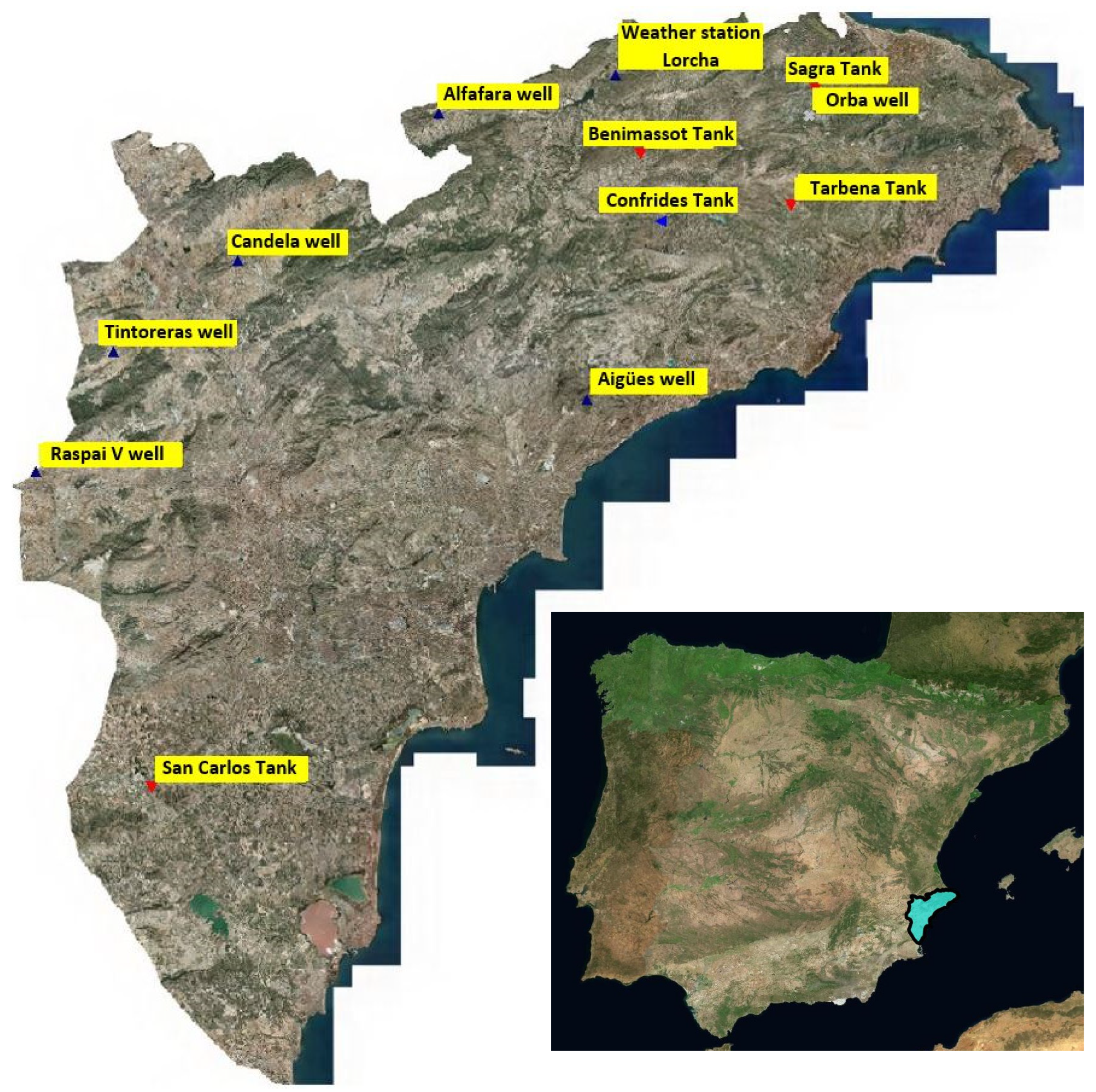
2.1.3. Municipalities Studied

Twenty municipalities in the province of Alicante, in the southeast of Spain, have been analyzed. The primary aim of the research is to find the parameters within the supply networks that have the greatest influence on the payback periods of investments in solar PV installations for powering water-pressurized pumping systems.

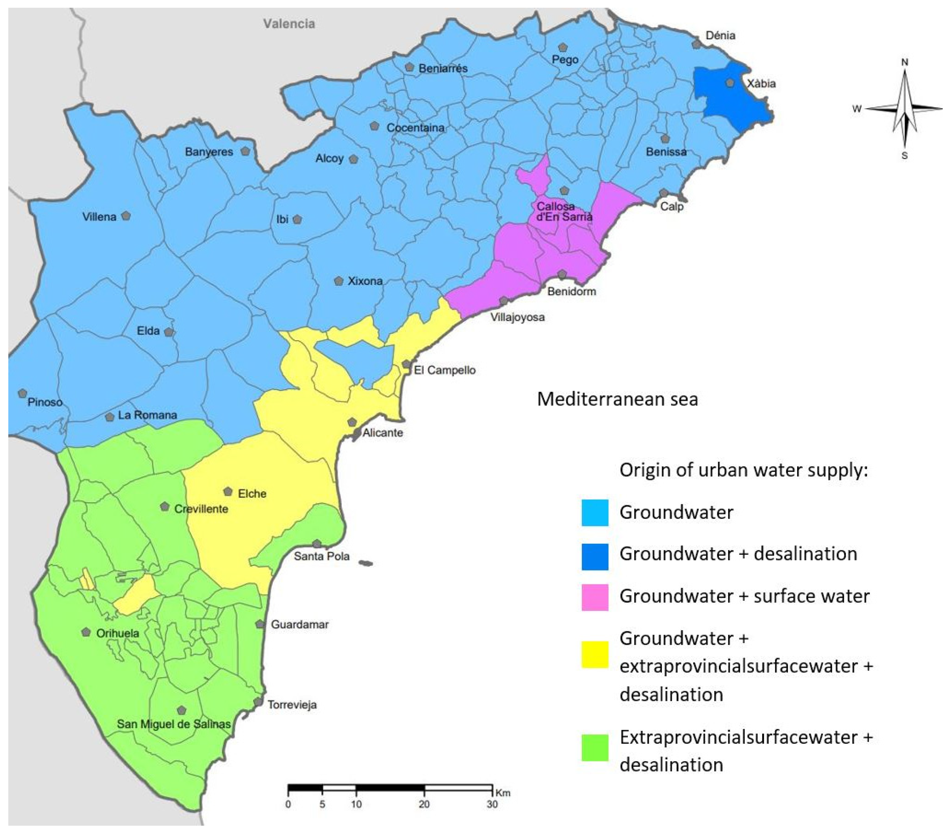
2.1.4. Municipalities Classified According to Drinking Water Origin

Figure 2 classifies the province according to the origin of the water. The entire northern and central area is groundwater, and the town of Xàbia supplied with groundwater and a desalination plant. It can also be seen in the central part of the area around Benidorm, an area (in purple) supplied with surface water and groundwater. The cities of Alicante and Elche (with the largest populations) are supplied by groundwater, desalinated water, and water transfers. In the southern part of the province, the water supply primarily comprises desalinated water and water transfers from other regions and/or hydrological basins (in green). The lower part (in yellow and green) is the only one where water from transfers and desalination appears.

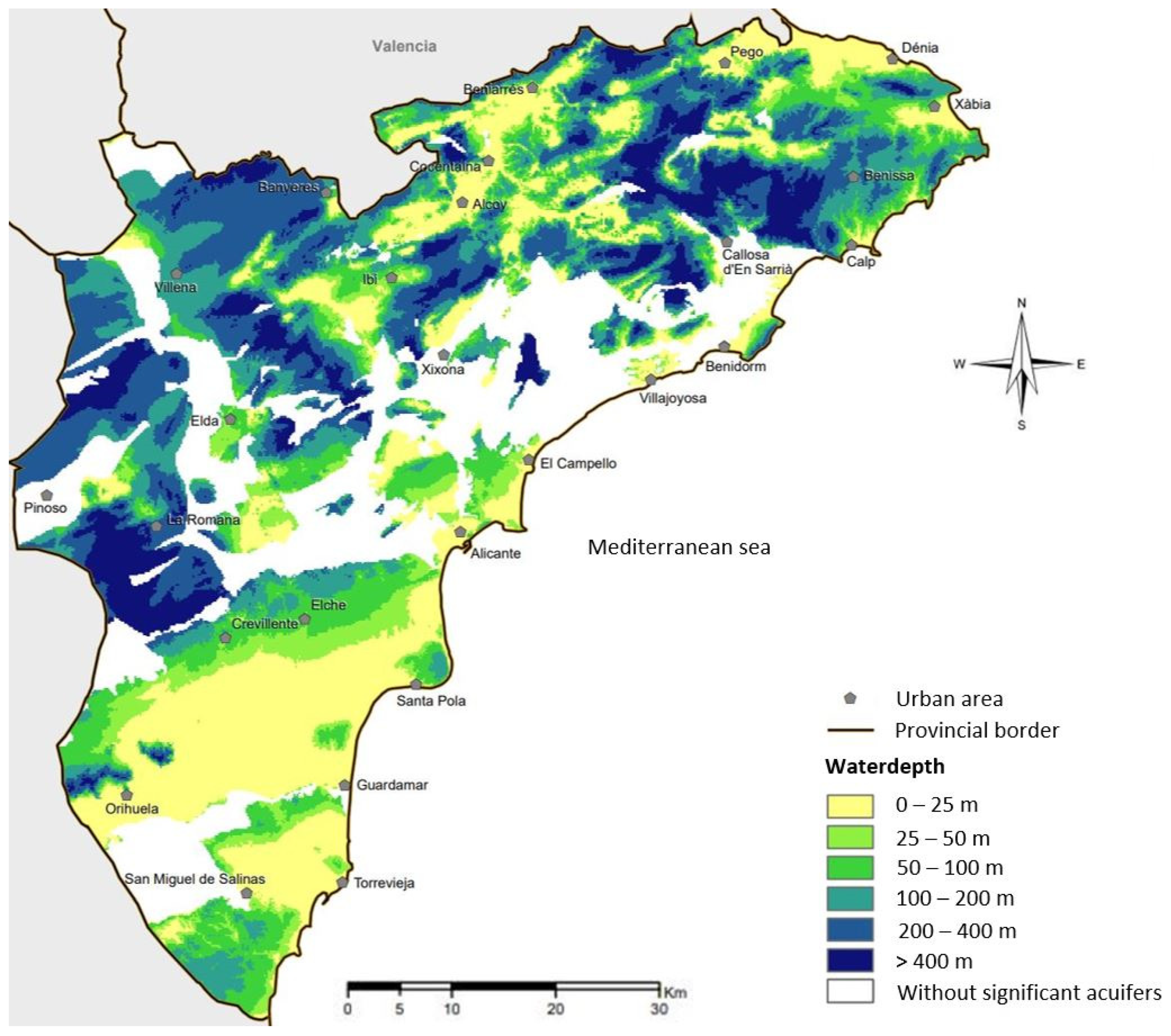
2.1.5. Classification of Municipalities According to the Height at Which Groundwater Is Found

The average water depth in the province of Alicante is known throughout its surface (Figure 3). With this information, if a new water supply borehole is to be built, it will be possible to have an idea of its profitability. The greater the average water depth, the more likely it is that solar pumping is not advisable. Lower average water depths increase the cost-effectiveness of solar pumping.

The greater the average water depth, the more likely it is that solar pumping will not be advisable. As the average depth rises, the energy demand and cost-effectiveness of solar pumping increase.

This estimate can be applied in any area where the aquifer water level is known. The payback period of the installation varies in regions with the same latitude (and the same solar irradiance). To perform this study, over 1600 hydraulic models were simulated based on different municipalities and areas of solar photovoltaic modules. The amortization periods of investments were then compared to certain limits, such as geometric heights (maximum, minimum) or monthly consumption, to establish relationships. Several notable relationships were identified, including the following.

The ratio of water volume consumed in June and December was examined in the study. These months were selected because they represent the highest (June) and lowest (December) solar radiation periods. The findings demonstrate that a greater variation between these consumption levels leads to a shorter payback period. The energy consumed from solar radiation in June is four times higher than in December. In fact, in the municipality where this difference is greatest, June consumption doubles December consumption (the ratio is 1.916).

A larger disparity in demand results in a more aligned annual consumption curve with the annual solar radiation curve. This alignment maximizes solar energy utilization and decreases the investment’s payback period.

2.2. Energy Consumption Calculation

The procedure for simulating each municipality and determining the scenario with the shortest payback period is outlined here.

First, a model of a municipality is adjusted to the characteristics of the 12 months of the year of the supply network. The models represent the current situation (Case 0) with on-grid pumping devices and with a different aquifer depth per month. We develop 12 models for each population.

The operating hours of the pumping equipment are calculated for each month of the study. With the operating hours and the price of electricity (with its hourly discrimination), the economic costs are calculated. These costs are the value to be minimized. The actual electricity bills (obtained from the Alicante Provincial Council) have similar values to those calculated here. However, the real bills are consistently higher due to various factors such as pumping during non-peak hours caused by anomalies such as significant leaks in the supply network, filling of municipal swimming pools, and municipal festivals.

The electricity price used is tariff 3.1aª with hourly discrimination as of May 2019 for all the models carried out. However, this value will not influence the ultimate results, as the aim of this study is the analysis of trends and not the exact amortization periods. It should be noted that the price of energy, and so of the final electricity bill, has risen sharply in Spain since that date. By reducing the amortization periods of the investments examined in this study, the feasibility of installing PV modules for water supply has been enhanced.

The three cases analyzed in this work are described below (Figure 4). The first is the current case (Case 0) with pumping fed from the electricity distribution network. The second (Case 1) is the off-grid case in which the PV modules supply enough electricity to feed pumping stations to deliver water to final consumers in every municipality. Finally, in the hybrid case (Case 2), the electrical supply of the pumping is carried out jointly by the solar panels and the connection to the electrical network when the solar radiation is not enough.

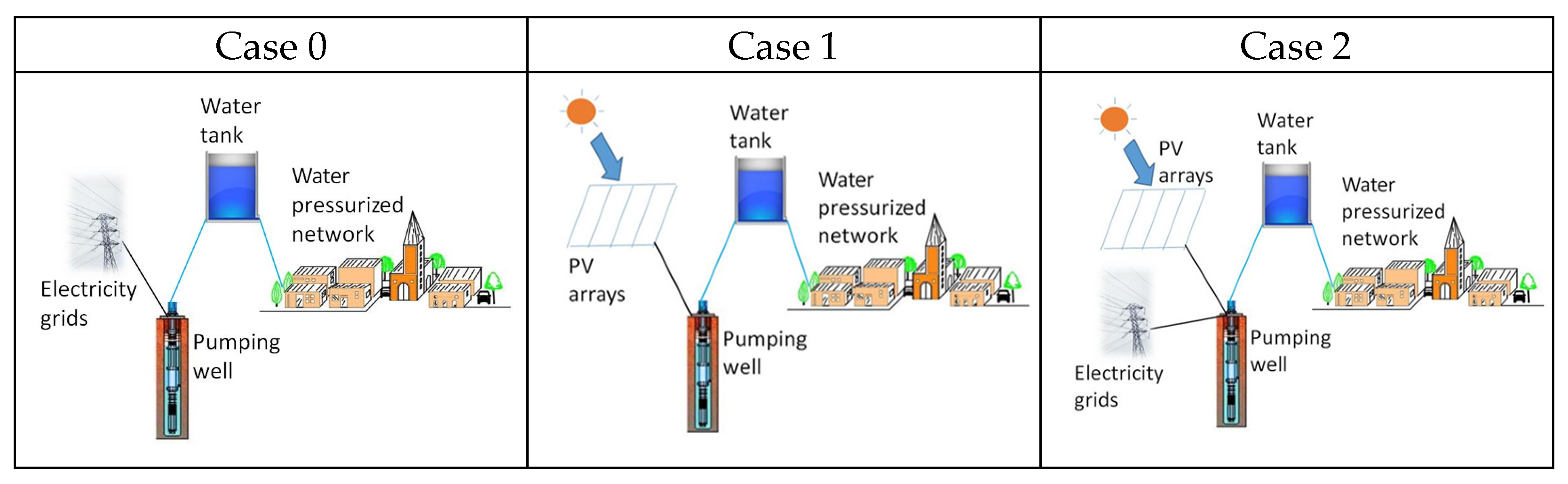
2.2.1. On-Grid Pumping (Case 0)

In case 0, two pumping strategies are considered (for summer and winter). These strategies intend to minimize the pumping hours. The hours in which pumps operate are those with the lowest cost in the electricity tariff.

• A pump is selected with the capacity to pump the daily consumption of the population in 8 h (the number of off-peak hours of the electricity tariff). In most cases, the actual pump in the municipality meets these conditions. The pump must also be able to supply the greatest daily consumption of the year in 24 h, a need to be considered, especially in areas with high seasonality. This restriction was less restrictive than the earlier restriction, and all pumping stations met it;
• The hydraulic problem is solved. The pumps operate during off-peak hours (from 00:00 to 08:00). Peak hours (from 11:00 to 15:00 and from 19:00 to 23:00 in summer and winter) are avoided. The simulation period is equal to 744 h (31-day months); 720 h (30-day months), and 672 h in February (28 days);
• The operating hours are calculated and separated into off-peak, flat, and peak periods. In this way, the cost of the electrical energy consumed each month can be calculated by multiplying the hours by the costs in each period.

The monthly cost is determined by several factors. These include the cost per installed electrical power, the cost of consumed energy, a fixed term for metering equipment rental, and applicable taxes. In these terms, the total cost of the monthly electricity bill is obtained, and the sum of the 12 bills is the annual energy cost.

2.2.2. Off-Grid Pumping (Case 1)

First, we gather the hourly solar radiation averages (in W/m²). With this information, the hours in which the pump has enough energy to work and the highest operating frequency are calculated. For this purpose, the network manager knows the flow-power curve for each operating frequency (data provided by the manufacturer). The start and stop times of the pumps are known.

• We choose the pumping equipment meeting the most unfavorable conditions (December in these latitudes). In situations where oversizing the photovoltaic installation would cause unaffordable investment costs, this condition is not taken into account. For this study, the limit has been set when the amortization period exceeds 30 years.

It is a mandatory condition that the reservoir must have enough capacity to supply the municipality for several days with no inflow of water. This is a strong limitation and means that the investment in increasing the storage capacity is very high [17].

For the present study, this time has been set at five days, considering the solar radiation data used for the calculations.

One condition that must be considered when selecting a pump will be its capacity to pump water at a much higher manometric head than normal operation so that, in this way, when the pump operates at a lower frequency, despite the drop in the pumping curve ${Hm}_x={Hm}_n\ast {\left(\raisebox{1ex}{$n_X$}\!\left/ \!\raisebox{-1ex}{$n_n$}\right.\right)}^2$, it will still have enough manometric heads for the flow to reach the reservoir. However, sometimes this may cause the pump to run at low-efficiency flow rates, which should be avoided.

2.

The hydraulic model is simulated (using a hydraulic solver such as EPAnet) [36]. Here, the pumping conditions will depend on the hours in which enough solar radiation is for the pump to work. If an inverter is available (increasing the cost-effectiveness of solar pumping), the power required at different pump frequencies is calculated to offer more pumping hours.

The hours of pumping operation for each frequency will depend on whether the energy produced by solar radiation suffices to supply the pump with its operating power. For this purpose, the electrical power curves for different frequencies, e.g., 60, 70, 80, and 90%, will be calculated from that already available (100%). In addition, the head and efficiency curves shall also be calculated for the same frequencies.

Once these have been calculated, a pump will be introduced for each frequency (including 100% operation). The pumps will start when they reach their operating power and stop when the pump simulates a higher frequency.

This approach ensures that the pumps only work when there is enough energy generated to operate them at their optimal frequency. Specifically, when the energy generated does not run the pump at 60% of its nominal frequency, the pump will not operate. As the generated energy increases, the pumps will activate one by one in a cascading manner based on their respective frequency requirements. For instance, if the generated energy is between 60% and 70% frequency, the pump set to operate at 60% frequency will work, and so on for other frequency ranges.

3.

The number of pumping hours using solar energy must complete 100% of the water supply to the network; otherwise, the area of the solar park must be increased.

From this point, it can be deduced that the cost of the electricity bill of the well will be €0, so the saving in the bill will be 100%.

4.

The cost of the investment in each scenario and the savings in the electricity bill (obtained by difference with the electricity bill for the case without solar panels) are shown. The point showing the best scenario is in the upper right corner of the graph. It corresponds to the scenario with the highest investment cost and the highest electricity bill savings, due to in this scenario, 100% of the electric bill is saved.

2.2.3. Hybrid Pumping (Case 2)

In Case II, the steps involved will be a combination of those in Cases 0 and I. This means calculating both the electricity bill cost (such as in Case 0) and the solar farm cost (such as in Case I).

Unlike cases 0 and I, where only one scenario was obtained for each municipality/supply network, Case II will yield multiple scenarios corresponding to the number of solar installation sizes to be calculated. In this study, simulations were carried out to identify the optimal point that maximizes savings and investment returns. This point on the graph represents the intersection with the steepest slope when connected with the (0,0) point.

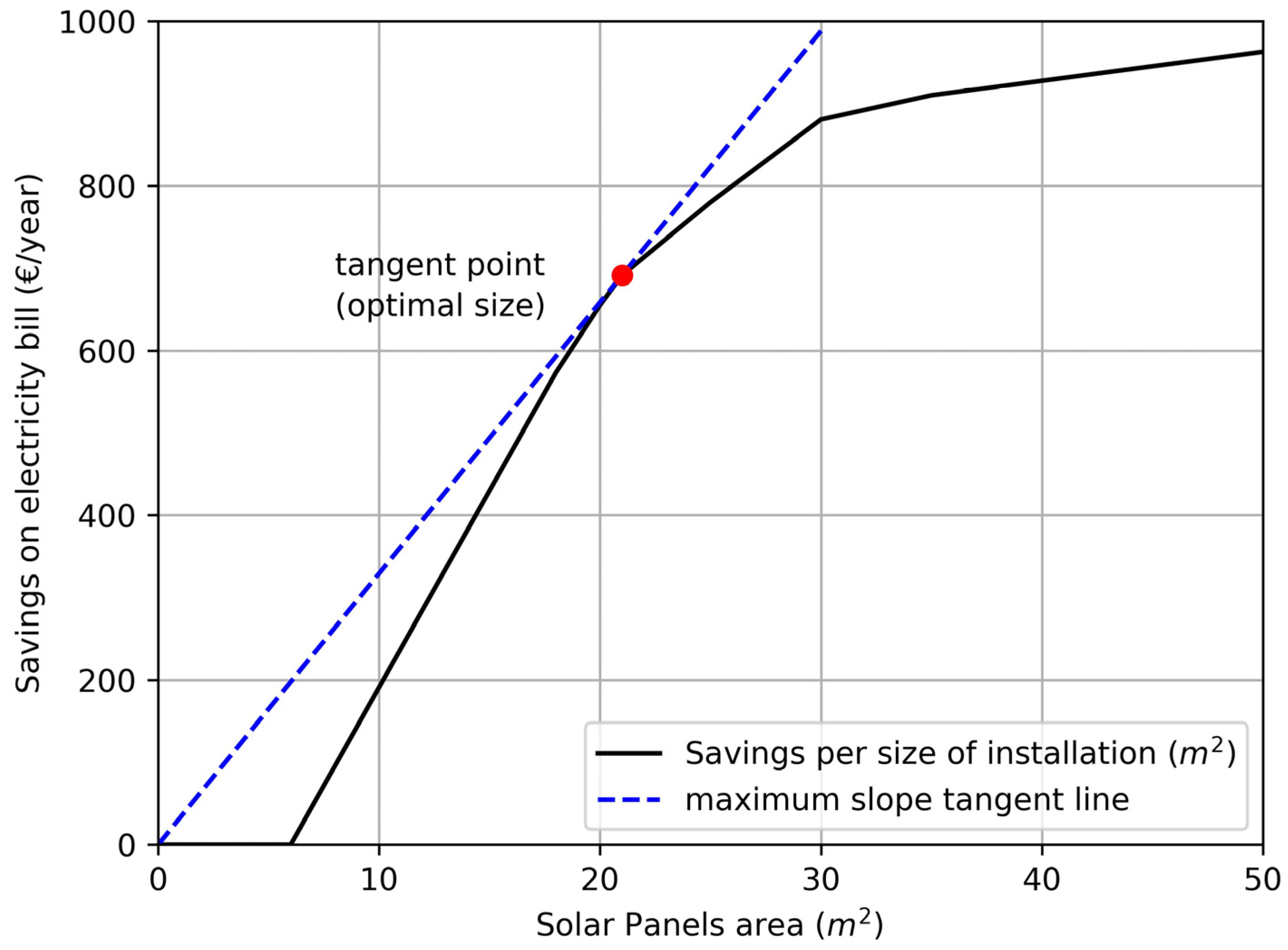
2.2.4. Optimal Point

At least the following points should be shown:

• (0;0) Pumping without solar panels: Corresponds to the conventional scenario (Case 0), in which pumping is conducted with energy from the electricity grid, so neither investment nor savings;
• Largest area of solar PV modules with no savings: This is the scenario in which the dimensions of the solar park are 1 m² smaller than the minimum area in which the solar park would supply the pump with enough power to lift water to the well and, therefore, produce savings in the electricity bill;
• 100% solar pumping (Case I): in this scenario, it will not be necessary to pump using energy from the electricity grid;
• The remaining scenarios necessary for the Savings/Area graph represent the point of least payback period with enough accuracy.

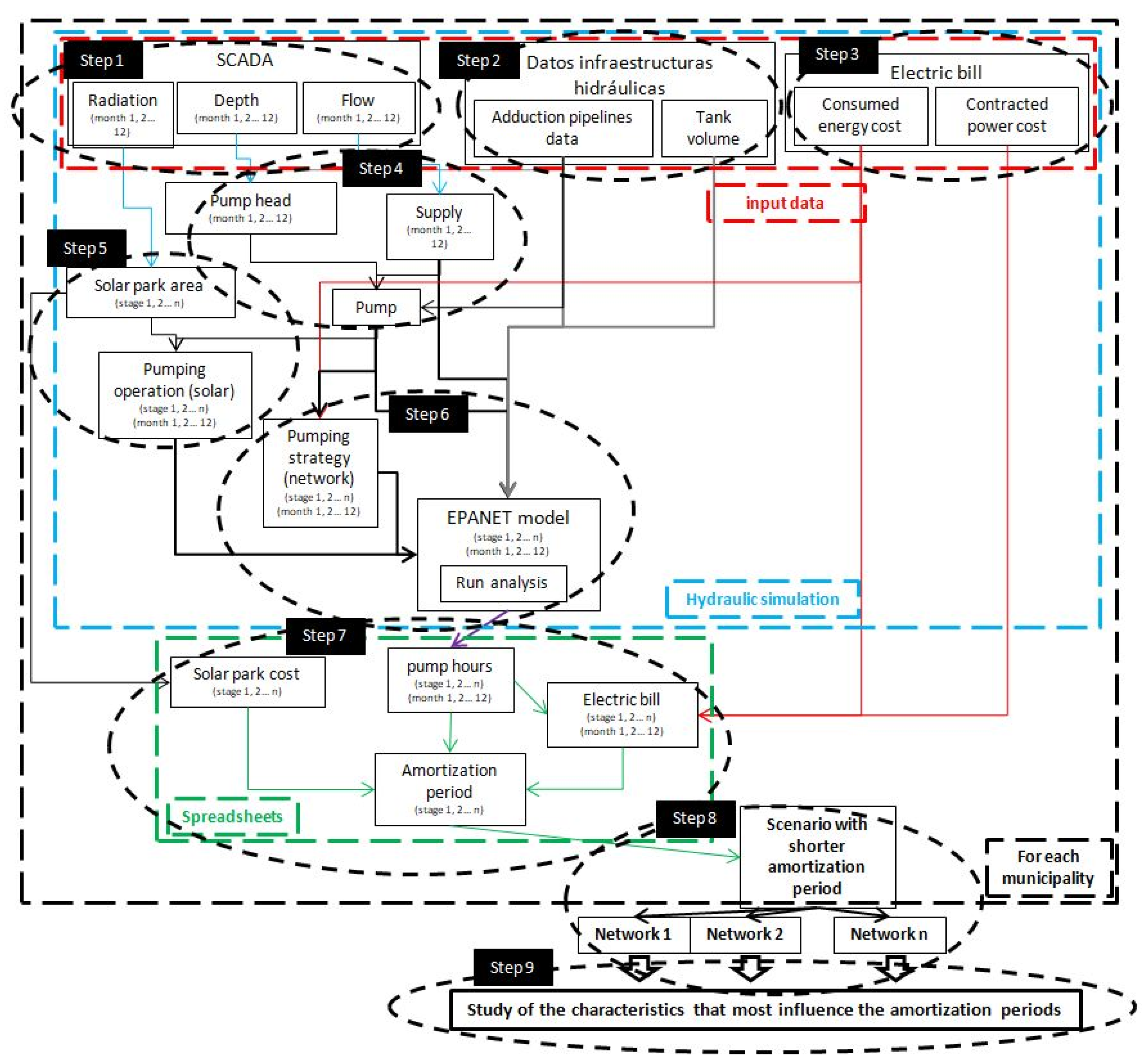
This is also explained in the following section.

2.3. Method

Figure 5 shows the outline of the process followed in this work.

Step 1: Collection of data (radiation, flow, and depth) from the SCADA: First, the data will be organized and cleaned to ensure accuracy and consistency. Any missing or erroneous data points will be corrected or removed. The radiation and flow data have been gathered hourly and exported for the last five years (since the sensors were installed). The greatest daily depth of the aquifer water level is also exported. Once the data are available, they will be treated in the following way:

• Radiation: Daily averages are collected for each month of the year; the ultimate aim is to have the average hourly irradiation for each month;
• Flow: On the one hand, the daily averages are obtained, and the monthly average values are calculated;
• Depth: The average value of the maximum daily depth is collected. These values correspond to the monthly dynamic level and represent the geometric head that the pump needs to overcome. They also account for head losses because of friction. In short, this geometric level difference is the minimum head of the pumping equipment.

Step 2: Data on the municipality’s upstream water infrastructures is collected, including information such as the height of the well and reservoir, reservoir volume, pipe lengths, diameters, roughness, and any special parts that might affect impulsion head losses.

Step 3: Select the electricity tariff to be used in the simulations of cases 0 and II from the possibilities available in the study area.

Step 4: Selecting the pump: the most suitable pump is chosen to consider the reduction in flow rate because of the higher head required (a phenomenon related to the head-flow curve) and the lower head of the pump when operating at lower frequencies. The pump must be able to deliver flow to the tank in the usual frequency range (30–50 Hz) to ensure adequate performance. This need is the most difficult to fulfill and makes the choice of pump difficult.

Step 5: The solar installation will be sized by selecting different areas for each scenario. This process will be repeated until the scenario with the shortest investment payback period is identified. The larger the area of the solar park, the higher the investment cost, but the lower the energy consumed from the grid for pumping, and so, the lower the operating cost. The aim of steps 5, 6, and 7 is to find the point where dividing the investment cost by the annual savings is the lowest, which will show the smallest payback period.

Step 6: Simulation of the eigenfeatures obtained after the first four steps. The new model should represent the chosen to pump strategies.

First, a pump operating with solar energy is considered. For this purpose, the collected irradiation data (step 1), the area of the dimensioned model (step 5), and the efficiency of the solar panels are needed. Because of the calculations, the energy available for solar pumping and the working frequency of the pumps is obtained.

Subsequently, the optimal pumping strategy is selected. This means that necessary simulations are performed to reduce the electricity bill. The energy demand is scheduled when solar modules are producing power. The added hours are reduced to the smallest so that the tank is not emptied, and thus, the water supply is guaranteed. It should also be ensured that these other hours are included in off-peak hours.

Once the complete model has been generated, the hydraulic simulation will be performed to verify that the conditions that the tank has not been emptied or overflowed throughout the month have been met. If this condition is not met, go back to step 6. If so, the results will be exported.

Step 7: The data obtained in the simulations will be exported to a spreadsheet to find the economic cost of pumping according to the Spanish tariff (3.1).

Steps 5, 6, and 7 are repeated for several installations. Different possibilities are dimensioned according to the total areas of the solar panels installed in the solar park. For each case, the investment, the bill savings, and the payback period of the investment are calculated. Figure 6 shows a relation between distinct possibilities, where the X-axis is the investment made and the Y-axis is the savings. The tangent line to the investment vs. savings graph shows that the best is found at the intersection, as future investments lead to lower savings.

The result is a graph showing the cost of the solar installation on the X-axis and the annual savings on the electricity bill on the Y-axis (Figure 6) from the graph generated; the optimal point will be the one that joins the origin (0:0) generate the line with the steepest slope.

Once the optimal investment is known, the payback period is calculated, an indicator against which the different municipalities are compared.

Step 8: List all the characteristics of each municipality that may influence pumping costs. These are the maximum, minimum, and average annual manometric head; maximum, average, and minimum monthly consumption; network efficiency; tank volume, maximum and minimum autonomy of the tank(s); and length of the network and water cost. These parameters are the candidates for influencing the variation between the consumption in June and December and the variation in the pumping head in June and December.

Step 9: Compare the influence of each characteristic of point 8 with the amortization period calculated in step 7 and detect which limits have the greatest influence.

2.4. Relevant Parameters

For each of the municipalities, the following have been chosen as potential representative limits:

• Maximum, minimum, and annual average gauge head;
• Maximum, average, and minimum monthly consumption;
• Efficiency of the supply network;
• Storage volume of the reservoir(s);
• Maximum and minimum autonomy of the tank(s) (depending on seasonal consumptions);
• Length of supply network;
• Cost of water.

Not all of this influences the payback period. Variations between the water consumption in June and December and the variation between the pumping head in June and December are found to be the parameters that best describe the profitability of the investment.

This method can apply to any of the 96 municipalities in the province of Alicante that rely on groundwater abstraction. Additionally, it applies to any water supply that abstracts water from wells, especially in regions with a similar latitude as Alicante.

With higher latitudes, the difference in sunshine hours between June and December has a greater impact. Conversely, near the Equator, this impact is reduced since the hours of sunshine converge to a similar annual value.

The method used includes a Principal Components Study (PCA), which comprises expressing a set of variables as a combination of uncorrelated factors. These factors capture a smaller portion of the overall data variability. By representing the data in a lower-dimensional space, the method minimizes information loss, making it easier to analyze.

PCA differs from factor analysis because it generates uncorrelated factors with commonalities equal to 1 (specific variances are zero).

The principal component analysis is useful for summarizing data on several quantitative variables and acquiring uncorrelated factors. These factors can be used as new variables to avoid multicollinearity in multiple regression or discriminant factor analysis. They can also facilitate automatic classification by retaining only the most essential information, i.e., the first factors.

3. Case Study

As defined in Section 2.1.3, 20 municipalities in the province of Alicante have been analyzed. In the following, the collected irradiation data (Section 3.1) and energy consumption (Section 3.2) are shown. Later, relevant factors are analyzed (Section 3.3), and the payback period is calculated (Section 3.4).

3.1. Monthly Irradiation

Some observe that in 15 of the 20 municipalities, the most favorable month was May, while in the remaining five, it was June. Even though June has higher solar radiation, it also has a higher required volume. In most cases, the increase in water consumption is greater than the increase in solar radiation. In addition, in June, the water depth in the well is greater than in May in all the months studied, which reduces the pumping flow.

December is usually the least favorable month (16 out of 20), and in the remaining cases, November (4 out of 20).

As mentioned in Section 2.1, this study assumes the use of horizontal solar panels. However, if the panels are tilted at a greater angle, the difference in energy produced by solar radiation between June and December decreases. This means that December and January may no longer be the most limiting months. Instead, the most restrictive months could shift to the summer months of May and June. Although in real life, this scenario is never achieved, as the installation would not be optimized.

The shape of irradiance curves exhibits distinct patterns throughout the year and is shown in Figure 7. The characteristics of these curves during the winter months are narrower compared to other seasons, and the province of Alicante has these features during winter months. In regions closer to the equator, less narrowing of the irradiance obtained will be observed. Figure 7 represents the average radiation for each hour of the day for each month of the year. It clearly reflects the difference in energy generated in May, June, and July, where surplus energy occurs, and the clear deficit in November, December, and January.

3.2. Study of Energy Consumption by Month Analyzed

The graph (Figure 8) illustrates how the payback period of a solar pumping system investment decreases as the difference in consumption between December and June increases.

$$C=\frac{Volume consumed in June}{Volume consumed in December}$$

When the pumping head is higher, the delivery flow of a pump decreases because of efficiency losses caused by leakage and turbulence. This means that as the water depth and the elevation height increase, more time is needed to pump the same volume of water. This shows that the availability of water is a crucial factor in determining the size of the photovoltaic system, the cost of investment, and the time to recover the initial investment [38]. Multiplying the above value by the variation between the geometric height in June and December brings the values more in line with the trend line (R² = 0.589; Figure 9). This relationship is not linear. The authors attempted to find other equations to meet the points gathered. Unfortunately, over-fitting problems have appeared, and we prefer to keep an easy formulation to highlight the numbers achieved.

3.3. Principal Components Study

By the principal component analysis, explained in Section 2.3, some observe that despite having a lower R² than the difference between the manometric head in June and December, the difference between the maximum and minimum manometric head of the year has a greater relationship concerning the amortization period of the investment than the previous one (

Table 2. Principal Component Analysis results.

Payback Period. (Years)	Variability	Payback Period. (Years)	Variability
H.m. minimum	0.56	May consumption	0.28
H.m. maximum	0.56	June consumption	0.24
H.m. Average	0.568	December consumption	0.27
H.m. May	0.55	average consumption	0.27
H.m. June	0.53	Cons. June/Cons. December	−0.56
H.m. December	0.53	Storage autonomy (days)	−0.19
H.m. max./H.m. min.	−0.65	June/December	−0.77
H.m. June/H.m. December	−0.53	June/Dec (Hm squared)	−0.71
H.m. May/H.m. December	0.07	June/Dec (consumption squared)	−0.71
H.m. minimum	0.56	H.m. June	0.53
H.m. maximum	0.56	H.m. December	0.53
H.m. Average	0.56	H.m. max./H.m. min.	−0.65
H.m. May	0.54	H.m. June/H.m. December	−0.53
H.m. May/H.m. December	0.07

), so this value has been used together with that of consumption between June and December (chosen for having the greatest relationship between the variables related to the consumption data) to create a formula whose result, introducing only the variables of $\raisebox{1ex}{$.\mathrm{m}.\mathrm{m}\mathrm{a}\mathrm{x}$}\!\left/ \!\raisebox{-1ex}{$\mathrm{H}.\mathrm{m}.\mathrm{m}\mathrm{i}\mathrm{n}$}\right.$. and $\raisebox{1ex}{$\mathrm{C}\mathrm{o}\mathrm{n}\mathrm{s}.\mathrm{J}\mathrm{u}\mathrm{n}\mathrm{e}$}\!\left/ \!\raisebox{-1ex}{$\mathrm{C}\mathrm{o}\mathrm{n}\mathrm{s}.\mathrm{D}\mathrm{e}\mathrm{c}\mathrm{e}\mathrm{m}\mathrm{b}\mathrm{e}\mathrm{r}$}\right.$, of the closest possible value to the amortization period of the investment.

3.4. Calculation of the Amortization Period

The water supply amortization periods range widely, the longest being four times longer than the shortest (

Table 3. Payback periods (in years) for the municipalities.

Town	Payback (Years)	Town	Payback (Years)	Town	Payback (Years)	Town	Payback (Years)
1	7.00	6	17.08	11	20.90	16	23.33
2	12.15	7	17.90	12	21.41	17	25.31
3	12.80	8	19.50	13	21.93	18	25.45
4	13.80	9	20.41	14	23.05	19	27.51
5	15.51	10	20.69	15	23.22	20	27.67

). This shows the heterogeneity in the characteristics of the supply networks, which influence the payback period. This underlines how important it is to know the population to identify investment profitability.

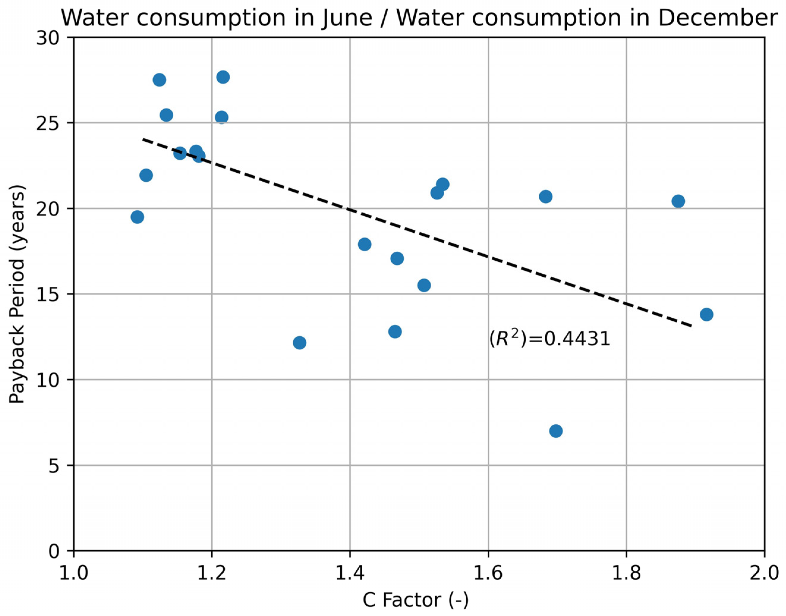
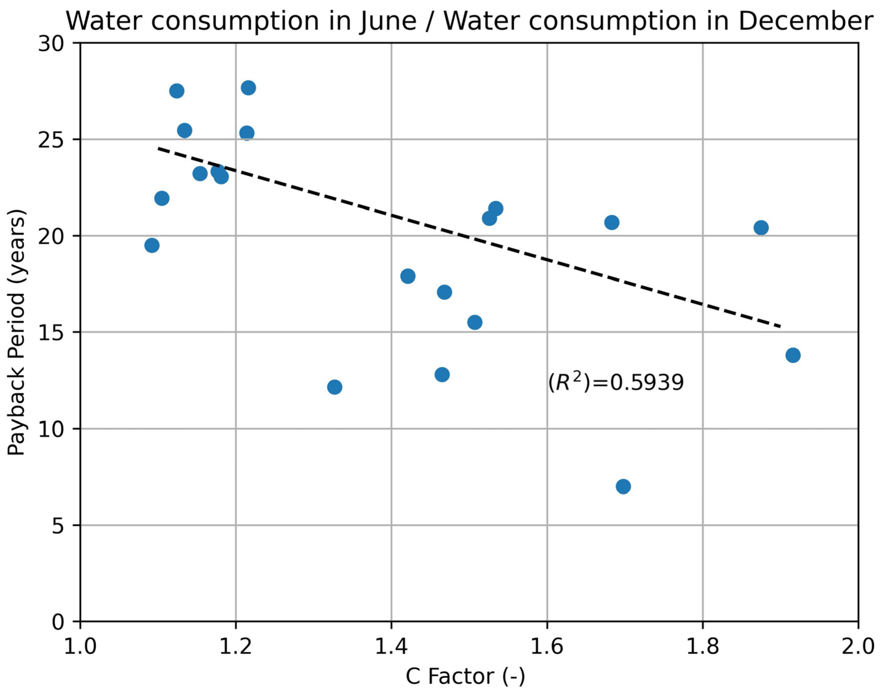
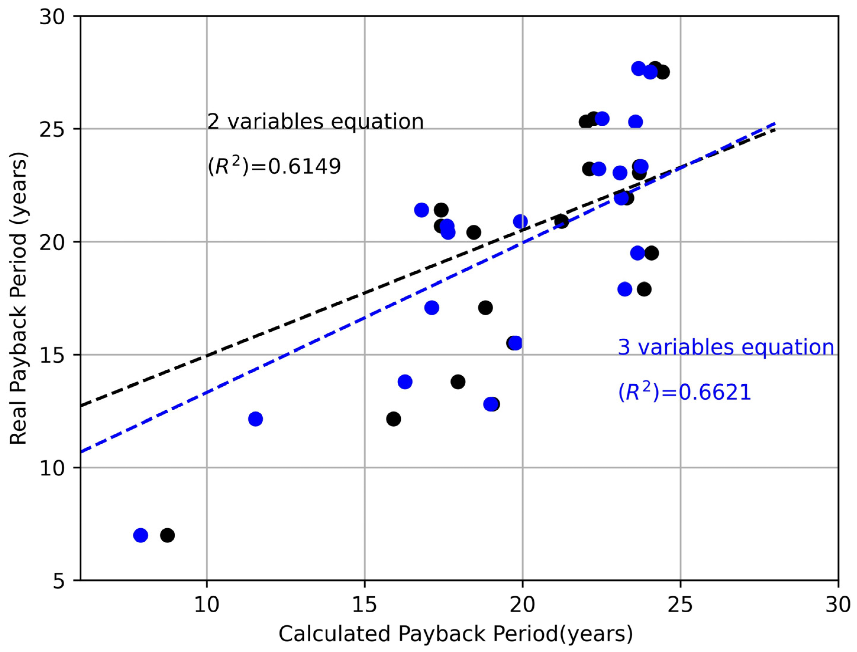
3.5. Adjustment of the Amortization Period from the Representative Variables

A formula calculated the amortization period of the investment considering the most influential parameters. The coefficients must be raised to two exponents and multiplied by each other and a third number. The multiple of these values will be subtracted from a fourth constant, and the result will be the calculated payback period. The structure of the formula, therefore, will be:

$$CAP=C-A\ast {\left(\frac{\mathrm{H}.\mathrm{m}.\mathrm{m}\mathrm{a}\mathrm{x}}{\mathrm{H}.\mathrm{m}.\mathrm{m}\mathrm{i}\mathrm{n}}\right)}^{\alpha }\ast {\left(\frac{\mathrm{C}\mathrm{o}\mathrm{n}\mathrm{s}.\mathrm{J}\mathrm{u}\mathrm{n}\mathrm{e}.}{\mathrm{C}\mathrm{o}\mathrm{n}\mathrm{s}.\mathrm{D}\mathrm{e}\mathrm{c}\mathrm{e}\mathrm{m}\mathrm{b}\mathrm{e}\mathrm{r}}\right)}^{\beta }$$

where

• CAP: Calculated amortization period (years)
• C: Constant (dimensionless)
• A: Multiplier factor (dimensionless)
• α and β: Boosting factors (dimensionless)
• $\frac{\mathrm{H}.\mathrm{m}.\mathrm{m}\mathrm{a}\mathrm{x}}{\mathrm{H}.\mathrm{m}.\mathrm{m}\mathrm{i}\mathrm{n}}$: Maximum manometric head/Minimum manometric head, annual (dimensionless).
• $\frac{\mathrm{C}\mathrm{o}\mathrm{n}\mathrm{s}.\mathrm{J}\mathrm{u}\mathrm{n}\mathrm{e}.}{\mathrm{C}\mathrm{o}\mathrm{n}\mathrm{s}.\mathrm{D}\mathrm{e}\mathrm{c}\mathrm{e}\mathrm{m}\mathrm{b}\mathrm{e}\mathrm{r}}$: Volume consumed in June/Volume consumed in December (dimensionless).

The constant and the study parameters must be subtracted to shorten the amortization periods. The parameters were calculated using the GRG algorithm.

The algorithm changes the parameter values to obtain the best fit. The goodness of fit is quantified with the square of the Pearson correlation coefficient (R²), which is better when closer to unity. With the calculated data, a change is made, obtaining the following results:

$$CAP=64.72-38.27\ast {\left(\frac{\mathrm{H}.\mathrm{m}.\mathrm{m}\mathrm{a}\mathrm{x}}{\mathrm{H}.\mathrm{m}.\mathrm{m}\mathrm{i}\mathrm{n}}\right)}^{0.247}\ast {\left(\frac{\mathrm{C}\mathrm{o}\mathrm{n}\mathrm{s}.\mathrm{J}\mathrm{u}\mathrm{n}\mathrm{e}.}{\mathrm{C}\mathrm{o}\mathrm{n}\mathrm{s}.\mathrm{D}\mathrm{e}\mathrm{c}\mathrm{e}\mathrm{m}\mathrm{b}\mathrm{e}\mathrm{r}}\right)}^{0.286}$$

The similarity of the values of the coefficients α and β show that the parameters ((H.m.max.)/(H.m.min)) and ((Cons.June.)/(Cons.December)) have very similar influences in the period of amortization. To compute the relative error for the payback period formula, we consider the uncertainty associated with measured variables. The measurements of $\mathrm{H}.\mathrm{m}.\mathrm{m}\mathrm{a}\mathrm{x}$, $\mathrm{H}.\mathrm{m}.\mathrm{m}\mathrm{i}\mathrm{n}$ have a relative error of 1% for each parameter, and the $\mathrm{C}\mathrm{o}\mathrm{n}\mathrm{s}.\mathrm{J}\mathrm{u}\mathrm{n}\mathrm{e}.$ And $\mathrm{C}\mathrm{o}\mathrm{n}\mathrm{s}.\mathrm{D}\mathrm{e}\mathrm{c}\mathrm{e}\mathrm{m}\mathrm{b}\mathrm{e}\mathrm{r}$ have a relative error of 2%. Therefore, the CAP value can be obtained by calculating the relative error average deviations. Since $z=x\ast y$, then $\Delta z=\Delta x+\Delta y$, which can be written more compactly by forming the relative error, that is $\frac{\Delta z}{z}=\frac{\Delta x}{x}+\frac{\Delta y}{y}$. The same rule holds for multiplication, division, or combinations.

Therefore, the CAP relative error is equal to $0.99\ast 0.99\ast 0.98\ast 0.98=0.9412=1-X_1$. and $1.01\ast 1.01\ast 1.02\ast 1.02=1.0613=X_2$. Being $X_1=5.87\%$ and $X_2=6.13\%$. In short, the CAP value range among the values $\left[CAP-5.87\%,CAP+6.13\%\right].$

This trend allows having an approximate idea of the amortization period of the investment of the solar power system, knowing data that is very easy to obtain, such as the monthly supply volumes and the geometric height of the impulsion.

This analysis was done with all available variables to get a precise formula, regardless of the number of variables. However, results show that only two of the variables and the June manometric head/December manometric head factor have a significant impact on the amortization period. This gives us the following formula:

$$CAP=C-A\ast {\left(\frac{\mathrm{H}.\mathrm{m}.\mathrm{m}\mathrm{a}\mathrm{x}}{\mathrm{H}.\mathrm{m}.\mathrm{m}\mathrm{i}\mathrm{n}}\right)}^{\alpha }\ast {\left(\frac{\mathrm{C}\mathrm{o}\mathrm{n}\mathrm{s}.\mathrm{J}\mathrm{u}\mathrm{n}\mathrm{e}.}{\mathrm{C}\mathrm{o}\mathrm{n}\mathrm{s}.\mathrm{D}\mathrm{e}\mathrm{c}\mathrm{e}\mathrm{m}\mathrm{b}\mathrm{e}\mathrm{r}}\right)}^{\beta }\ast {\left(\frac{\mathrm{H}.\mathrm{m}.\mathrm{J}\mathrm{u}\mathrm{n}\mathrm{e}}{\mathrm{H}.\mathrm{m}.\mathrm{D}\mathrm{e}\mathrm{c}\mathrm{e}\mathrm{m}\mathrm{b}\mathrm{e}\mathrm{r}}\right)}^{\gamma }$$

where

• CAP: Calculated amortization period (years)
• C: Constant (dimensionless)
• A: Multiplier factor (dimensionless)
• α, β and Υ: Boosting factors (dimensionless)
• ((H.m.max.)/(H.m.min)): Maximum manometric head/Minimum manometric head, annual (dimensionless).
• ((Cons.June.)/(Cons.December)): Volume consumed in June/Volume consumed in December (dimensionless).
• ((H.m.June.)/(H.m.December)): Manometric head for June/Manometric head for December (dimensionless).

Obtaining the following values for the case study:

$$CAP=\mathrm{33,738}-8162\ast {\left(\frac{\mathrm{H}.\mathrm{m}.\mathrm{m}\mathrm{a}\mathrm{x}}{\mathrm{H}.\mathrm{m}.\mathrm{m}\mathrm{i}\mathrm{n}}\right)}^{0.46}\ast {\left(\frac{\mathrm{C}\mathrm{o}\mathrm{n}\mathrm{s}.\mathrm{J}\mathrm{u}\mathrm{n}\mathrm{e}.}{\mathrm{C}\mathrm{o}\mathrm{n}\mathrm{s}.\mathrm{D}\mathrm{e}\mathrm{c}\mathrm{e}\mathrm{m}\mathrm{b}\mathrm{e}\mathrm{r}}\right)}^{1.08}\ast {\left(\frac{\mathrm{H}.\mathrm{m}.\mathrm{J}\mathrm{u}\mathrm{n}\mathrm{e}}{\mathrm{H}.\mathrm{m}.\mathrm{D}\mathrm{e}\mathrm{c}\mathrm{e}\mathrm{m}\mathrm{b}\mathrm{e}\mathrm{r}}\right)}^{0.728}$$

Proceeding analogously here with an equation with three variables, and also considering that the measurements of $\mathrm{H}.\mathrm{m}.\mathrm{J}\mathrm{u}\mathrm{n}\mathrm{e}$, $\mathrm{H}.\mathrm{m}.\mathrm{D}\mathrm{e}\mathrm{c}$ have a relative error of 1% for each parameter, the values calculated are $X_1=8.67\%$ and $X_2=9.33\%$. The CAP value range among the values $\left[CAP-8.667\%,CAP+9.33\%\right]$.

R² increased from 0.6149 to 0.6621 (Figure 10) using the new formula. This action does not demand an increase in the number of necessary data. This is achieved by incorporating a coefficient into the formula, which relates to the previous one ((H.m.June)/(H.m.December)), and can be computed using the average manometric head data for each month. This data are essential for calculating the parameter ((H.m.max.)/(H.m.min)), already used in the previous formula. Considering the significant variations in the characteristics of the municipalities, it is challenging to find a single explanation for such disparities. It is possible that the parameters being analyzed have been simplified or condensed, which could contribute to the observed variations. In this way, it is still necessary to know only the values of the monthly supply volume and the average monthly manometric head of the impulsion to apply the method developed in this study.

3.6. Influence of Piezometric Head Differences

The graphs suggest a large variation should be considered when planning a solar pumping installation. The limit for increased profitability has not been determined, but the difference between the maximum and minimum radiation is around four, suggesting the limit is close to that.

The results obtained allow us to verify the shortest amortization period. The larger these variations are, the more profitable solar pumping is. Figure 11 illustrates the manometric head and water consumption differences between June and December. Green circles signify the five shortest amortization periods, red circles signify the five longest, and black circles the remaining 10. It is observed that the lower values of June volume/December volume and H.m.June/H.m.December, the longer the payback period of the investment will be.

Factors such as solar panel yields, cost, and energy prices affect amortization periods. Implementing solar pumping is becoming more profitable as solar panels become more advanced. Their cost decreases, and the price of energy is suffering a significant increase in recent years.

Factors such as savings and renewal periods are important for determining solar pump profits. The useful life of solar panels is between 25 [17,39] and 30 years [40,41]. Publications corroborate shorter optimal renewal periods, in ranges between 17 and 24.7 years [16]. Trends compared with benefits (at 20, 25, and 30 years) were analyzed to discuss potential trends.

4. Discussion

The uncertainty surrounding the feasibility of installing photovoltaic panels for urban supply pumps often leads to hesitation in making such investments. Therefore, it is crucial to develop a simple and effective method for determining how profitable this investment is. While many studies on solar energy for water pumping have been performed, none have examined the characteristics of water supplies that make the installation more cost-effective.

We discussed key uncertainties related to water consumption and solar irradiance. We analyzed water usage and aquifer water level monthly and daily. For the latter, we measured solar irradiation over the last four years at nine different stations in the northern half of the province of Alicante. The results present a payback period between 7 and 27 years that is similar to those found in line with the 11.10 years found by [17]. Other approaches achieved lower values, such as 6.08 for a municipality in Alicante [42] and also for an installation whose investment will never be covered (the payback period is infinite).

Ensuring 24 h of supply, our study focused on keeping water levels in reservoirs above 1/3 of their total volume. This hindered optimization and raised costs but supplied a guarantee of supply in case of failure.

Our findings showed that December was typically the least favorable month for pumping (16 out of 20) because of rising water levels in the aquifer. This led to a decrease in the manometric head required by the pump and an increase in the flow rate supplied for the same energy consumption. May was found to be the most favorable month for solar pumping (15 out of 20), followed by June (5 out of 20).

We also investigated whether the inertia of the aquifer capacity (i.e., the speed of variation of the water level about rainfall) affected the amortization period of the investment. However, our results showed that it did not have a significant influence. The factors that had a decisive impact on savings were the difference in water depths in the well and the variation in supply volume between the months with the highest and lowest solar radiation.

A difference in depths/consumption between June and December does not guarantee the same difference between the months with the highest and lowest solar radiation.

4.1. Future Developments

This research studies the possibility of using solar pumping to supply municipalities. It can be used to compare characteristics across different areas.

4.2. Recommendation for Practitioners

Solar PV energy is recommended for feeding pumps. Solar energy decreases depending on other energy sources, leading to lower carbon emissions and a positive effect on the environment. Solar PV installations are a sustainable energy option. This reduces dependence on the grid and ensures a continuous water supply, even during power outages or disruptions. Moreover, solar PV systems often require minimal maintenance and have a long lifespan, resulting in cost savings. Solar PV systems for pumps may result in financial savings and government incentives. Solar PV energy is an environmentally friendly and financially sound long-term option.

Several designs have shown potential in harnessing solar energy for pump operations. Among them,

• Incorporating advanced solar panels with high conversion efficiency allows for optimal energy generation even in low-light conditions;
• Innovative storage systems enable efficient utilization of solar energy during non-daylight hours;
• Combination of solar panels and wind turbines, providing a hybrid renewable energy solution for continuous pump operation.

While all these designs exhibit promise, the authors believe the third holds the most potential for a promising future. Combining solar and wind energy reduces dependence on one source and provides energy in varying weather conditions. Furthermore, this hybrid approach maximizes energy efficiency while providing uninterrupted pump operation. The authors expect that this design will gain traction and play a significant role in the future of solar-powered pump systems.

5. Conclusions

Energy plays a critical role in urban supply networks that rely on groundwater, accounting for a significant portion of the total supply cost. The daily pumping of water to the header tank consumes a substantial amount of energy. Therefore, it is crucial to explore energy sources that can reduce this economic burden while minimizing CO₂ emissions. However, the payback periods of investments in such pumping systems vary based on their specific characteristics.

This study seeks to help water supply managers decide where to install solar PV panels for the most economic benefit. This approach seeks to optimize economic outcomes concerning water supply characteristics and limitations. The data analyzed grant valuable insight to organizations granting subsidies. This empowers them to make well-informed decisions based on reliable insights.

Additionally, this study identifies the potential for future research on the feasibility of connecting solar pumping for urban supply to irrigation networks. This connection is possible since the difference in consumption between summer and winter months is significantly higher in irrigation than in human supply. In this way, surplus volumes could be sold during months of high agricultural demand or exchanged for volumes during months with low irrigation demand. This finding opens up new opportunities for exploring innovative solutions that benefit both the urban and agricultural sectors. In fact, the Alicante Provincial Council will take this into account in the coming years when choosing the municipalities in which solar pumps will be installed.

This study’s findings underscore the significance of carefully selecting the supply network for solar pump installations. The amortization periods vary considerably, with the shortest period being almost a quarter of the longest (7 years versus 27.67 years). This highlights the importance of considering supply characteristics to maximize the effectiveness and efficiency of solar pump investments. Practitioners in other regions can adopt the formulas obtained to acquire a quick estimation of the installation payback period.

References

1. Palacios-Cabrera, T.A.; Valdés-Abellán, J.; Jódar-Abellán, A.; Rodrigo-Comino, J. Land-use changes and precipitation cycles to understand hydrodynamic responses in semiarid Mediterranean karstic watersheds. Sci. Total Environ. 2022, 819, 153182. [Google Scholar] [CrossRef] [PubMed]
2. Ram, M.; Bogdanov, D.; Aghahosseini, A.; Gulagi, A.; Oyewo, A.; Child, M.; Caldera, U.; Sadovskaia, K.; Farfan Orozco, F.; Noel, L.; et al. Global Energy System based on 100% Renewable Energy: Energy Transition in Europe Across Power, Heat, Transport and Desalination Sectors. In Study by LUT University and Energy Watch Group; Research Reports 89; Lappeenranta University of Technology: Lappeenranta, Finland, 2018. [Google Scholar] [CrossRef]
3. Kang, J.-N.; Wei, Y.-M.; Liu, L.-C.; Han, R.; Yu, B.-Y.; Wang, J.-W. Energy systems for climate change mitigation: A systematic review. Appl. Energy 2020, 263, 114602. [Google Scholar] [CrossRef]
4. Liu, S.; Yuan, J.; Deng, W.; Luo, M.; Xie, Y.; Liang, Q.; Zou, Y.; He, Z.; Wu, H.; Cao, Y. High-efficiency organic solar cells with low non-radiative recombination loss and low energetic disorder. Nat. Photonics 2020, 14, 300–305. [Google Scholar] [CrossRef]
5. IEA. World Energy Outlook 2019; IEA: Paris, France, 2019. Available online: https://www.iea.org/reports/world-energy-outlook-2019 (accessed on 1 November 2019).
6. Saleh Yassien, H.; Alomar, O.; Mohamed Salih, M. Performance analysis of triple-pass solar air heater system: Effects of adding a net of tubes below absorber surface. Sol. Energy 2020, 207, 813–824. [Google Scholar] [CrossRef]
7. Oishi, A.; Tanjim, M.; Ali, M.T. Loss Analysis of Market Available Solar Cells and Possible Solutions. Int. J. Sci. Eng. Res. 2019, 10, 210–216. [Google Scholar] [CrossRef]
8. Halkos, G.; Gkampoura, E.-C. Reviewing Usage, Potentials, and Limitations of Renewable Energy Sources. Energies 2020, 13, 2906. [Google Scholar] [CrossRef]
9. Sugianto, S. Comparative Analysis of Solar Cell Efficiency between Monocrystalline and Polycrystalline. INTEK J. Penelit. 2020, 7, 92. [Google Scholar] [CrossRef]
10. Liu, Q.; Jiang, Y.; Jin, K.; Qin, J.; Xu, J.; Li, W.; Xiong, J.; Liu, J.; Xiao, Z.; Sun, K.; et al. 18% Efficiency organic solar cells. Sci. Bull. 2020, 65, 272–275. [Google Scholar] [CrossRef] [Green Version]
11. Menke, S.M.; Ran, N.A.; Bazan, G.C.; Friend, R.H. Understanding Energy Loss in Organic Solar Cells: Toward a New Efficiency Regime. Joule 2018, 2, 25–35. [Google Scholar] [CrossRef] [Green Version]
12. Kiprono, A.; Ibanez Llario, A. Solar Pumping for Water Supply; Practical Action Publishing: Rugby, UK, 2020. [Google Scholar] [CrossRef]
13. Chandel, S.; Naik, M.; Chandel, R. Review of Solar Photovoltaic Water Pumping System Technology for Irrigation and Community Drinking Water Supplies. Renew. Sustain. Energy Rev. 2015, 49, 1084–1099. [Google Scholar] [CrossRef]
14. Şenol, R. An analysis of solar energy and irrigation systems in Turkey. Energy Policy 2012, 47, 478–486. [Google Scholar] [CrossRef]
15. Marques-Perez, I.; Guaita-Pradas, I.; Gallego, A.; Segura, B. Territorial planning for photovoltaic power plants using an outranking approach and GIS. J. Clean. Prod. 2020, 257, 120602. [Google Scholar] [CrossRef]
16. Pardo, M.Á.; Jodar-Abellan, A.; Vélez, S.; Rodrigo-Comino, J. A method to estimate optimal renovation period of solar photovoltaic modules. Clean Technol. Environ. Policy 2022, 24, 2865–2880. [Google Scholar] [CrossRef]
17. Pardo, M.; Fernández Rodríguez, H.; Jódar-Abellán, A. Converting a Water Pressurized Network in a Small Town into a Solar Power Water System. Energies 2020, 13, 4013. [Google Scholar] [CrossRef]
18. García-López, M.; Montano, B.; Melgarejo, J. The financial competitiveness of photovoltaic installations in water utilities: The case of the Tagus-Segura water transfer system. Sol. Energy 2023, 249, 734–743. [Google Scholar] [CrossRef]
19. Hamidat, A.; Benyoucef, B. Systematic procedures for sizing photovoltaic pumping system, using water tank storage. Energy Policy 2009, 37, 1489–1501. [Google Scholar] [CrossRef]
20. Loaui, N.; Khaldi, F.; Aksas, M. Design of photo voltaic pumping system using water tank storage for a remote area in Algeria. In Proceedings of the IREC 2014—5th International Renewable Energy Congress, Hammamet, Tunisia, 25–27 March 2014. [Google Scholar] [CrossRef]
21. Imjai, T.; Thinsurat, K.; Ditthakit, P.; Wipulanusat, W.; Setkit, M.; Garcia, R. Performance Study of Integrated Solar-Water Supply System for Isolated Agricultural Areas in Thailand: Two Case-Study Villages of The Royal Initiative Project. Water Sci. Technol. 2020. [CrossRef]
22. Longwe, B.; Mganga, M.; Sinyiza, N. Review of sustainable solar powered water supply system design approach by Water Mission Malawi. Water Pract. Technol. 2019, 14, 749–763. [Google Scholar] [CrossRef]
23. Sharma, E.; Khatiwada, N.R.; Ghimire, A. Design of Micro Water Supply System Using Solar Energy. Acad. Soc. Appropr. Technol. 2019, 5, 8–17. [Google Scholar] [CrossRef]
24. Agbo, S.; Samuel, O.; Amosun, S.; Joel, O.; Fayomi, O.S.I.; Bamisaye, O.; Afolalu, A. Development of a solar energy-powered surface water pump. IOP Conf. Ser. Mater. Sci. Eng. 2021, 1107, 012002. [Google Scholar] [CrossRef]
25. Al Zyoud, A.; Othman, A.; Manasrah, A.; Abdelhafez, E.A. Investment Analysis of a Solar Water Pumping System in Rural Areas in Jordan. Int. J. Energy A Clean Environ. 2020, 21, 269–281. [Google Scholar] [CrossRef]
26. Guno, C.S.; Agaton, C.B. Socio-Economic and Environmental Analyses of Solar Irrigation Systems for Sustainable Agricultural Production. Sustainability 2022, 14, 6834. [Google Scholar] [CrossRef]
27. Mantri, S.; Kasibhatla, R.; Chennapragada, B. Grid-connected vs. off-grid solar water pumping systems for agriculture in India: A comparative study. Energy Sources Part A Recovery Util. Environ. Eff. 2020, 1–15. [Google Scholar] [CrossRef]
28. de Souza Grilo, M.M.; Fortes, A.F.C.; de Souza, R.P.G.; Silva, J.A.M.; Carvalho, M. Carbon footprints for the supply of electricity to a heat pump: Solar energy vs. electric grid. J. Renew. Sustain. Energy 2018, 10, 023701. [Google Scholar] [CrossRef]
29. Compain, P. Solar Energy for Water Desalination. Procedia Eng. 2012, 46, 220–227. [Google Scholar] [CrossRef] [Green Version]
30. Boudjemaa, M.; Chenni, R. Water Pumping Using Solar Energy. Int. J. Adv. Appl. Sci. 2017, 6, 221. [Google Scholar] [CrossRef] [Green Version]
31. Navarro-González, F.J.; Pardo, M.; Chabour, H.E.; Alskaif, T. An irrigation scheduling algorithm for sustainable energy consumption in pressurised irrigation networks supplied by photovoltaic modules. Clean Technol. Environ. Policy 2023, 1–16. [Google Scholar] [CrossRef]
32. Viveros, P.; Wulff, F.; Kristjanpoller, F.; Nikulin, C.; Grubessich, T. Sizing of a Standalone PV System with Battery Storage for a Dairy: A Case Study from Chile. Complexity 2020, 2020, 5792782. [Google Scholar] [CrossRef]
33. Pardo, M.Á.; Manzano, J.; Valdes-Abellan, J.; Cobacho, R. Standalone direct pumping photovoltaic system or energy storage in batteries for supplying irrigation networks. Cost analysis. Sci. Total Environ. 2019, 673, 821–830. [Google Scholar] [CrossRef] [Green Version]
34. Jane, R.; Parker, G.; Vaucher, G.; Berman, M. Characterizing Meteorological Forecast Impact on Microgrid Optimization Performance and Design. Energies 2020, 13, 577. [Google Scholar] [CrossRef] [Green Version]
35. Melgarejo Moreno, J.; Fernández Mejuto, M. (Eds.) El Agua en la Provincia de Alicante. Alicante: Diputación Provincial de Alicante; Universidad de Alicante: Alicante, Spain, 2020; 366p, ISBN 978-84-15327-92-9. [Google Scholar]
36. Rossman, L. Epanet 2 Users Manual; Cincinnati US Environmental Protection Agency National Risk Management Research Laboratory: Cincinnati, OH, USA, 2000; Volume 38.
37. Valdes-Abellán, J.; Pardo, M.A.; Jodar-Abellan, A.; Pla, C.; Fernandez-Mejuto, M. Climate change impact on karstic aquifer hydrodynamics in southern Europe semi-arid region using the KAGIS model. Sci. Total Environ. 2020, 723, 138110. [Google Scholar] [CrossRef] [PubMed]
38. Campana, P.E.; Li, H.; Zhang, J.; Zhang, R.; Liu, J.; Yan, J. Economic optimization of photovoltaic water pumping systems for irrigation. Energy Convers. Manag. 2015, 95, 32–41. [Google Scholar] [CrossRef] [Green Version]
39. Flowers, M.E.; Smith, M.K.; Parsekian, A.W.; Boyuk, D.S.; McGrath, J.K.; Yates, L. Climate impacts on the cost of solar energy. Energy Policy 2016, 94, 264–273. [Google Scholar] [CrossRef] [Green Version]
40. Liu, Z.; Castillo, M.L.; Youssef, A.; Serdy, J.G.; Watts, A.; Schmid, C.; Kurtz, S.; Peters, I.M.; Buonassisi, T. Quantitative analysis of degradation mechanisms in 30-year-old PV modules. Sol. Energy Mater. Sol. Cells 2019, 200, 110019. [Google Scholar] [CrossRef]
41. Cromratie Clemons, S.K.; Salloum, C.R.; Herdegen, K.G.; Kamens, R.M.; Gheewala, S.H. Life cycle assessment of a floating photovoltaic system and feasibility for application in Thailand. Renew. Energy 2021, 168, 448–462. [Google Scholar] [CrossRef]
42. Chabour, H.E.; Pardo, M.A.; Riquelme, A. Economic assessment of converting a pressurised water distribution network into an off-grid system supplied with solar photovoltaic energy. Clean Technol. Environ. Policy 2022, 24, 1823–1835. [Google Scholar] [CrossRef]
Figure 1. Sensors installed in Alicante province.
Sustainability 15 09324 g001
Figure 2. Origin of urban water supply in Alicante.
Sustainability 15 09324 g002
Figure 3. Groundwater depth in the province of Alicante.
Sustainability 15 09324 g003
Figure 4. Study cases.
Sustainability 15 09324 g004
Figure 5. Process workflow.
Sustainability 15 09324 g005
Figure 6. Savings vs. investment.
Sustainability 15 09324 g006
Figure 7. Monthly average irradiation at UTMX: 754,387 UTMY 4,299,526.
Sustainability 15 09324 g007
Figure 8. Relationship between the difference in the supply volume between June and December and the payback period of the investment.
Sustainability 15 09324 g008
Figure 9. Relationship between the June and December factor and the amortization period of the investment.
Sustainability 15 09324 g009
Figure 10. Relationship between the calculated payback period (with two and three variables) and the actual payback period.
Sustainability 15 09324 g010
Figure 11. Comparative amortization period with June–December factors.
Sustainability 15 09324 g011