
Input–Output Global Hybrid Analysis of Agricultural Primary Production (IO-GHAAPP) Database


Abstract
:1. Introduction

| Database | Categories * | Author(s) | Comment |
|---|---|---|---|
| Eora | Varying. For most regions, only one category is included, while for a few regions, several categories are included. | Lenzen et al. [40,41] | Few regions in the Eora database have more than 14 categories related to agricultural primary production (as does GLORIA), while most regions have only one category related to agricultural primary production. However, consistent classification across all regions makes it difficult to automate processes (e.g., compiling satellite accounts). |
| Eora26 | 1 of 26 | Lenzen et al. [40,41] | A single generic category Agriculture. |
| Exiobase | 8 of 200 | Stadler et al. [42] | (1) Paddy rice; (2) Wheat; (3) Cereal grains n.e.c.; (4) Vegetables, fruit, nuts; (5) Oil seeds; (6) Sugar cane, sugar beet; (7) Plant-based fibres; (8) Crops n.e.c.; |
| FABIO | 64 of 130 | Bruckner et al. [43] | FABIO features 64 categories of agricultural primary production. FABIO does not include non-food or non-agriculture categories. |
| GLORIA | 14 of 120 | Lenzen et al. [44,45] | (1) Wheat; (2) Maize; (3) Cereals n.e.c.; (4) Leguminous crops and oil seeds; (5) Rice; (6) Vegetables, roots, tubers; (7) Sugar beet and cane; (8) Tobacco; (9) Fibre crops; (10) Crops n.e.c.; (11) Grapes; (12) Fruits and nuts; (13) Beverage crops (coffee, tea, etc.); (14) Spices, aromatic, drug and pharmaceutical crops; |
- 1.
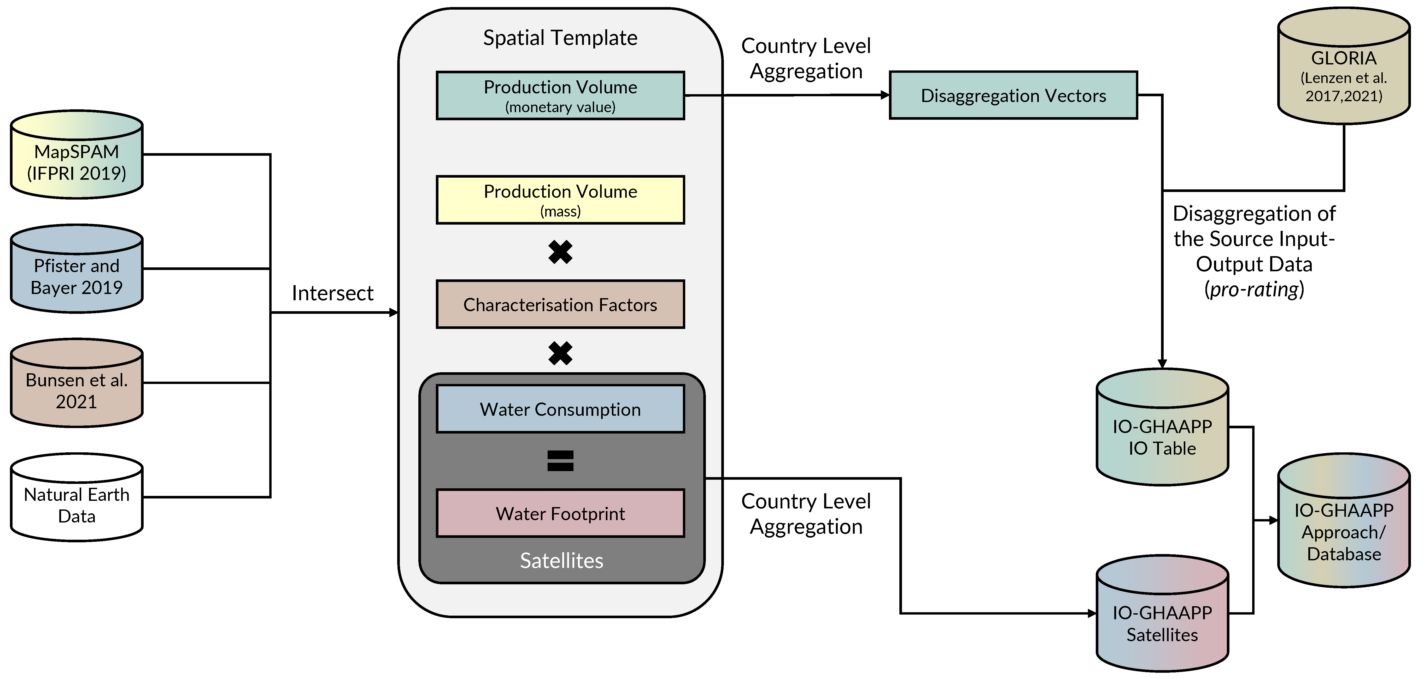
- Integration of the MapSPAM datasets in the GLORIA database: Disaggregating the monetary input–output data from the GLORIA database into the classification of crops of agricultural primary production from the MapSPAM datasets via prorating.
- 2.
- Compilation of water extensions using watershed-level data: Compilation of water extensions for the disaggregated input–output data based on watershed-level data for agricultural primary production, water consumption per agricultural primary production and characterisation factors.
2. Data Sets, Methods and Tools
2.1. Data Sets
2.1.1. Monetary Input–Output Data (GLORIA)
2.1.2. Agricultural Primary Production Produce and Monetary Value (MapSPAM)
2.1.3. Water Consumption of Agricultural Primary Production
2.1.4. Characterisation Factors
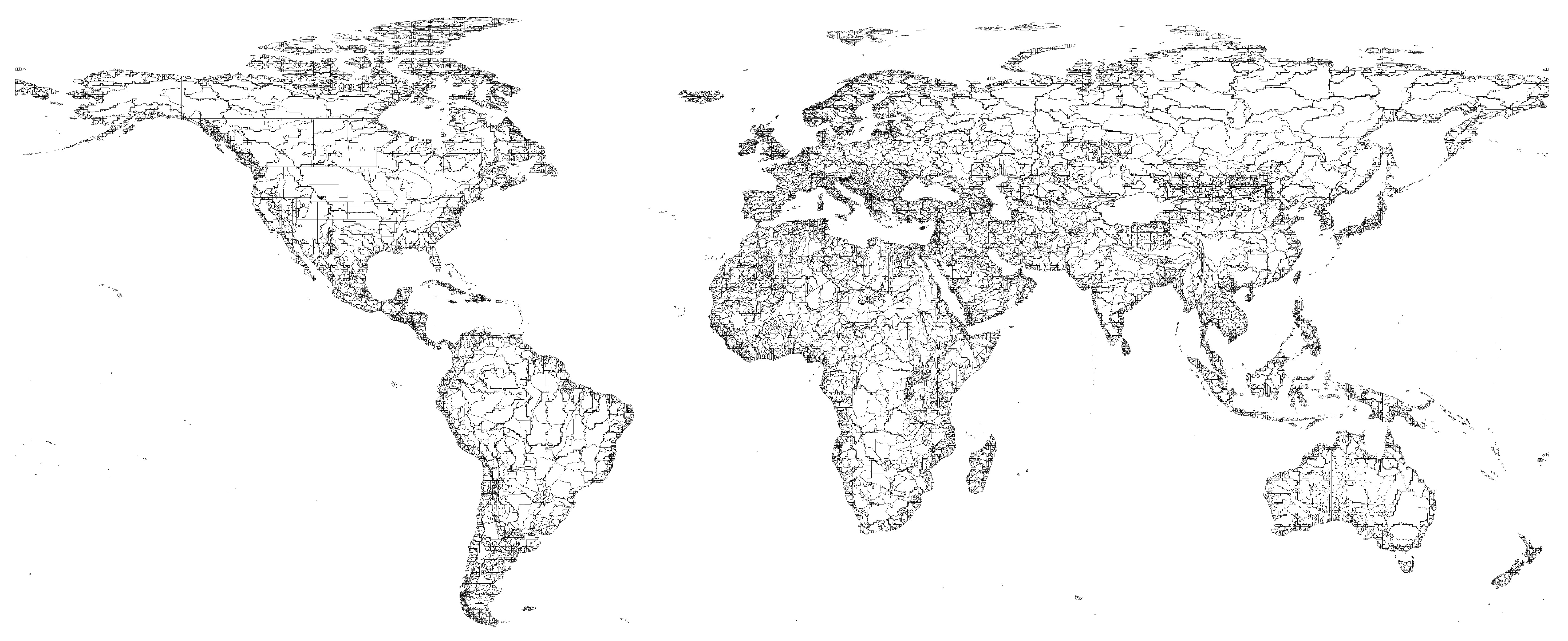
2.1.5. Regional Boundaries
2.2. Data Concordance
2.2.1. Regions
2.2.2. GLORIA Categories, MapSPAM Crops and FAO Crops
2.3. Approaches
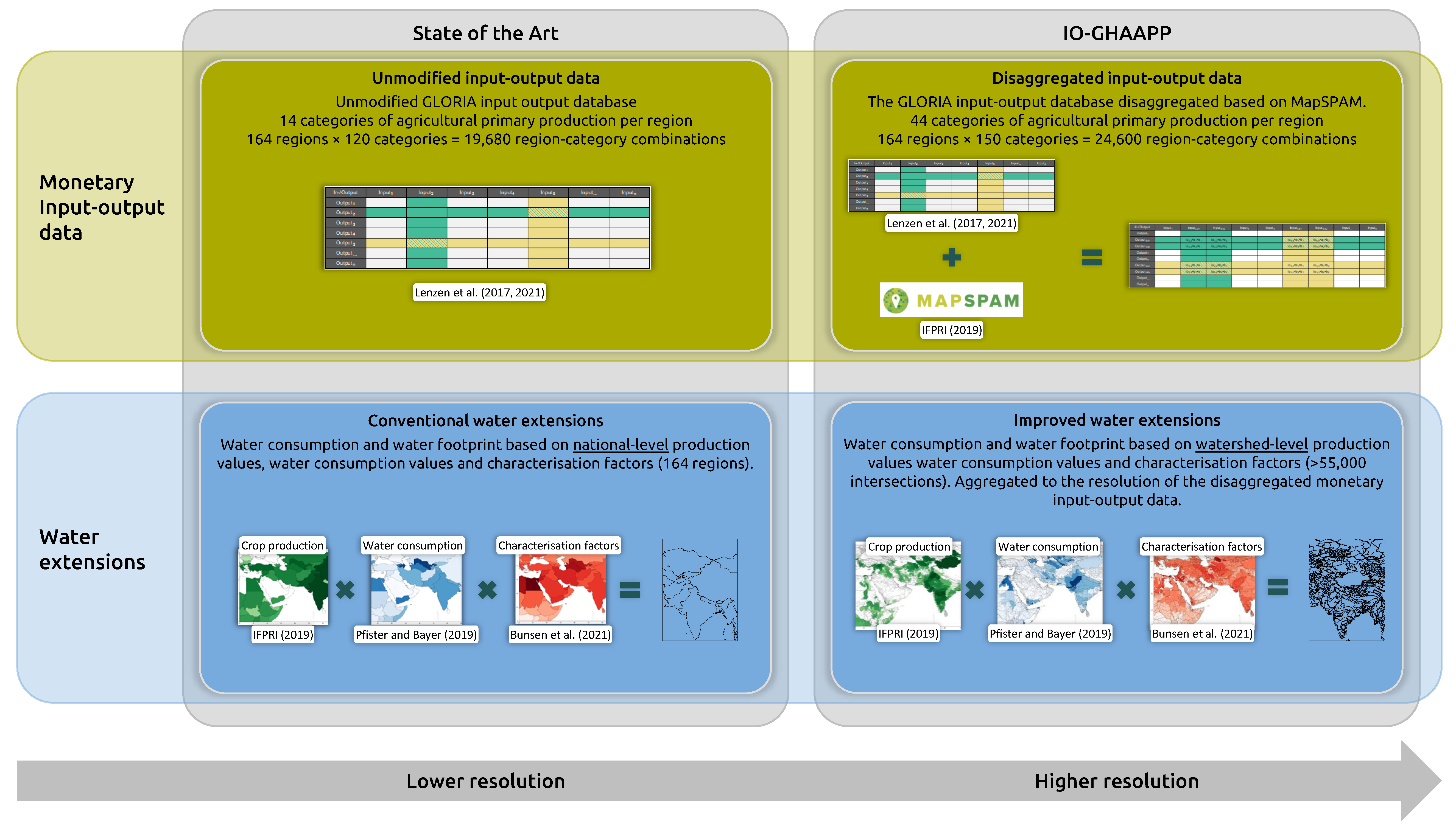
2.3.1. State-of-the-Art Approach
Monetary Input–Output Data
Water Extensions
2.3.2. IO-GHAAPP Approach
Disaggregating the Input–Output Data via Prorating
Extensions (Satellite Accounts)
2.4. Case Study
2.5. Tools
3. Results
3.1. IO-GHAAPP Approach—Transaction Matrix and Final Demand
3.1.1. Disaggregated Monetary Input–Output Data
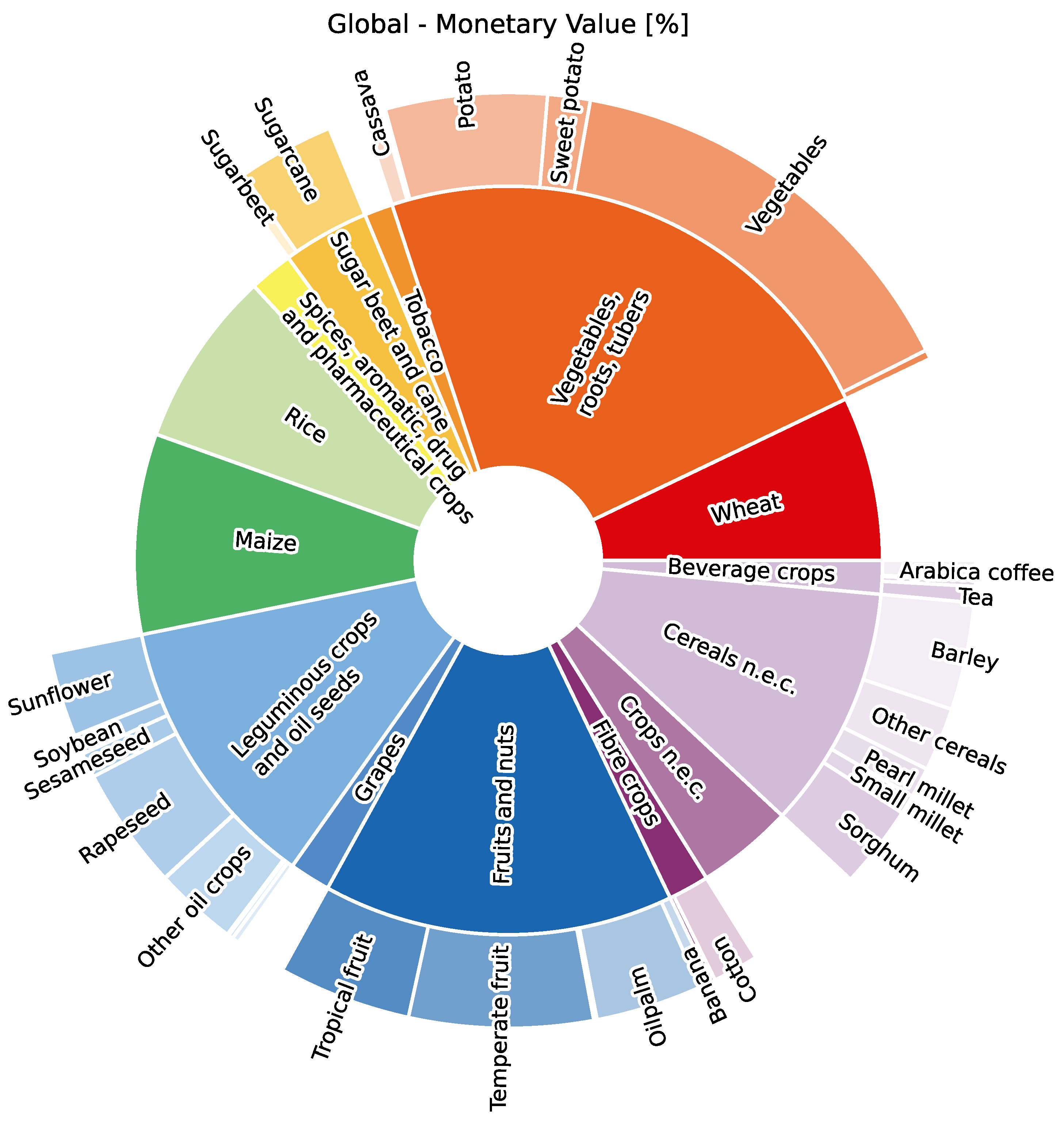
- Growing cereals n.e.c.: Barley (35%), Sorghum (27%), Other cereals (21%), Pearl millet (10%) and Small millet (6%)
- Growing leguminous crops and oil seeds: Rapeseed (35%), Sunflower (24%), Other oil crops (24%), Sunflower (24%), Sesameseed (7%), Soybean (6%) and Coconut (1%)
- Growing vegetables, roots, tubers: Vegetables (64%), Potato (24%), Sweet potato (6%), Cassava (3%), Yams (1%) and Other roots (1%)
- Growing sugar beet and cane: Sugarcane (88%) and Sugarbeet (12%)
- Growing fibre crops: Cotton (90%) and Other fibre crops (10%)
- Growing fruits and nuts: Temperate fruit (42%), Tropical fruit (30%), Oilpalm (24%), Banana (3%) and Plantain (1%)
- Growing beverage crops coffee, tea, etc.: Arabica coffee (44%), Tea (39%), Robusta coffee (14%) and Cocoa (3%)
- United States of America
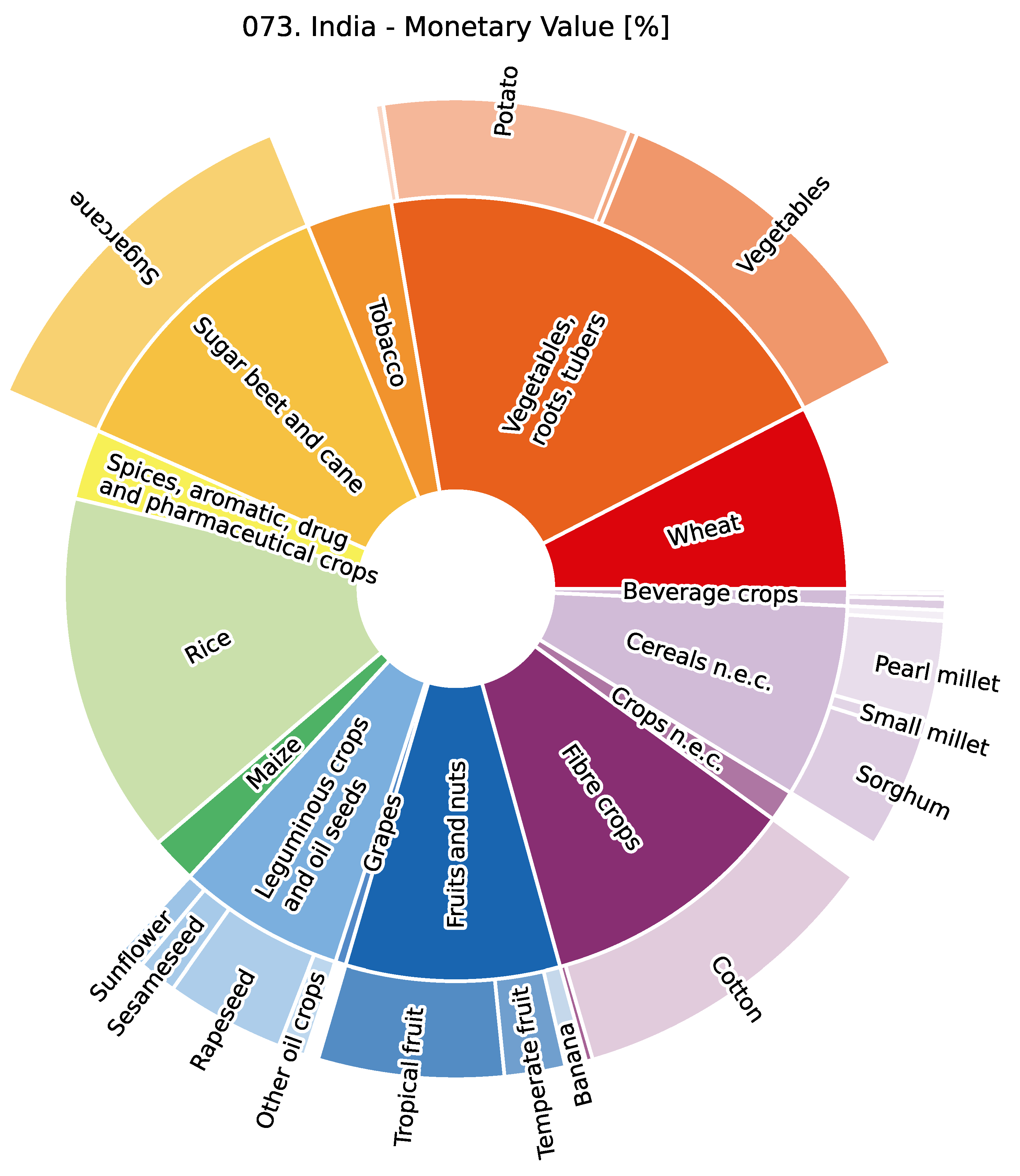
- India
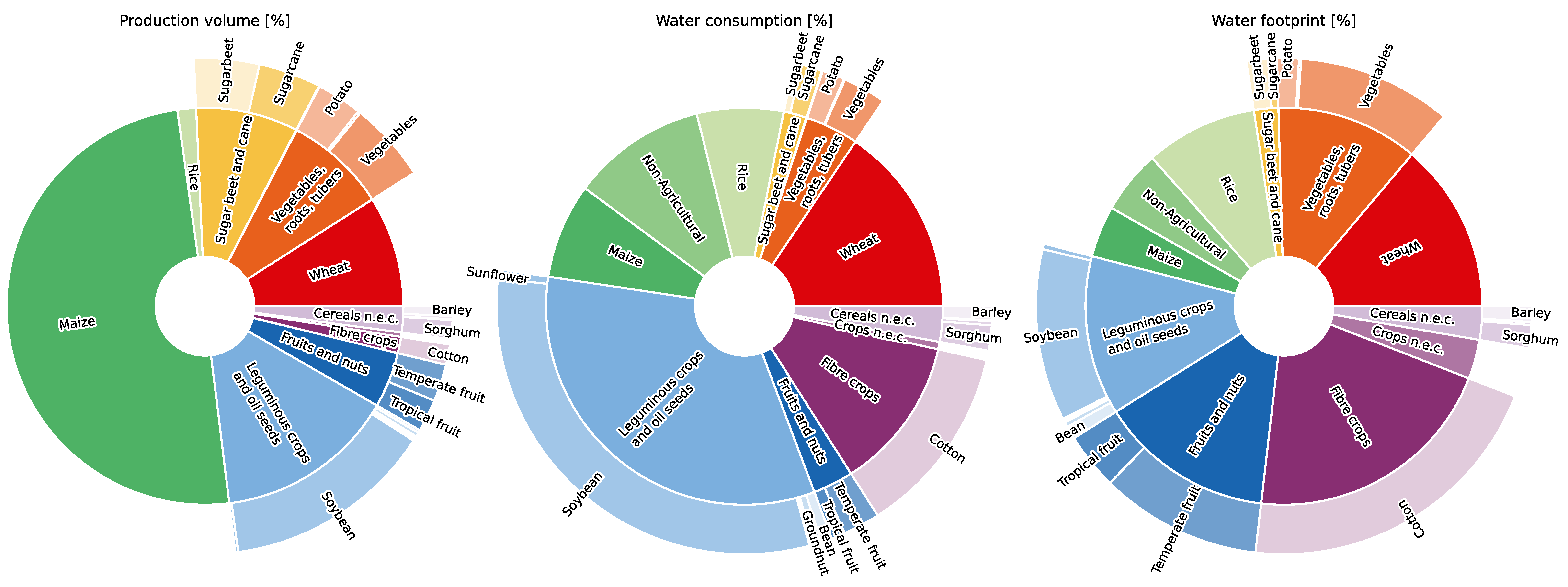
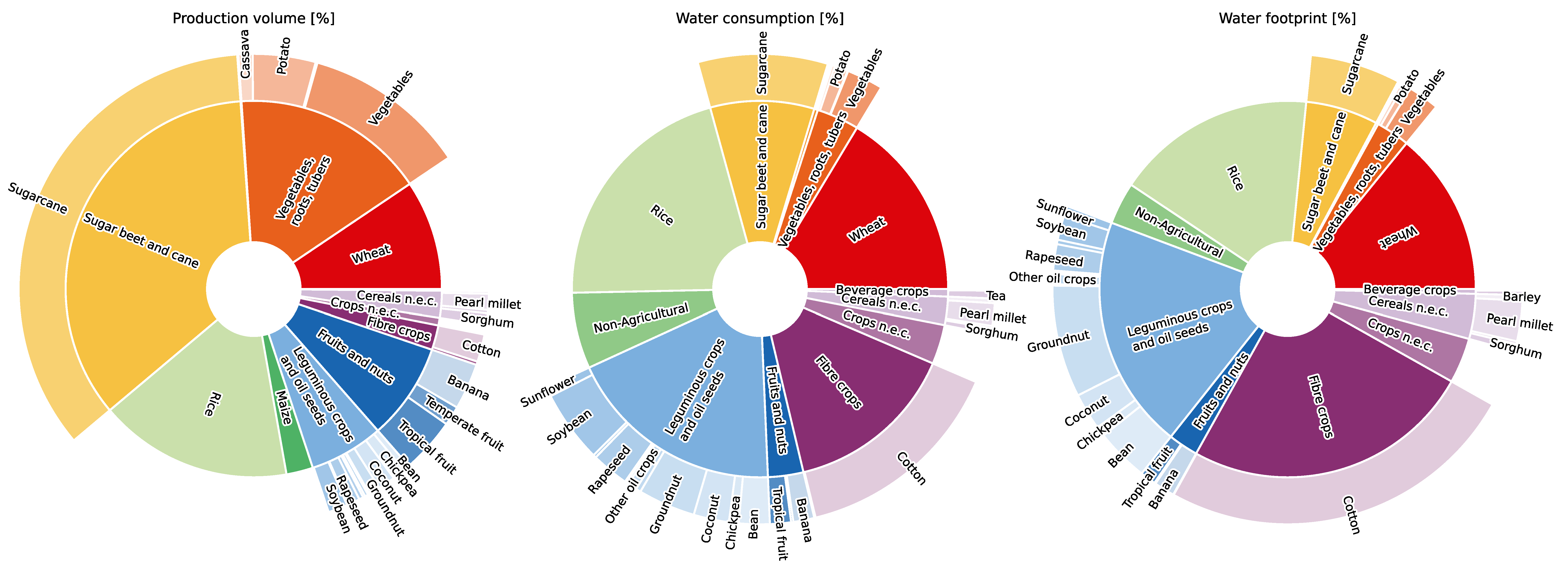
3.2. Extensions (Satellite Accounts)—Production Volume, Water Consumption and Water Footprint
- United States of America
- India
3.3. Water Consumption and Water Footprint—IO-GHAAPP versus State-of-the-Art
- Blue-Water Consumption
- Water Footprint
3.4. IO-GHAAPP Case Study
- Rapeseed
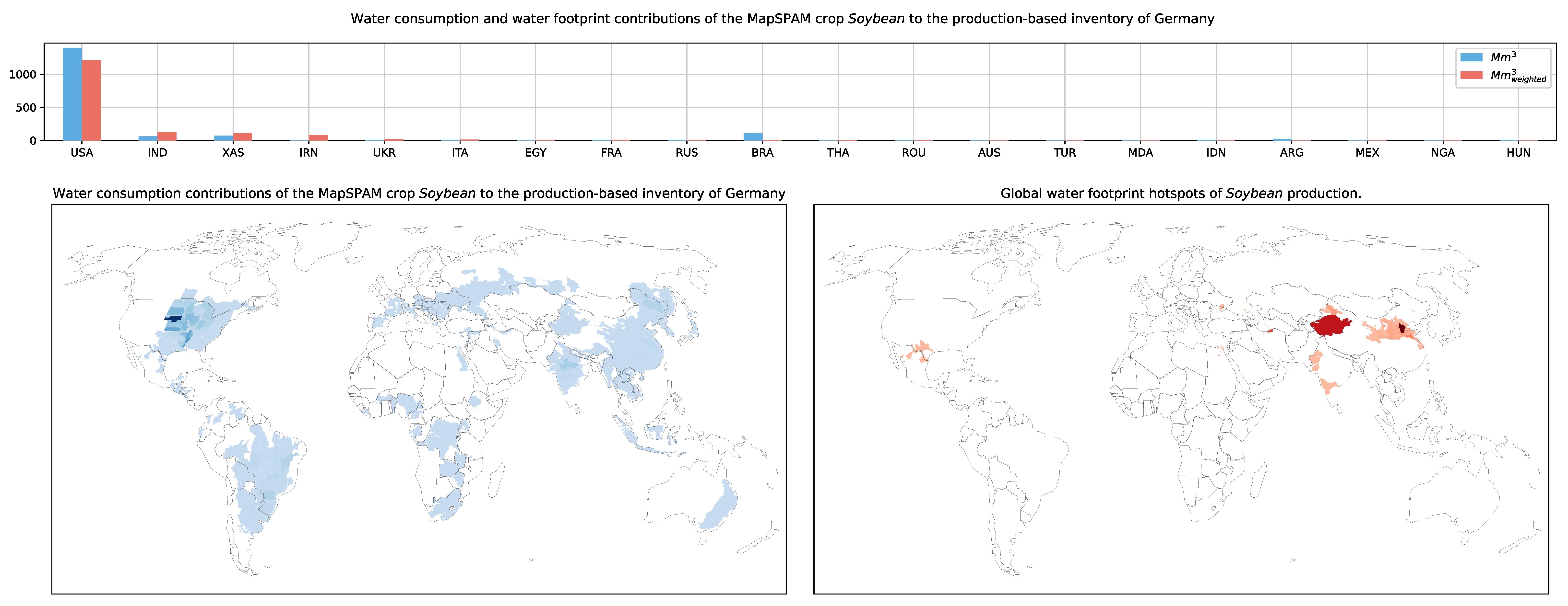
- Soybean
4. Discussion
4.1. Integration of the MapSPAM Model into the GLORIA Database
4.2. IO-GHAAP Approach in Compiling Water Extensions
4.3. Case Study
4.4. Limitations and Suggestions for Future Work
5. Conclusions
Author Contributions
Funding
Data Availability Statement
Acknowledgments
Conflicts of Interest
Abbreviations
| 1MM | One Million |
| CF | Characterisation Factor |
| EE-MRIO | Environmentally Extended Multi-Regional Input–Output (analysis) |
| GLORIA | Global Resource Input Output Assessment (database) |
| IO-GHAAPP | Input–Output Global Hybrid Analysis of Agricultural Primary Production |
| MR-SUT | Multi-Regional Supply-Use Table |
| MapSPAM | Spatial Production Allocation Model |
| USA | United Stated of America |
| USD | United States Dollar |
| WC | Water Consumption (blue-water consumption) |
| WF | Water Footprint |
Appendix A. Supplementary Tables
| MapSPAM Short | MapSPAM Long | FAO Name | FAO Crop Code | Group | Food or Non-Food | GLORIA Category |
|---|---|---|---|---|---|---|
| whea | Wheat | wheat | 15 | cereals | food | 001. Growing wheat |
| maiz | Maize | maize | 56 | cereals | food | 002. Growing maize |
| barl | Barley | barley | 44 | cereals | food | 003. Growing cereals n.e.c |
| pmil | Pearl millet | millet | 79 | cereals | food | 003. Growing cereals n.e.c |
| smil | Small millet | millet | 79 | cereals | food | 003. Growing cereals n.e.c |
| sorg | Sorghum | sorghum | 83 | cereals | food | 003. Growing cereals n.e.c |
| ocer | Other cereals | other cereals ++ | 68, 71, 75, 89, 92, 94, 97, 101, 103, 108 | cereals | food | 003. Growing cereals n.e.c |
| bean | Bean | beans, dry | 176 | pulses | food | 004. Growing leguminous crops and oil seeds |
| chic | Chickpea | chickpea | 191 | pulses | food | 004. Growing leguminous crops and oil seeds |
| cowp | Cowpea | cowpea | 195 | pulses | food | 004. Growing leguminous crops and oil seeds |
| pige | Pigeonpea | pigeon pea | 197 | pulses | food | 004. Growing leguminous crops and oil seeds |
| lent | Lentil | lentils | 201 | pulses | food | 004. Growing leguminous crops and oil seeds |
| opul | Other pulses | broad beans ++ | 181, 187, 203, 205, 210, 211 | pulses | food | 004. Growing leguminous crops and oil seeds |
| soyb | Soybean | soybean | 236 | oilcrops | food | 004. Growing leguminous crops and oil seeds |
| grou | Groundnut | groundnut, with shell | 242 | oilcrops | food | 004. Growing leguminous crops and oil seeds |
| cnut | Coconut | coconut | 249 | oilcrops | food | 004. Growing leguminous crops and oil seeds |
| sunf | Sunflower | sunflower seed | 267 | oilcrops | non-food | 004. Growing leguminous crops and oil seeds |
| rape | Rapeseed | rapeseed | 270, 292 | oilcrops | non-food | 004. Growing leguminous crops and oil seeds |
| sesa | Sesameseed | sesame seed | 289 | oilcrops | non-food | 004. Growing leguminous crops and oil seeds |
| ooil | Other oil crops | olives ++ | 260–339, not 311 and the other oilcrops above | oilcrops | non-food | 004. Growing leguminous crops and oil seeds |
| rice | Rice | rice | 27 | cereals | food | 005. Growing rice |
| pota | Potato | potato | 116 | roots & tubers or starchy roots | food | 006. Growing vegetables, roots, tubers |
| swpo | Sweet potato | sweet potato | 122 | roots & tubers or starchy roots | food | 006. Growing vegetables, roots, tubers |
| yams | Yams | yam | 137 | roots & tubers or starchy roots | food | 006. Growing vegetables, roots, tubers |
| cass | Cassava | cassava | 125 | roots & tubers or starchy roots | food | 006. Growing vegetables, roots, tubers |
| orts | Other roots | yautia ++ | 135, 136, 149 | roots & tubers or starchy roots | food | 006. Growing vegetables, roots, tubers |
| vege | Vegetables | cabbages and other brassicas ++ | 358–463 | vegetables | food | 006. Growing vegetables, roots, tubers |
| sugc | Sugarcane | sugar cane | 156 | sugar crops | non-food | 007. Growing sugar beet and cane |
| sugb | Sugarbeet | sugarbeet | 157 | sugar crops | non-food | 007. Growing sugar beet and cane |
| toba | Tobacco | tobacco leaves | 826 | stimulant | non-food | 008. Growing tobacco |
| cott | Cotton | seed cotton | 328 | fibres | non-food | 009. Growing fibre crops |
| ofib | Other fibre crops | other fibres ++ | 773–821 | fibres | non-food | 009. Growing fibre crops |
| rest | Rest of crops | all individual other crops (eg spices, tree nuts, other sugar crops, mate, rubber) | 161, 216–234, 671,677–839 | non-food | 010. Growing crops n.e.c. | |
| oilp | Oilpalm | palmoil | 254 | oilcrops | non-food | 012. Growing fruits and nuts |
| bana | Banana | banana | 486 | fruits | food | 012. Growing fruits and nuts |
| plnt | Plantain | plantain | 489 | fruits | food | 012. Growing fruits and nuts |
| trof | Tropical fruit | oranges ++ | 490–512, 567–591, 600–603 | fruits | food | 012. Growing fruits and nuts |
| temf | Temperate fruit | apples ++ | 515–560, 592, 619 | fruits | food | 012. Growing fruits and nuts |
| acof | Arabica coffee | coffee | 656 | stimulant | non-food | 013. Growing beverage crops coffee, tea etc |
| rcof | Robusta coffee | coffee | 656 | stimulant | non-food | 013. Growing beverage crops coffee, tea etc |
| coco | Cocoa | cocoa | 661 | stimulant | non-food | 013. Growing beverage crops coffee, tea etc |
| teas | Tea | tea | 667 | stimulant | non-food | 013. Growing beverage crops coffee, tea etc |
| GLORIA Category | MapSPAM Crop | Monetary Value | Production | Water Consumption | Water Footprint | ||||
|---|---|---|---|---|---|---|---|---|---|
| % | % | % | % | ||||||
| Beverage crops | Arabica coffee | 9783 | 44.1 | 4.5 | 26.2 | 5966.7 | 28.0 | 4387.88 | 28.1 |
| Beverage crops | Cocoa | 683 | 3.1 | 4.3 | 25.4 | 4116.9 | 19.0 | 598.09 | 3.8 |
| Beverage crops | Robusta coffee | 3113 | 14.0 | 3.7 | 21.9 | 4025.7 | 19.0 | 1979.05 | 12.7 |
| Beverage crops | Tea | 8603 | 38.8 | 4.5 | 26.5 | 7107.6 | 33.0 | 8640.19 | 55.4 |
| Cereals n.e.c. | Barley | 56,919 | 35.3 | 135.5 | 47.8 | 22,944.4 | 55.0 | 144,091.88 | 59.4 |
| Cereals n.e.c. | Other cereals | 33,913 | 21.0 | 61.3 | 21.6 | 2319.5 | 6.0 | 3825.15 | 1.6 |
| Cereals n.e.c. | Pearl millet | 16,096 | 10.0 | 23.7 | 8.4 | 7514.3 | 18.0 | 61,706.76 | 25.4 |
| Cereals n.e.c. | Small millet | 10,161 | 6.3 | 4.9 | 1.7 | 1216.9 | 3.0 | 6981.98 | 2.9 |
| Cereals n.e.c. | Sorghum | 44,036 | 27.3 | 58.1 | 20.5 | 7568.3 | 18.0 | 25,922.16 | 10.7 |
| Crops n.e.c. | Rest of crops | 64,148 | 100 | 36.0 | 100 | 15,424.0 | 100 | 95,221.0 | 100 |
| Fibre crops | Cotton | 24,417 | 90.4 | 69.6 | 93.5 | 101,380.0 | 100 | 758,967.07 | 99.9 |
| Fibre crops | Other fibre crops | 2586 | 9.6 | 4.8 | 6.5 | 380.3 | 0.0 | 724.12 | 0.1 |
| Fruits and nuts | Banana | 6362 | 2.7 | 105.9 | 10.9 | 12,207.3 | 16.0 | 30,280.37 | 7.9 |
| Fruits and nuts | Oilpalm | 56,292 | 24.2 | 227.3 | 23.3 | 3225.2 | 4.0 | 329.77 | 0.1 |
| Fruits and nuts | Plantain | 1734 | 0.7 | 31.5 | 3.2 | 3642.3 | 5.0 | 1565.37 | 0.4 |
| Fruits and nuts | Temperate fruit | 97,555 | 42.0 | 245.9 | 25.3 | 30,859.2 | 40.0 | 186,631.47 | 48.8 |
| Fruits and nuts | Tropical fruit | 70,514 | 30.3 | 363.3 | 37.3 | 26,740.2 | 35.0 | 163,582.61 | 42.8 |
| Grapes | - | 27,193 | 100 | - | - | - | - | - | - |
| Leguminous crops and oil seeds | Bean | 3749 | 2.0 | 22.8 | 4.2 | 9882.8 | 6.0 | 77,299.94 | 13.1 |
| Leguminous crops and oil seeds | Chickpea | 50 | 0.0 | 11.0 | 2.0 | 4388.7 | 3.0 | 26,916.51 | 4.6 |
| Leguminous crops and oil seeds | Coconut | 2508 | 1.4 | 56.4 | 10.4 | 13,886.1 | 8.0 | 48,371.04 | 8.2 |
| Leguminous crops and oil seeds | Cowpea | 117 | 0.1 | 5.5 | 1.0 | 1127.9 | 1.0 | 1507.94 | 0.3 |
| Leguminous crops and oil seeds | Groundnut | 655 | 0.4 | 40.3 | 7.4 | 24,299.1 | 15.0 | 155,810.46 | 26.5 |
| Leguminous crops and oil seeds | Lentil | 50 | 0.0 | 4.4 | 0.8 | 3724.0 | 2.0 | 18,382.85 | 3.1 |
| Leguminous crops and oil seeds | Other oil crops | 43,821 | 23.7 | 26.6 | 4.9 | 7347.6 | 4.0 | 73,268.37 | 12.4 |
| Leguminous crops and oil seeds | Other pulses | 266 | 0.1 | 20.1 | 3.7 | 2717.8 | 2.0 | 12,026.88 | 2.0 |
| Leguminous crops and oil seeds | Pigeonpea | 8 | 0.0 | 4.0 | 0.7 | 416.3 | 0.0 | 2099.35 | 0.4 |
| Leguminous crops and oil seeds | Rapeseed | 64,894 | 35.1 | 62.3 | 11.5 | 11,821.8 | 7.0 | 37,722.09 | 6.4 |
| Leguminous crops and oil seeds | Sesameseed | 13,146 | 7.1 | 4.4 | 0.8 | 2462.1 | 1.0 | 10,141.57 | 1.7 |
| Leguminous crops and oil seeds | Soybean | 10,379 | 5.6 | 249.9 | 46.0 | 62,695.6 | 38.0 | 77,797.9 | 13.2 |
| Leguminous crops and oil seeds | Sunflower | 44,987 | 24.4 | 35.0 | 6.5 | 19,878.6 | 12.0 | 47,376.41 | 8.0 |
| Maize | Maize | 132,874 | 100 | 852.1 | 100 | 10,982.0 | 100 | 18,445.79 | 100 |
| Non-Agricultural | - | 60,692,749 | 100 | - | - | 111,212.0 | 100 | 174,638.1 | 100 |
| Rice | Rice | 117,048 | 100 | 698.5 | 100 | 153,178.4 | 100 | 484,967.92 | 100 |
| Spices, aromatic, drug and pharmaceutical crops | - | 29,016 | 100 | - | - | - | - | - | - |
| Sugar beet and cane | Sugarbeet | 6729 | 11.7 | 245.0 | 12.5 | 3228.4 | 5.0 | 14,031.3 | 6.8 |
| Sugar beet and cane | Sugarcane | 50,872 | 88.3 | 1715.2 | 87.5 | 63,196.0 | 95.0 | 193,097.69 | 93.2 |
| Tobacco | Tobacco | 18,823 | 100 | 7.2 | 100 | 2731.0 | 100 | 6049.58 | 100 |
| Vegetables, roots, tubers | Cassava | 10,305 | 2.9 | 241.9 | 14.4 | 3294.4 | 5.0 | 5406.39 | 1.9 |
| Vegetables, roots, tubers | Other roots | 1834 | 0.5 | 18.8 | 1.1 | 135.0 | 0.0 | 112.09 | 0.0 |
| Vegetables, roots, tubers | Potato | 85,663 | 24.3 | 345.5 | 20.6 | 18,122.2 | 26.0 | 64,137.88 | 22.2 |
| Vegetables, roots, tubers | Sweet potato | 22,577 | 6.4 | 103.8 | 6.2 | 3640.6 | 5.0 | 4436.04 | 1.5 |
| Vegetables, roots, tubers | Vegetables | 226,724 | 64.4 | 915.2 | 54.6 | 43,792.3 | 63.0 | 214,643.91 | 74.3 |
| Vegetables, roots, tubers | Yams | 4898 | 1.4 | 52.4 | 3.1 | 399.9 | 1.0 | 93.35 | 0.0 |
| Wheat | Wheat | 109,019 | 100 | 673.9 | 100 | 215,350.8 | 100 | 1,107,976.83 | 100 |
| Total | 62,227,870 | 7797 | 1,050,550 | 4,372,193 | |||||
Appendix B. Supplementary Figures

References
- Steffen, W.; Sanderson, R.A.; Tyson, P.D.; Jäger, J.; Matson, P.A., III; Oldfield, F.; Richardson, K.; Schellnhuber, H.J.; Turner, B.L.; Wasson, R.J. Global Change and the Earth System: A Planet Under Pressure; Global Change—The IGBP Series; Springer: Berlin/Heidelberg, Germany, 2004. [CrossRef]
- Steffen, W.; Richardson, K.; Rockstrom, J.; Cornell, S.E.; Fetzer, I.; Bennett, E.M.; Biggs, R.; Carpenter, S.R.; de Vries, W.; de Wit, C.A.; et al. Planetary boundaries: Guiding human development on a changing planet. Science 2015, 347, 1259855. [Google Scholar] [CrossRef] [Green Version]
- Crutzen, P.J. Geology of mankind. Nature 2002, 415, 23. [Google Scholar] [CrossRef]
- Meadows, D.H.; Meadows, D.L.; Randers, J.; Behrens, W.W. The Limits to Growth: A Report for the Club of Rome’s Project on the Predicament of Mankind, 2nd ed.; Universe Books: New York, NY, USA, 1972. [Google Scholar]
- Meadows, D.H.; Randers, J.; Meadows, D.L. The Limits to Growth: The 30-Year Update; Earthscan: London, UK, 2004. [Google Scholar]
- Rockström, J.; Steffen, W.; Noone, K.; Persson, R.; Chapin, F.S.I.; Lambin, E.; Lenton, T.M.; Scheffer, M.; Folke, C.; Schellnhuber, H.J.; et al. Planetary Boundaries: Exploring the Safe Operating Space for Humanity. Ecol. Soc. 2009, 14, 32. [Google Scholar] [CrossRef]
- Steffen, W.; Rockström, J.; Richardson, K.; Lenton, T.M.; Folke, C.; Liverman, D.; Summerhayes, C.P.; Barnosky, A.D.; Cornell, S.E.; Crucifix, M.; et al. Trajectories of the Earth System in the Anthropocene. Proc. Natl. Acad. Sci. USA 2018, 115, 8252–8259. [Google Scholar] [CrossRef] [Green Version]
- Rockström, J.; Karlberg, L. The Quadruple Squeeze: Defining the safe operating space for freshwater use to achieve a triply green revolution in the Anthropocene. Ambio 2010, 39, 257–265. [Google Scholar] [CrossRef] [Green Version]
- Rockström, J.; Falkenmark, M.; Allan, T.; Folke, C.; Gordon, L.; Jägerskog, A.; Kummu, M.; Lannerstad, M.; Meybeck, M.; Molden, D.; et al. The unfolding water drama in the Anthropocene: Towards a resilience based perspective on water for global sustainability. Ecohydrology 2014, 7, 1249–1261. [Google Scholar] [CrossRef]
- Falkenmark, M.; Wang-Erlandsson, L.; Rockström, J. Understanding of water resilience in the Anthropocene. J. Hydrol. X 2019, 2, 100009. [Google Scholar] [CrossRef]
- Bunsen, J.; Berger, M.; Finkbeiner, M. Planetary boundaries for water—A review. Ecol. Indic. 2021, 121, 107022. [Google Scholar] [CrossRef]
- Bunsen, J.; Berger, M.; Ward, H.; Finkbeiner, M. Germany’s global water consumption under consideration of the local safe operating spaces of watersheds worldwide. Clean. Responsible Consum. 2021, 3, 100034. [Google Scholar] [CrossRef]
- Döll, P.; Siebert, S. Global modeling of irrigation water requirements. Water Resour. Res. 2002, 38, 8-1-8-10. [Google Scholar] [CrossRef]
- United Nations. E/CN.17/1997/9 Comprehensive assessment of the freshwater resources of the world—Report of the Secretary-General. In Proceedings of the Commission on Sustainable Development. In Proceedings of the Commission on Sustainable Development, Rio de Janeiro, Brazil, 7–25 April 1997. [Google Scholar]
- UN Water. Sustainable Development Goal 6: Synthesis Report 2018 on Water and Sanitation; United Nations Publications, United Nations: New York, NY, USA, 2018. [Google Scholar]
- United Nations. The United Nations World Water Development Report 2022: Groundwater: Making the Invisible Visible; Technical Report; UNESCO World Water Assessment Programme: Paris, France, 2022. [Google Scholar]
- United Nations. Summary Progress Update 2021—DG 6—Water and Sanitation for All. Version: July 2021. UN-Water 2021. Available online: https://www.unwater.org/publications/summary-progress-update-2021-sdg-6-water-and-sanitation-all (accessed on 4 May 2023).
- United Nations. The United Nations World Water Development Report 2018. 2018. Available online: https://www.unwater.org/publications/world-water-development-report-2018 (accessed on 4 May 2023).
- United Nations. Resolution adopted by the General Assembly on 28 July 2010: 64/292. The Human Right to Water and Sanitation. 2010. Available online: https://documents-dds-ny.un.org/doc/UNDOC/GEN/N09/479/35/PDF/N0947935.pdf?OpenElement (accessed on 4 May 2023).
- WEF. The Global Risks Report 2020. World Economic Forum (WEF) 2020. Available online: https://www.weforum.org/reports/the-global-risks-report-2020/?DAG=3&gclid=EAIaIQobChMIq-iC5_60_wIV31UPAh0i6wSJEAAYAiAAEgJkiPD_BwE (accessed on 4 May 2023).
- WEF. The Global Risks Report 2021. World Economic Forum (WEF) 2021. Available online: https://www.weforum.org/reports/the-global-risks-report-2021/ (accessed on 4 May 2023).
- United Nations. Transforming Our World: The 2030 Agenda for Sustainable Development. Resolution Adopted by the General Assembly 2015. Available online: https://sdgs.un.org/publications/transforming-our-world-2030-agenda-sustainable-development-17981 (accessed on 4 May 2023).
- Ono, Y.; Motoshita, M.; Itsubo, N. Development of water footprint inventory database on Japanese goods and services distinguishing the types of water resources and the forms of water uses based on input-output analysis. Int. J. Life Cycle Assess. 2015, 20, 1456–1467. [Google Scholar] [CrossRef]
- Lutter, S.; Pfister, S.; Giljum, S.; Wieland, H.; Mutel, C. Spatially explicit assessment of water embodied in European trade: A product-level multi-regional input-output analysis. Glob. Environ. Change 2016, 38, 171–182. [Google Scholar] [CrossRef] [Green Version]
- Ridoutt, B.G.; Hadjikakou, M.; Nolan, M.; Bryan, B.A. From Water-Use to Water-Scarcity Footprinting in Environmentally Extended Input–Output Analysis. Environ. Sci. Technol. 2018, 52, 6761–6770. [Google Scholar] [CrossRef]
- Lenzen, M.; Moran, D.; Bhaduri, A.; Kanemoto, K.; Bekchanov, M.; Geschke, A.; Foran, B. International trade of scarce water. Ecol. Econ. 2013, 94, 78–85. [Google Scholar] [CrossRef]
- Lenzen, M. An input–output analysis of Australian water usage. Water Policy 2001, 3, 321–340. [Google Scholar] [CrossRef]
- Leontief, W. Quantitative input and output relations in the economic systems of the United States. Rev. Econ. Stat. 1936, 18, 105–125. [Google Scholar] [CrossRef] [Green Version]
- Leontief, W. Environmental Repercussions and the Economic Structure: An Input-Output Approach. Rev. Econ. Stat. 1970, 52, 262–271. [Google Scholar] [CrossRef]
- Miller, R.E.; Blair, P.D. Input–Output Analysis: Foundations and Extensions, 2nd ed.; Cambridge University Press: Cambridge, UK, 2009; p. 784. [Google Scholar]
- Bunsen, J.; Finkbeiner, M. An Introductory Review of Input-Output Analysis in Sustainability Sciences Including Potential Implications of Aggregation. Sustainability 2023, 15, 46. [Google Scholar] [CrossRef]
- Oosterhaven, J. A family of square and rectangular interregional input-output tables and models. Reg. Sci. Urban Econ. 1984, 14, 565–582. [Google Scholar] [CrossRef]
- Lenzen, M. Aggregation Versus Disaggregation in Input–Output Analysis of the Environment. Econ. Syst. Res. 2011, 23, 73–89. [Google Scholar] [CrossRef]
- Peters, G.P.; Andrew, R.; Lennox, J. Constructing an Environmentally-Extended Multi-Regional Input–Output Table Using the Gtap Database. Econ. Syst. Res. 2011, 23, 131–152. [Google Scholar] [CrossRef]
- De Koning, A.; Bruckner, M.; Lutter, S.; Wood, R.; Stadler, K.; Tukker, A. Effect of aggregation and disaggregation on embodied material use of products in input–output analysis. Ecol. Econ. 2015, 116, 289–299. [Google Scholar] [CrossRef]
- Schoer, K.; Dittrich, M.; Limberger, S.; Ewers, B.; Kovanda, J.; Weinzettel, J. Disaggregating Input-Output Tables for the Calculation of Raw Material Footprints: Minimum Requirements, Possible Methods, Data Sources and a Proposed Method for Eurostat: 2021 Edition; Eurostat (European Commission) Publication Office of the European Union: Luxembourg, 2021. [Google Scholar]
- Boulay, A.M.; Bare, J.; Benini, L.; Berger, M.; Lathuillière, M.J.; Manzardo, A.; Margni, M.; Motoshita, M.; Núñez, M.; Pastor, A.V.; et al. The WULCA consensus characterization model for water scarcity footprints: Assessing impacts of water consumption based on available water remaining (AWARE). Int. J. Life Cycle Assess. 2018, 23, 368–378. [Google Scholar] [CrossRef] [Green Version]
- Berger, M.; Eisner, S.; van der Ent, R.; Flörke, M.; Link, A.; Poligkeit, J.; Bach, V.; Finkbeiner, M. Enhancing the Water Accounting and Vulnerability Evaluation Model: WAVE+. Environ. Sci. Technol. 2015, 52, 10757–10766. [Google Scholar] [CrossRef] [Green Version]
- Tukker, A.; Dietzenbacher, E. Global Multiregional Input-Output Frameworks: An Introduction and Outlook. Econ. Syst. Res. 2013, 25, 1–19. [Google Scholar] [CrossRef] [Green Version]
- Lenzen, M.; Moran, D.; Kanemoto, K.; Geschke, A. Building Eora: A global multi-region input-output database at high country and sector resolution. Econ. Syst. Res. 2013, 25, 20–49. [Google Scholar] [CrossRef]
- Lenzen, M.; Kanemoto, K.; Moran, D.; Geschke, A. Mapping the Structure of the World Economy. Environ. Sci. Technol. 2012, 46, 8374–8381. [Google Scholar] [CrossRef]
- Stadler, K.; Wood, R.; Bulavskaya, T.; Södersten, C.J.; Simas, M.; Schmidt, S.; Usubiaga, A.; Acosta-Fernández, J.; Kuenen, J.; Bruckner, M.; et al. EXIOBASE 3: Developing a Time Series of Detailed Environmentally Extended Multi-Regional Input-Output Tables: EXIOBASE 3. J. Ind. Ecol. 2018, 22, 502–515. [Google Scholar] [CrossRef] [Green Version]
- Bruckner, M.; Wood, R.; Moran, D.; Kuschnig, N.; Wieland, H.; Maus, V.; Börner, J. FABIO—The Construction of the Food and Agriculture Biomass Input–Output Model. Environ. Sci. Technol. 2019, 53, 11302–11312. [Google Scholar] [CrossRef] [Green Version]
- Lenzen, M.; Geschke, A.; Abd Rahman, M.D.; Xiao, Y.; Fry, J.; Reyes, R.; Dietzenbacher, E.; Inomata, S.; Kanemoto, K.; Los, B.; et al. The Global MRIO Lab—Charting the world economy. Econ. Syst. Res. 2017, 29, 158–186. [Google Scholar] [CrossRef]
- Lenzen, M.; Geschke, A.; West, J.; Fry, J.; Malik, A.; Giljum, S.; Milà i Canals, L.; Piñero, P.; Lutter, S.; Wiedmann, T.; et al. Implementing the material footprint to measure progress towards Sustainable Development Goals 8 and 12. Nat. Sustain. 2021, 5, 157–166. [Google Scholar] [CrossRef]
- Lewandowski, I.; Lippe, M.; Montoya, J.C.; Dickhöfer, U.; Langenberger, G.; Pucher, J.; Schließmann, U.; Schmid-Staiger, U.; Derwenskus, F.; Lippert, C. Primary Production. In Bioeconomy: Shaping the Transition to a Sustainable, Biobased Economy; Lewandowski, I., Ed.; Springer International Publishing: Cham, Switzerland, 2018; pp. 97–178. [Google Scholar] [CrossRef] [Green Version]
- Hoekstra, A.; Chapagain, A.; Aldaya, M.; Mekonnen, M. The Water Footprint Assessment Manual: Setting the Global Standard, 1st ed.; Routledge: Oxfordshire, UK, 2011. [Google Scholar] [CrossRef]
- International Food Policy Research Institute. Global Spatially-Disaggregated Crop Production Statistics Data for 2010 Versio 2.0; International Food Policy Research Institute: Washington, DC, USA, 2019. [Google Scholar] [CrossRef]
- Pfister, S.; Bayer, P. Water consumption of crop on watershed level (blue and green water, uncertainty, incl. shapefile) and monthly irrigation water consumption. Mendeley Data 2019, 3. [Google Scholar] [CrossRef]
- Natural Earth—Free Vector and Raster Map Data at 1:10m, 1:50m, and 1:110m Scales. Available online: https://www.naturalearthdata.com/ (accessed on 4 May 2023).
- Perry, M. Rasterstats. 2023. Available online: https://github.com/perrygeo/python-rasterstats (accessed on 4 May 2023).
- UN Statistics Division. Handbook of Input-Output Table Compilation and Analysis; UN Statistics Division: Paris, France, 1999. [Google Scholar]
- Harris, C.R.; Millman, K.J.; van der Walt, S.J.; Gommers, R.; Virtanen, P.; Cournapeau, D.; Wieser, E.; Taylor, J.; Berg, S.; Smith, N.J.; et al. Array programming with NumPy. Nature 2020, 585, 357–362. [Google Scholar] [CrossRef]
- Reback, J.; Jbrockmendel; McKinney, W.; Van Den Bossche, J.; Augspurger, T.; Cloud, P.; Hawkins, S.; Gfyoung; Roeschke, M.; Sinhrks; et al. pandas-dev/pandas: Pandas 1.3.4. Zenodo 2021. [Google Scholar] [CrossRef]
- Jordahl, K.; Van den Bossche, J.; Wasserman, J.; McBride, J.; Gerard, J.; Tratner, J.; Perry, M.; Farmer, C.; Cochran, M.; Gillies, S.; et al. geopandas/geopandas: V0.4.1. Zenodo 2019. [Google Scholar] [CrossRef]
- Hunter, J.D. Matplotlib: A 2D graphics environment. Comput. Sci. Eng. 2007, 9, 90–95. [Google Scholar] [CrossRef]
- Pfister, S.; Koehler, A.; Hellweg, S. Assessing the Environmental Impacts of Freshwater Consumption in LCA. Environ. Sci. Technol. 2009, 43, 4098–4104. [Google Scholar] [CrossRef] [Green Version]


Disclaimer/Publisher’s Note: The statements, opinions and data contained in all publications are solely those of the individual author(s) and contributor(s) and not of MDPI and/or the editor(s). MDPI and/or the editor(s) disclaim responsibility for any injury to people or property resulting from any ideas, methods, instructions or products referred to in the content. |
© 2023 by the authors. Licensee MDPI, Basel, Switzerland. This article is an open access article distributed under the terms and conditions of the Creative Commons Attribution (CC BY) license (https://creativecommons.org/licenses/by/4.0/).
Share and Cite
Bunsen, J.; Coroamă, V.; Finkbeiner, M. Input–Output Global Hybrid Analysis of Agricultural Primary Production (IO-GHAAPP) Database. Sustainability 2023, 15, 9351. https://doi.org/10.3390/su15129351
Bunsen J, Coroamă V, Finkbeiner M. Input–Output Global Hybrid Analysis of Agricultural Primary Production (IO-GHAAPP) Database. Sustainability. 2023; 15(12):9351. https://doi.org/10.3390/su15129351
Chicago/Turabian StyleBunsen, Jonas, Vlad Coroamă, and Matthias Finkbeiner. 2023. "Input–Output Global Hybrid Analysis of Agricultural Primary Production (IO-GHAAPP) Database" Sustainability 15, no. 12: 9351. https://doi.org/10.3390/su15129351