Numerical Analysis of the Effect of Groundwater Seepage on the Active Freezing and Forced Thawing Temperature Fields of a New Tube–Screen Freezing Method

Abstract

To more comprehensively explore the mechanism of the active freezing and thawing process of a new tube–curtain freezing method in construction, the temperature field of the new tube–curtain freezing process is analyzed using finite element software to establish a numerical model. Six paths were set up upstream and downstream of the model and around the top steel tube to analyze the development of frozen soil curtains during active freezing and forced thawing. The results show that, due to the effect of seepage, the cold energy generated by the upstream frozen pipe will be carried to downstream by water, which leads to the asymmetry of the frozen soil curtain. A greater seepage rate leads to a more pronounced the influence on the development of the temperature field. During the process of forced thawing, the first 15 days of the frozen soil curtain heating rate are fastest; thus, it is necessary to monitor the thawing settlement intensively during this period. By comparing different heads of water and different forced thawing temperatures, it was found that a bigger head of water results in a longer thawing time. At a constant head of water, a higher thawing temperature results in a shorter thawing time, with the thawing time at 50 °C being about 0.5 times that at 5 °C. Low-temperature thawing can be chosen to control the cost; however, when the head of water is large, high-temperature thawing can significantly shorten the thawing time. In addition, the new tube–curtain freezing method has little influence on the surrounding environment, along with a short construction period and low construction cost, in accordance with the concept of sustainable development.

1. Introduction

Artificial ground-freezing technology uses artificial refrigeration technology to make the water in the ground freeze, changing the natural rock and soil into natural frozen soil to increase its strength and stability, as well as separate underground water from underground construction. This is a special construction technology used to excavate underground engineering under the protection of a freezing wall, whose essence is the use of artificial refrigeration technology to temporarily change the rock and soil properties to consolidate the stratum [1]. Artificial ground freezing technology is widely used in underground engineering construction because of its small influence on the environment, good waterproofing, and other characteristics [2]. However, when the volume of construction frozen soil is too large, the soil expands excessively when it freezes, and produces settlement displacement when it melts [3,4,5]. To reduce the influence of frost heaving and thawing settlement on construction, scholars combined the tube–curtain method with a freezing method to create the tube–curtain freezing method [6]. This method adopts the characteristics of the freezing method such as good waterproofing and recovery, but also has the high supporting strength of the steel tube, which ensures sufficient supporting force during active freezing and thawing. With the development and utilization of underground space, the application of artificial freezing technology in tunnel construction has become more and more mature [7,8,9]. The Gongbei Tunnel of the Hong Kong–Zhuhai–Macao Bridge used tube–curtain freezing technology for the first time in the world [10,11,12,13]; the process involved jacking the steel tube into the soil to improve the bearing capacity, and then allowing the freezing pipe to cool the soil, which improved the waterproofing and stability after freezing reinforcement, thereby forming the “frozen soil tube–curtain” composite support structure [14,15,16]. In recent years, relevant scholars have carried out in-depth studies and experimental demonstrations related to the construction of the tube–curtain freezing method [17,18,19,20], including control of the tube freezing limit [21,22], steel pipe jacking [23], and temperature monitoring [24]. These findings have played a positive role in promoting the popularization and application of the tube–curtain freezing method. However, the tube–curtain structure studied in this paper was upgraded on the basis of an existing tube–curtain structure; hence, a structure analysis was needed to ensure the accuracy of the experimental results. Existing articles did not analyze and study the thawing temperature field after the construction of the tube–curtain freezing method. For example, the authors of [25] only analyzed the development law of the freezing temperature field, later verifying it using model tests. This paper innovatively adds a temperature field thawing analysis, considering the influence of seepage velocity and thawing temperature on the development of the temperature field; moreover, the time required for complete thawing of the frozen curtain is simulated. The objective of this paper is to provide theoretical and technical guidance for the construction of the Sanya estuary tunnel. The goal is to anticipate the conditions encountered during the construction of the project through numerical simulations in order to propose countermeasures at an earlier stage. It is also hoped to provide technical and theoretical guidance for the construction of a subsea tunnel in a waterfront city. The construction process is shown in Figure 1. The use of the freezing method for underground construction is more environmentally friendly considering characteristics such as no pollution to the surrounding environment, no foreign matter into the soil, and less noise. After the freezing process, the permafrost curtain melts away without affecting the underground structures around the building. In addition, the ends of the construction can be reinforced with nano-silica-doped highly alkaline white cement slurry composites [26] and waterproofed with waste polymer asphalt [27], consistent with the concept of sustainable development.

2. Coupling Theory

In this paper, the temperature field and seepage field were involved in the simulation process; accordingly, we explain the temperature field, seepage field, and their coupling.

2.1. Temperature Field

It is stipulated that the soil is saturated with homogeneous isotropic sand, and the temperature field is influenced by the heat transfer of sand particles and seawater seepage. The volume ratio of seawater and sand particles during sand seepage freezing is $(1-{\mathsf{\theta }}_{\mathrm{S}})/{\mathsf{\theta }}_{\mathrm{S}}$; thus, the differential equation of the temperature field during heat transfer is [28]

$$\begin{array}{c}{C}_{eq}\frac{\alpha T}{\alpha \tau }={\lambda }_{eq}\left(\frac{{\alpha }^{2}T}{\alpha x^2}+\frac{{\alpha }^{2}T}{\alpha y^2}\right)-\left({\rho }_w{C}_w\right)\left(V_x\frac{\alpha T}{\alpha x}+V_y\frac{\alpha T}{\alpha y}\right)\end{array}$$

(1)

where T is the temperature, τ is the time, C_eq is the equivalent volume heat capacity of saturated sand, λ_eq is the equivalent thermal conductivity, ${\rho }_w$ is the density of water, C_w is the specific heat capacity of water, and V_x and V_y are the seepage rate of water.

The porous media heat transfer module in COMSOL Multiphysics 5.4 software was selected for the analysis of heat transfer during sand seepage freezing, which features the following equations [28]:

$$\begin{array}{c}{\left(\rho C_p\right)}_{eff}\frac{\alpha T}{\alpha t}+\rho C_{p}u·\nabla T+\nabla ·q=Q+Q_{vd}\end{array}$$

(2)

$$\begin{array}{c}q=-k_{eff}\nabla T\end{array}$$

(3)

$$\begin{array}{c}{\left(\rho C_p\right)}_{eff}=C_{eq}\end{array}$$

(4)

$$\begin{array}{c}{k}_{eff}={\lambda }_{eq}\end{array}$$

(5)

where ∇ is the Hamiltonian operator, k_eff is the equivalent thermal conductivity, and Q, Q_vd are various source items.

During the process of icing saturated sand, the phase transition of water freezing occurs, and the physical parameters of frosted sand change along with the latent heat of the phase transition. The temperature change during freezing is a transient heat conduction problem. When the soil particle temperature around the porosity of the soil is lower than the liquid temperature within the porosity, according to the knowledge of heat transfer, heat transfer occurs between the fluid and solid due to the temperature difference. The liquid outputs heat to the surrounding solids through heat exchange. The pore water–ice phase transition is formed, thereby completing the freezing process. The thermal equilibrium equation considering the phase transition can, therefore, be established [28]:

$$\begin{array}{c}{C}_{eq}\frac{\alpha T}{\alpha \tau }+{\rho }_{w}L\frac{\alpha {\theta }_W}{\alpha T}+\nabla \left({\rho }_w{C}_{w}uT-{\lambda }_{eq}\nabla T\right)=Q\end{array}$$

(6)

where L is the phase transition latent heat of water icing, θ_w is the amount of water flowing in a unit volume, and Q is the heat source.

2.2. Seepage Field

During the freezing of submarine soil, the seepage of seawater in the sandy soil follows Darcy’s law [28]:

$$\begin{array}{c}Q=K\ast A\ast \frac{\Delta H}{L}\end{array}$$

(7)

where Q is the seepage quantity, A is the cross-sectional area perpendicular to the direction of seepage, H is the head of water, L is the seepage path, and K is the infiltration coefficient.

When analyzing groundwater seepage in COMSOL software, Duthie’s law module was selected, featuring the following partial differential equations [28]:

$$\begin{array}{c}\frac{\partial }{{\partial }_t}\left({ϵ}_p\rho \right)+\nabla ·\left(\rho u\right)=Q_m\end{array}$$

(8)

$$\begin{array}{c}u=-\frac{K}{\eta }\nabla p\end{array}$$

(9)

where p is the pore water pressure in Pa, Q_m denotes the various source terms in W/m³, K is the permeability coefficient of the soil in m/s, and η is the viscosity of water in kg/(m∙s).

In the formula, the sand layer permeability coefficient K changes with temperature during freezing, which means that the permeability coefficient can be expressed as a function of temperature change; therefore, the coupling of the temperature field and seepage field can be represented by this functional relation. When the water–ice phase transition occurs during soil freezing, the coupling relationship between the permeation field and the temperature field is described by the Heaviside step function [28]:

$$\begin{array}{c}K\left(T\right)=K_{U}H\left(T\right)+K_f\left(1-H\left(T\right)\right)\end{array}$$

(10)

where K and k are the permeability coefficients of sand and frozen sand, respectively, in units of $\mathrm{m}/\mathrm{s}$. Accordingly, $H\left(T\right)=flc2hs(T-T_d,\delta T)$, where T is the temperature of the sand, T is the temperature of the transformation point, and ΔT is the radius of the transformation zone.

2.3. Coupling of Temperature and Percolation Fields

The interaction between the two fields in the coupling process is constrained by two main aspects. On the one hand, the change in seepage field in the soil system will make the seepage water flow participate in the heat transfer and exchange in the soil system, thus affecting the distribution of the temperature field. On the other hand, the temperature field changes in the soil system and the temperature gradient cause the movement of water to change the osmotic coefficient of the soil system. The modulus of elasticity and strength of the soil are functions of temperature; hence, the temperature change will also lead to a change in the seepage field of the soil system.

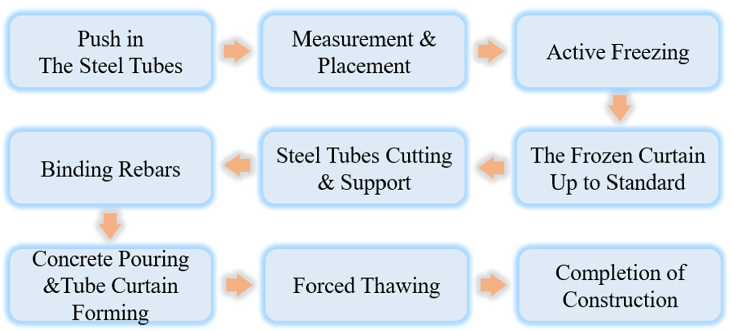
3. Project Overview and Numerical Modeling

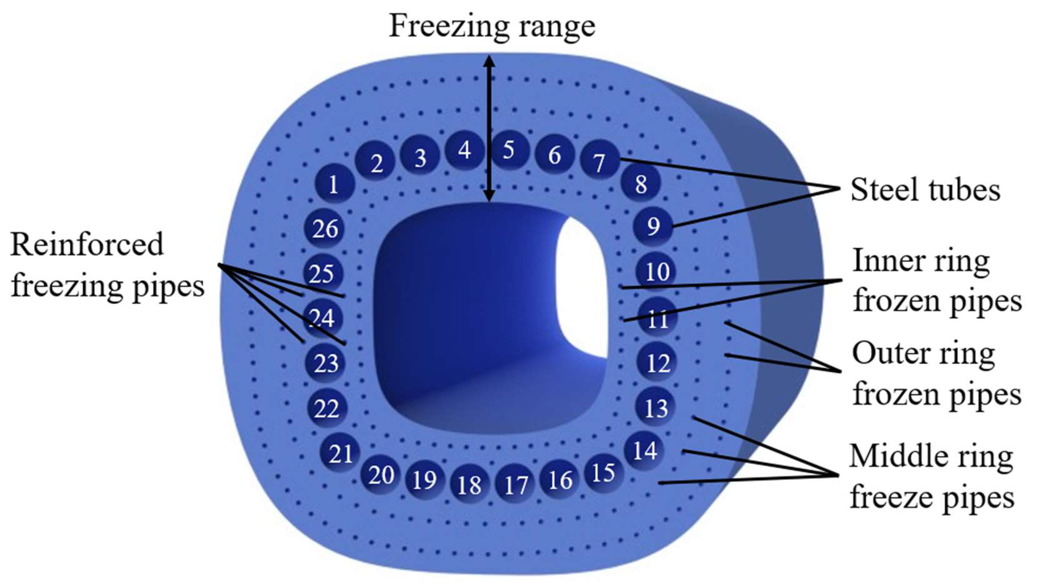
3.1. Project Overview

The Sanya estuary passage project is located in Tianya District, Sanya City, across the mouth of the Sanya River, connecting the western part of the river with Luhuitou Peninsula. The total length of the tunnel is 3180 m (including ramps and pedestrian passage), the road grade for the city is trunk road, the design speed is 40 km/h, with four lanes in both directions, the minimum flat curve radius is 70 m, and the maximum longitudinal slope is 6%. According to the wiring conditions on both sides of the Sanya estuary tunnel, the preliminary design of the estuary section of the tunnel was a single-cavern double tunnel with upper and lower stacked layers, using the pipe curtain structure method of construction. The main design parameters of the tube–curtain structure were as follows: the external dimension of the structure was 17.3 × 17.3 m, the circumferential arrangement of 26 steel tubes was 2.0 m in outer diameter and 20 mm in wall thickness, the secondary lining was made of C50 concrete, the wall thickness was 1.0 m, and the plate thickness was 0.7 m; the preliminary design of the tube–curtain structure is shown in Figure 2. The freezing construction was carried out before cutting the steel tube. The freezing pipe was arranged in three layers; 96 φ127 freezing pipes were uniformly arranged on the outer ring, 76 φ127 freezing pipes were uniformly arranged on the middle ring, and 58 φ127 freezing pipes were uniformly arranged on the inner ring. In addition, 58 inter-tubular strengthening freezing tubes were arranged both inside and outside of the steel pipe. The effective thickness of the freezing curtain was 4.5 m, and the average temperature of the freezing curtain was less than −13 °C. The frozen soil needed to have good uniformity, self-independence, and the necessary strength. When the freezing curtain meets the design requirements, the maintenance freezing stage begins, steel pipes are cut, support is completed, and steel tubes are filled with concrete. Freezing cannot be stopped during this period, until the inner lining of the tube–curtain section is completed and achieves the design strength. The groundwater of this construction site is closely connected with river and seawater hydraulically. The groundwater level changes significantly with the seasonal climate and the dynamic changes in river water level. According to the regional hydrogeological data, the annual variation of groundwater level in this area is about 1–3 m. At the beginning of the investigation, the water level was 1.30–8.00 m (average 3.16 m), the elevation ranged from −0.67 to 1.60 (average 0.48 m), the depth of the stable water level was 1.30–8.20 m (average 3.36 m), and the elevation ranged from −0.77 to 1.50 m (average 0.29 m). Heads of water of 1 m, 2 m, and 3 m were selected for numerical analysis.

3.2. Construction of the Numerical Model

COMSOL Multiphysics was used to establish a transient 3D thermal conductivity model, with the phase transition, geometric model size, and freezing pipe arrangement determined according to the engineering profile. To simplify the calculation, the geometry w chosen as the length in the X-axis direction × width in the Y-axis direction × depth in the Z-axis direction = 30 × 30 × 10 m. The freezing tube was set to a radius of 0.05 m and a length of 10 m, with a total of 230 tubes. The numerical model is shown in Figure 3. According to the hydrothermal coupled freezing model study by Pimentel [29], it is known that the numerical simulation of the development of the temperature field under seepage conditions by hydrothermal coupling is feasible. Similar studies such as [30,31,32,33,34] applied active freezing and forced thawing in underground engineering construction and compared the measured data of temperature field development with the simulated data through model tests, and the comparison results matched reasonably well; therefore, the numerical simulation can realistically reflect the actual engineering profile.

3.3. Basic Assumptions for Numerical Calculation

Freezing under seepage conditions is a complex and intertwined process with various factors. Therefore, to investigate the effect of groundwater seepage rate on the freezing temperature field and thawing and to simplify the calculation, certain assumptions are made on the numerical simulation process:

• The most unfavorable soil parameters are selected for simulation, assuming that the area of freezing is saturated soil, and the soil is continuous, uniform, and isotropic;
• The brine temperature is always considered to be the temperature of the outer wall of the frozen pipe, ignoring the heat loss caused by convective heat transfer of brine;
• The seepage field within the frozen area conforms to Darcy’s law, and the seepage velocity approaches zero after the soil freezes;
• The effect of the stress field on the temperature field is neglected, considering only the coupling effect of the temperature field and seepage field;
• According to the project profile, it is assumed that the formation of permafrost curtain starts at −1 °C, and that the formation of permafrost curtain in the area within the −13 °C isotherm meets the excavation conditions;
• There is no freezing deflection of the frozen pipe during the freezing process of the model, along with uniform unidirectional seepage of water flow, and no heat loss during the freezing process.

3.4. Parameter Selection

The physical parameters of the soil were obtained from the permafrost test, and it was found that the thermal conductivity of fine sand and gravel sand ranged from 2.259 to 4.653 W/(m·K), corresponding to the specific heat capacity range of 0.701 to 1.184 (kJ/(kg·K), and the maximum value of thermal conductivity occurred at about −5.0 °C. The thermal conductivity of clay and pulverized clay ranges from 1.381 to 2.738 W/(m·K), corresponding to a specific heat capacity range of 0.809 to 1.359 kJ/(kg·K). When the temperature is higher than 0 °C, the thermal conductivity does not change obviously, and, when the temperature is lower than 0 °C, the thermal conductivity increases first and then decreases. According to the first assumption, the most unfavorable soil parameters were selected in the numerical simulation, and the changes in each physical parameter before and after freezing ere simulated by setting the segmentation function. When the soil temperature drops below −1 °C, it can be regarded as completely impermeable; hence, the permeability coefficient was taken as 1.16 × 10⁻³⁰ m/s. The physical parameters are shown in

Table 1. Physical parameters.

Name of the Parameter		Value
Density of water ($\mathrm{k}\mathrm{g}/{\mathrm{m}}^3$)		1000
Density of ice ($\mathrm{k}\mathrm{g}/{\mathrm{m}}^3$)		917
Density of soil ($\mathrm{k}\mathrm{g}/{\mathrm{m}}^3$)	Unfrozen soil	1920
	Frozen soil	1895
Thermal conductivity of water $(\mathrm{W}/(\mathrm{m}·\mathrm{K}\left)\right)$		0.63
Thermal conductivity of ice $(\mathrm{W}/(\mathrm{m}·\mathrm{K}\left)\right)$		2.31
Thermal conductivity of soil $(\mathrm{W}/(\mathrm{m}·\mathrm{K}\left)\right)$	Unfrozen soil	1.72
	Frozen soil	1.96
Specific heat of water $(\mathrm{J}/(\mathrm{k}\mathrm{g}·\mathrm{K}\left)\right)$		4180
Specific heat of ice $(\mathrm{J}/(\mathrm{k}\mathrm{g}·\mathrm{K}\left)\right)$		2050
Specific heat of the soil $(\mathrm{J}/(\mathrm{k}\mathrm{g}·\mathrm{K}\left)\right)$	Unfrozen soil	1690
	Frozen soil	1690
Soil permeability coefficient $(\mathrm{m}/\mathrm{s})$	Unfrozen soil	1.91$\times {10}^{-4}$
	Frozen soil	1.16$\times {10}^{-30}$

. The brine cooling plan was reflected in the software as an insert function, the number of freezing days was set to 40 days, and the calculation step was 24 h. The brine cooling plan is shown in

Table 2. Brine cooling plan.

Time (Day)	0	1	5	10	15	20	30	40
Temperature (°C)	18	0	−20	−25	−28	−28	−28	−28

.

3.5. Initial and Boundary Conditions

3.5.1. Initial Conditions

Assuming that the original soil temperature is 18 °C, the relation between the seepage velocity and the seawater velocity is [28]

$$\begin{array}{c}v=nV\end{array}$$

(11)

where v is the seepage velocity in m/s, n is the porosity, and V is the subsurface seawater flow rate in m/s.

The relationship between seawater seepage velocity and the head of water is [28]

$$\begin{array}{c}𝛥H=\frac{𝛥l\times v}{K}\end{array}$$

(12)

where ∆H is the head of water in m, K is the permeability coefficient in m/s, and ∆l is the hydraulic road momentum in m.

The heads of water according to the project profile were selected as 1 m, 2 m, and 3 m; according to the formula, a bigger head of water results in a bigger seepage velocity, bringing the simulation result closer to the real working condition.

3.5.2. Boundary Conditions

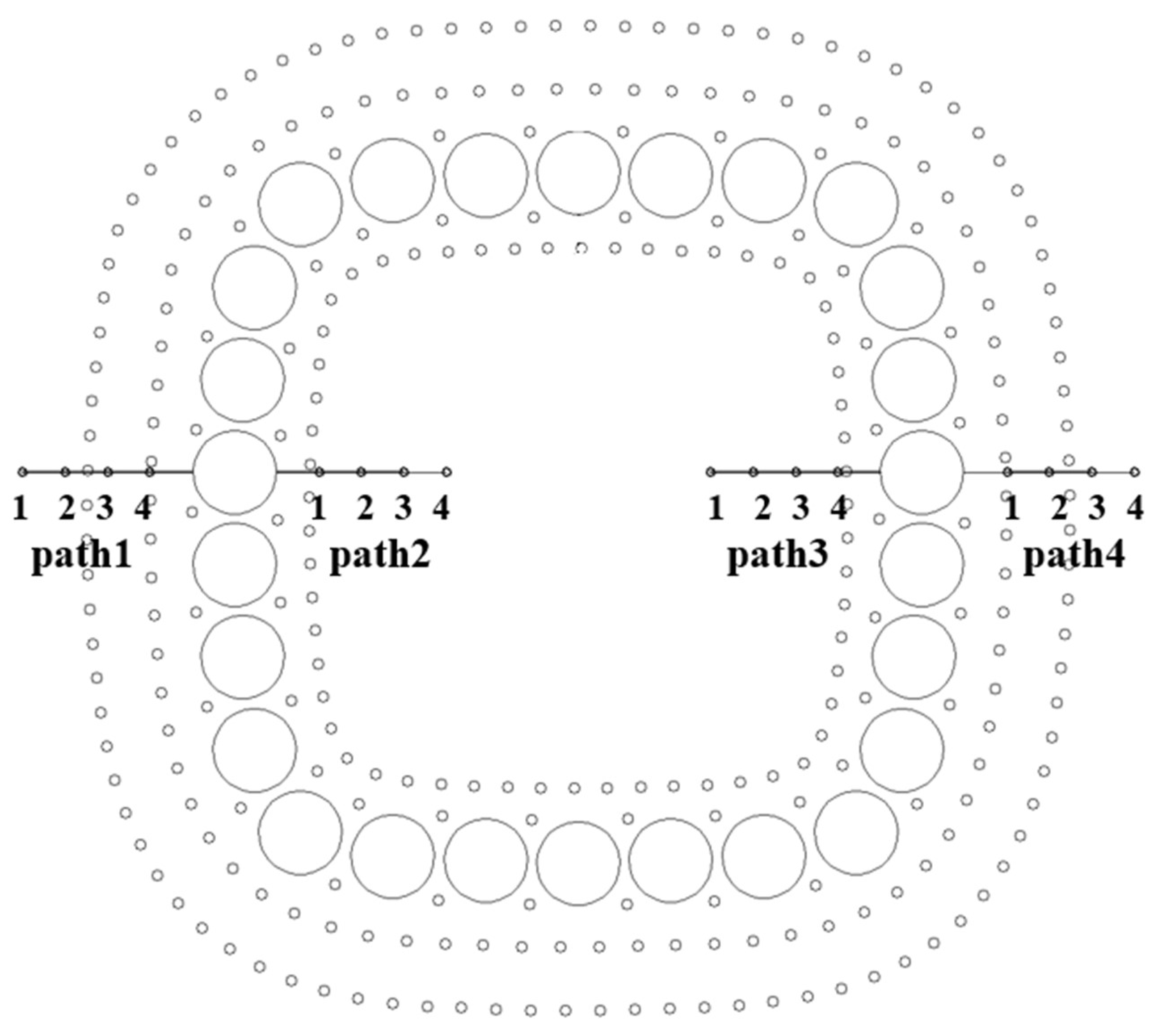
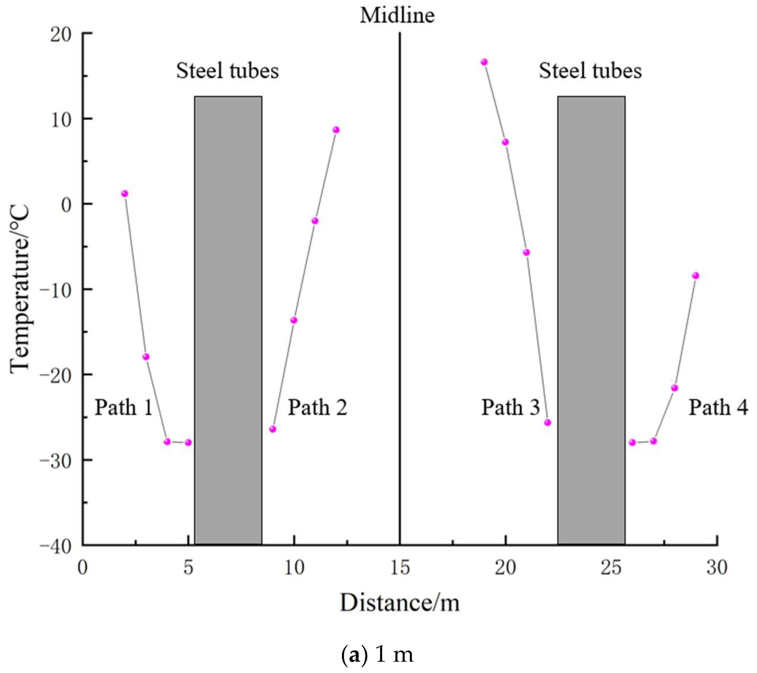
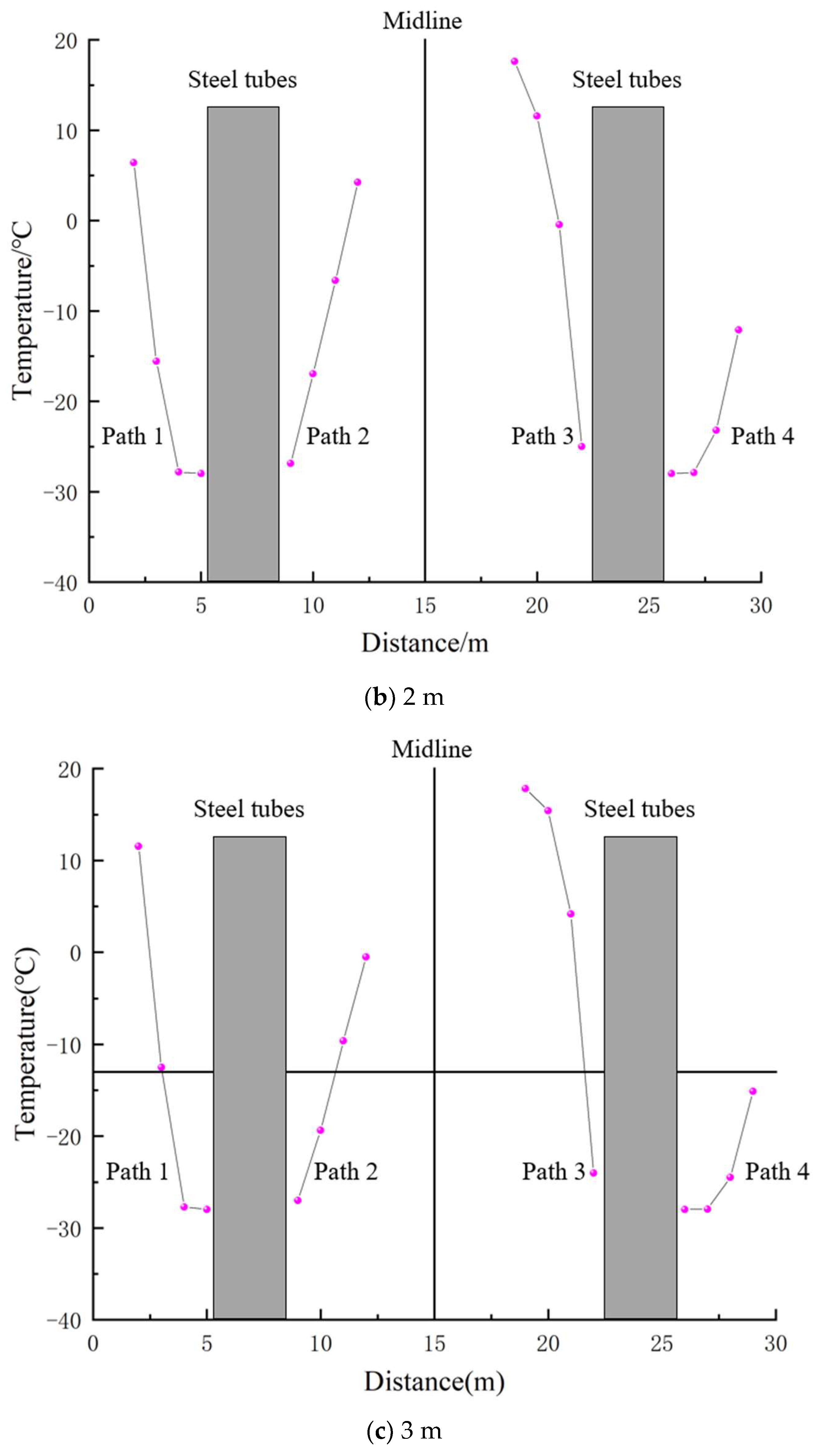
The YZ (X = 0) plane was chosen as the upstream of the head, and the YZ (X = 30) plane was chosen as the downstream of the head, both with a constant head; the other four faces of the model and the edge of the frozen pipe were set without flow for the adiabatic impermeable boundary. The boundary conditions are shown in Figure 4.

3.6. Path Setting

To investigate the temperature field of the frozen wall formed around the steel tube after the end of freezing and the development of the temperature field along the seepage direction, six observation paths were set up in the numerical model. The first path was set on the left side of the steel tube in the upstream area, starting and ending at coordinates (1.9, 5, 16) and (4.9, 5, 16), with a total of four observation points set at 1 m intervals. The second path was set on the right side of the steel pipe in the upstream area, starting and stopping at coordinates (8.9, 5, 16) and (11.9, 5, 16), with a total of four observation points set at 1 m intervals. The third path was set inside the top steel tube, starting and stopping at coordinates (15, 5, 21) and (15, 5, 18), with four observation points set every 1 m. The fourth path was set at the top of the steel tube. The starting and stopping coordinates were (15, 5, 28) and (15, 5, 15), with four observation points are set every 1 m. The fifth path was set to the left of the steel pipe in the downstream region. The starting and stopping coordinates were (18, 5, 16) and (21, 5, 16), with four observation points are set every 1 m. The sixth path was set on the right side of the steel tube in the downstream area, starting and stopping at coordinates (25, 5, 16) and (28, 5, 16), with a total of four observation points per 1 m. The observation path and observation points are shown in Figure 5.

4. Analysis of Calculation Results

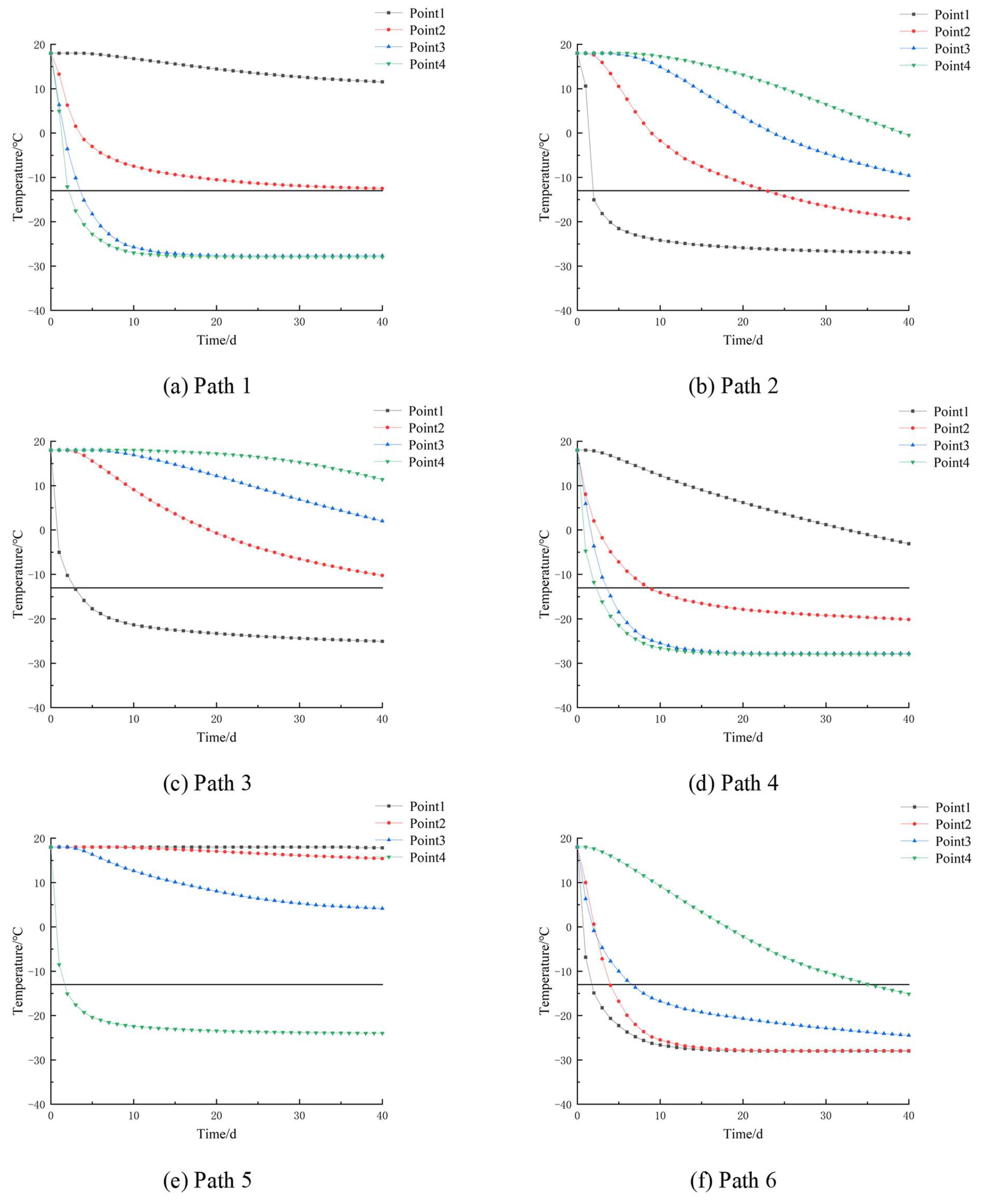
4.1. Analysis of Freezing Temperature Field

To analyze the development of the temperature field of the tube–curtain freezing method under different heads of water, the development of the temperature field at freezing times of 1 day, 2 days, 4 days, 6 days, 15 days, and 30 days was selected for analysis, as shown in Figure 6. From the diagram, it can be observed that the freezing wall formed by the same row of freezing pipes began to circle on day 2. On day 4, the frozen walls formed by two adjacent rows of freezing pipes began to circle. On day 6, a complete freezing wall formed around the pipes. The freezing wall formed on day 30 met the construction requirements, but it also needed to be maintained to ensure the stability of the freezing wall. Moreover, 15 days before freezing, the temperature field was less affected by the seepage effect, and the development of the frozen curtain was the same, whereas, 30 days after freezing, the development of the frozen curtain presented an asymmetric state, with seepage rate asymmetry becoming more obvious. The development of the freezing temperature field at different heads of water after active freezing was very different, as shown in Figure 7. Due to the effect of seepage, the thickness of the upstream freezing wall decreased with the increase in seepage velocity. The thickness of the downstream freezing wall increased with the increase in seepage velocity. The asymmetry of the curtain of permafrost increased with the rate of seepage.

The relationship between the head of water and the upstream and downstream freezing walls was obtained by measuring the distance from the steel pipe to the outer ring of the −13 °C permafrost curtain, as shown in Figure 8. From Figure 8, it can be seen that the seepage velocity was inversely proportional to the thickness of the upstream frozen curtain and positively proportional to the thickness of the downstream frozen curtain. To further verify the effect of seepage action on the development of the temperature field of the permafrost curtain, the analysis of frozen paths 1, 2, 5, and 6 of permafrost curtain at 40 days under different heads of water was carried out, and the temperature spatial distribution curve was plotted, as shown in Figure 9. According to Figure 9, the temperature at the upstream observation point increased with the increase in head of water, and the diffusion of cold in the upstream freezing tube was inhibited by seepage; the temperature at the downstream observation point decreased with the increase in head of water, and the seepage promoted the diffusion of cold in the freezing pipes.

Without the seepage flow, the temperature spatial distribution curve was symmetrical about the center line. Under the influence of seepage flow, the temperature spatial distribution was inclined downstream. The above analysis allowed concluding that a larger head of water resulted in a more obvious effect of seepage on the temperature field. Hence, the working condition with a head of water of 3 m was selected here for the path analysis. The temperature variation curves of each observation point on different paths over time are shown in Figure 10. The points on path 1 and path 6 correspond to symmetrical positions on the outside of the steel tubes at the upstream and downstream, as shown in Figure 10a,f. Only two observation points on path 1 reached temperatures below −13 °C after freezing, and the lowest temperature of observation point 4 was about −27.9 °C. The temperature at all four observation points on path 6 dropped below −13 °C, and the lowest temperature at observation point 4 is about 27.9 °C. Each point of path 2 and path 5 corresponded to the symmetrical position at the inner side of the upstream and downstream steel pipe, respectively, as shown in Figure 10b,e. After the end of freezing, the temperature of the two observation points on path 2 reached below −13 °C with a minimum temperature of about 26.9 °C, and the temperature of only one observation point on path 5 decreased below −13 °C with a minimum temperature of −24.6 °C. The cooling effect of the observation point close to the freezing pipes shows that the initial temperature dropped sharply; after reaching a certain temperature, the temperature stabilized until the end of freezing. It was found that the pore water resulted in the cooling of the upstream freezing pipes downstream due to the effect of seepage. The asymmetry of the curtain of frozen soil still occurred when the freezing pipes were arranged in the same way, but the minimum temperature was the same. Figure 10c,d shows the temperature variation curves over time for path 3 and path 4 on the inside and outside of the steel tube at the top of the model, respectively. There were only two rows of frozen tubes on the inside of the steel tube; thus, the temperature dropped below −13 °C at only one observation point on path 3, at about −25 °C. There were three rows of freezing tubes on the outside of the steel pipe; thus, there were three observation points on path 4 where the temperature dropped below −13 °C, and the lowest temperature was −27.9 °C. It can be seen that the seepage effect had less influence on the freezing effect when the seepage direction was horizontal to the freezing tube row direction.

4.2. Analysis of Forced Thawing Temperature Field

As the ground undergoes frost heaving and thaw collapsing during the thawing process, grouting is generally used in the project to limit the ground settlement. Therefore, to guide the temperature field during the thawing and grouting process, a detailed analysis of the natural and forced thawing temperature field is needed to investigate which method is more suitable. Natural thawing refers to stopping the delivery of low-temperature brine to the freezing pipe after freezing, which results in the frozen soil curtain warming up to 0 °C under natural conditions. However, it was found that the temperature in most areas was below 0 °C after natural thawing for 270 days, and the time was too long to meet the construction requirements. Therefore, three kinds of forced thawing schemes were adopted, and hot brine of 5 °C, 20 °C, and 50 °C was fed into the freezing tube after active freezing. The thawing schemes are shown in

Table 3. Thawing program.

Thawing Program	1	2	3
Thawing Temperature	5 °C	20 °C	50 °C

. In the process of thawing, 0 °C was assumed to be the cutoff line for the complete thawing of frozen soil.

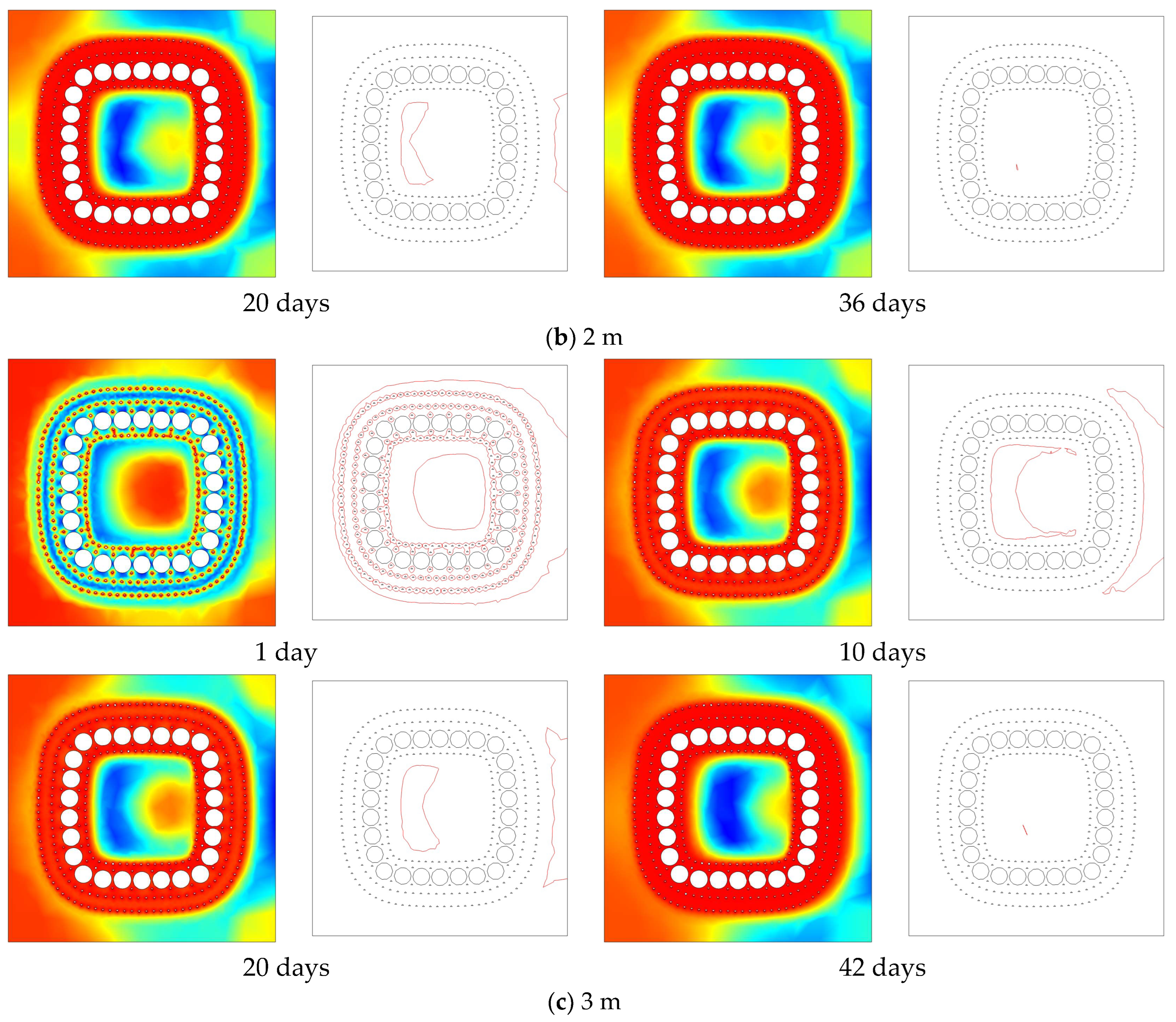
4.2.1. Development of Forced Thaw Temperature Field

To study the influence of seepage on the development of the temperature field in the process of forced thawing of a new tube–curtain freezing method, the thawing temperature was selected as option 2; the program of forced thawing temperature field development and the 0 °C isotherm diagram were simulated under different seepage velocities, as shown in Figure 11. According to Figure 11, the development pattern of the thawing temperature field was roughly similar for different heads of water. On the first day of thawing, the 0 °C isotherms were mainly distributed around the freezing pipe. On the 10th day, the frozen curtain melted in a large area, and the areas below 0 °C were mainly distributed in the center and downstream of the model. On the 20th day, the melting area continued to expand, and the area below 0 °C existed in the center and downstream of the soil, gradually expanding with time until the complete thawing. From the thawing temperature program, we can also observe that the downstream area experienced a temperature decrease during the thawing process, since the thawing of the permafrost curtain needed to absorb heat to lower the surrounding temperature; the low temperature was carried to the downstream area by the pore water under the influence of seepage, resulting in a downstream temperature decrease.

4.2.2. Comparison of Different Thawing Solutions

To study the development of temperature fields upstream and downstream of the three thawing scenarios under different heads of water, the development patterns of temperature fields at each observation point of path 1 and path 6 were analyzed for 30 days of thawing, as shown in Figure 12. Figure 12a shows the temperature change curves of each observation point of path 1 under three heads of water when the forced thawing temperature was 5 °C. Observation point 1 was the farthest from the heating tube and had the highest initial temperature; thus, the temperature change was the smallest, increasing by 5.11 °C, 4.07 °C, and 3.68 °C after 30 days of thawing under the three heads of water. Observation point 4 was the closest to the thawing pipe, with the lowest initial temperature and the largest temperature change; the temperature increased by 32.96 °C, 33.02 °C, and 33.07 °C after 30 days of thawing under the three heads of water. Figure 12b shows the temperature change curve of each observation point of path 6 under the three heads of water when the forced thawing temperature was 5 °C. In contrast to path 1, observation point 1 of this path was closest to the heating tube and had the lowest initial temperature and the largest temperature change; the temperature increased by 32.98 °C, 32.99 °C, and 33 °C after 30 days of thawing under the three heads of water. Observation point 4 was the farthest away from the thawing tube and had the highest initial temperature with the smallest temperature change; the temperature increased by 9.56 °C, 12.82 °C, and 16.67 °C after 30 days of thawing under the three heads of water. Similarly, by analyzing Figure 12c–f, we could obtain the temperature change of each observation point when the forced thawing temperature was 20 °C and 50 °C. In addition, it was found from Figure 12 that the temperature increased quickly and the thawing efficiency was higher at the observation points closer to the heating tube in the early stage of thawing; therefore, the thawing settlement displacement was larger at the early stage of thawing. Accordingly, it is necessary to carry out anti-thawing intervention as early as possible to avoid the influence of excessive thawing displacement on the structure.

To study the effect of different heads of water and forced thawing temperature on thawing time, a series of simulated experiments were carried out. The thawing temperature and thawing time are shown in

Table 4. The time required for complete thawing at different temperatures for different heads of water.

		Temperature	5 °C	20 °C	50 °C
	Time (Days)
Heads of Water
1 m			39	25	20
2 m			61	37	27
3 m			82	42	31

. It can be found from the table that the thawing temperature and thaw time were inversely proportional when the head difference was consistent (the higher the thawing temperature, the shorter the thaw time). When the thawing temperature was consistent, the head difference was proportional to the thaw time (the greater the head difference, the longer the thaw time).

5. Conclusions

This paper analyzed the application of a new pipe curtain freezing method in estuary construction, discussed the effect of seepage action on the freezing and thawing temperature fields, and obtained the following conclusions:

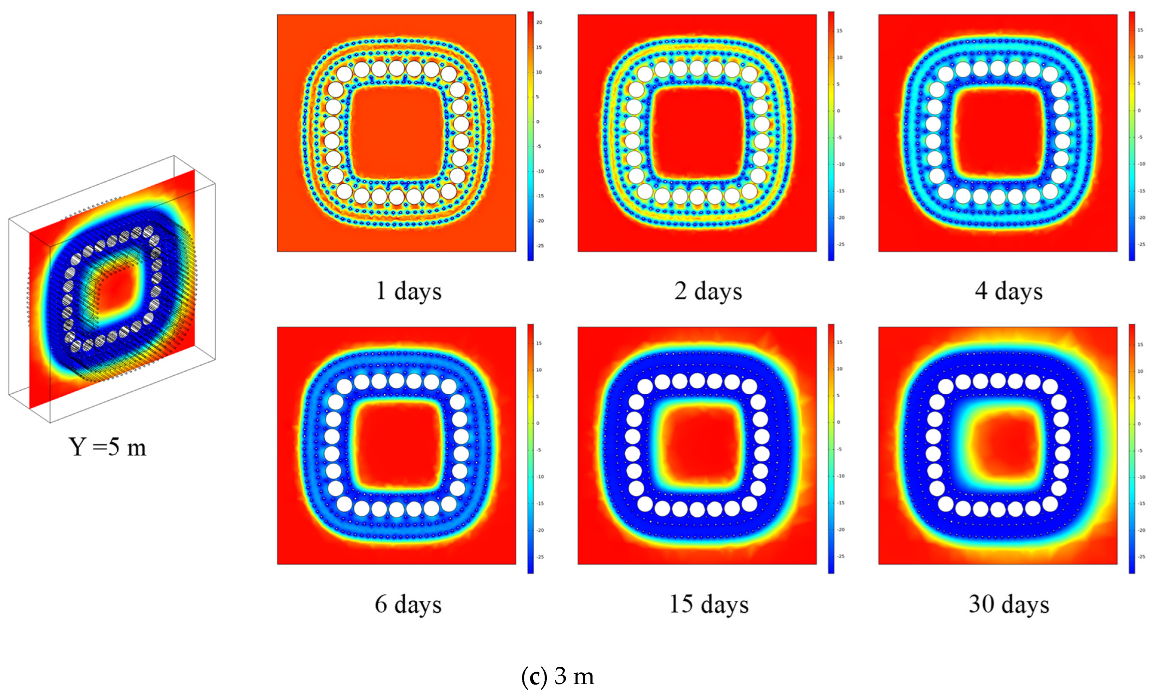
• During the active freezing period, the frozen curtain formed by the same row of frozen pipes started to cross circles after 2 days of freezing, the frozen curtain formed by different rows of frozen pipes started to cross circles after 4 days of freezing, and a more complete frozen wall started to form after 6 days of freezing, at which time the development of the frozen curtain was not significantly affected by the seepage. The frozen curtain formed after 30 days of freezing met the construction requirements. To ensure safe construction, the curtain must be maintained frozen; hence, it needs to freeze 40 days before construction can be carried out.
• During active freezing, the seepage action has a greater impact on the development of the permafrost curtain. The seepage action carries the cold energy generated by the upstream freezing tube to the downstream; therefore, there is a phenomenon of thin permafrost curtain upstream and thick permafrost curtain downstream, which becomes more evident with the increase in seepage velocity.
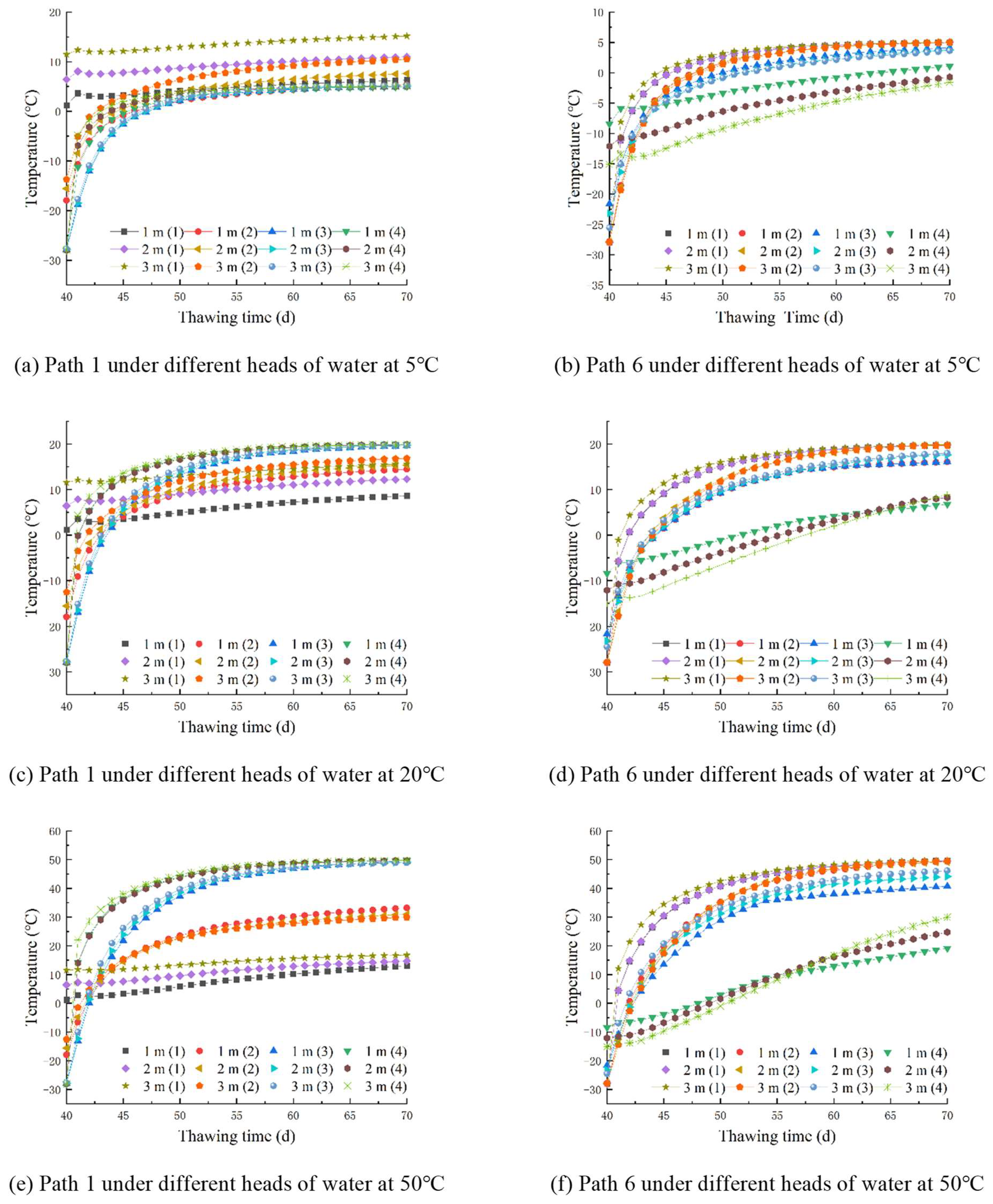
• During the forced thawing process, larger heads of water lead to a more obvious change in time required to raise the thawing temperature to completely thaw. For example, when the head difference was 3 m, it took 82 days to completely thaw at a thawing temperature of 5 °C, and only 31 days to completely thaw at a thawing temperature of 50 °C; when the head difference was 1 m, it took 39 days to completely thaw at a thawing temperature of 5 °C, and 20 days to completely thaw at a thawing temperature of 50 °C.
• The thawing effect is good at the beginning of thawing with the high warming rate of permafrost curtain, whereby about 90% of the permafrost curtain could be thawed in 15 days, and the temperature change of permafrost curtain tended to be flat after 15 days. The study of different heads of water and different forced thawing temperatures found that larger heads of water resulted in a longer thawing time. At the same thawing temperature, the thawing time for a 3 m head of water was about two times that for a 1 m head of water is 1 m. A higher thawing temperature resulted in a shorter the thawing time. At the same head of water, the thawing time at a temperature of 50 °C was about 0.5 times that at a temperature of 5 °C.
• The new tube–curtain freezing method is suitable for the construction of the estuary channel; due to the special nature of its freezing tube and steel pipe arrangement, a permafrost curtain with good waterproofing and high strength can be formed by actively freezing for 40 days, providing security for construction excavation. Jacking into the steel pipe can avoid the problem of thawing soil subsidence of the frozen curtain at the end of construction. Due to the large volume of the formed frozen curtain, in order to accelerate the construction progress, forced thawing of the frozen curtain can be performed by sending high-temperature brine to the frozen pipes to speed up the thawing of the frozen curtain.
• The use of the freezing method for underground construction is more environmentally friendly, with no pollution to the surrounding environment, no foreign substances into the soil, and less noise. Furthermore, the freezing curtain will melt away after the freezing is over, without affecting the underground structure around the building. Conveniently, it can effectively shorten the construction period, thus reducing the construction cost. It is highly adaptable and can be used for reinforcement of any water-bearing strata under various complex geological and hydrogeological conditions, and it is basically independent of the form, plan size, and depth of the pit. Its application is in line with the concept of sustainable development.

Due to the idealized characteristics of numerical simulations, which are very different from the complexity of actual engineering, the conclusions obtained do not necessarily coincide with actual engineering, and there are many limitations to the conclusions. Therefore, they can only be used as a reference before construction to provide theoretical guidance for development; the construction process still needs to be explored according to engineering reality.

References

1. Zhang, C.; Yang, W.H.; Qi, J.G. Analytic computation on the forcible thawing temperature field formed b-y a single heat transfer pipe with unsteady outer surface temperature. J. Coal Sci. Eng. 2015, 18, 8–24. [Google Scholar]
2. Ma, W. Review and prospect of the studies of ground freezing technology in China. J. Glaciol. Geocryol. 2001, 23, 218–224. [Google Scholar]
3. Yue, F.T.; Qiu, P.Y.; Yang, G.X. Numerical calculation of the freezing method for the contact channel of the cross-river tunnel. J. Coal 2005, 30, 710–714. [Google Scholar]
4. Hu, K.; Zhou, G.Q.; Li, X.J. Law of Soil Frost Expansion under Different Constraints. Int. J. Coal Geol. 2011, 36, 1653–1658. [Google Scholar]
5. Andersland, O.B.; Ladanyi, B. Frozen Ground Engineering; Wiley: Hoboken, NJ, USA, 2004. [Google Scholar]
6. Li, W.Q. Research and Application of Tube Curtain Method in Environmental Protection. Int. J. Constr. Constr. 2003, 33, 229–231. [Google Scholar]
7. Huang, F.; Shi, R.J.; Yue, F.T. Model Test of the Boundary Development Process of the Frozen Wall of Steel Tube Permafrost Co-Structure. J. Rock Mech. Eng. 2022, 41, 3063–3072. [Google Scholar]
8. Yuan, Y.H.; Yang, P. Application of Artificial Freezing Technology in Mine Tunnel. J. Railw. Eng. 2016, 33, 82–86+103. [Google Scholar]
9. Wang, L.; Chen, X.S.; Wu, J. Experimental study on the freezing law model of large underground space pipe curtain in urban water-rich strata. Tunn. Constr. Chin. Engl. 2022, 42, 1871–1878. [Google Scholar]
10. Liu, J.; Ma, B.; Cheng, Y. Design of the Gongbei tunnel using a very large cross-section pipe-roof and soil freezing method. Tunn. Undergr. Space Technol. 2018, 72, 28–40. [Google Scholar] [CrossRef]
11. Zhou, X.; Pan, J.; Liu, Y. Analysis of Ground Movement during Large-Scale Pipe Roof Installation and Artificial Ground Freezing of Gongbei Tunnel. Adv. Civ. Eng. 2021, 2021, 8891600. [Google Scholar] [CrossRef]
12. Hu, X.; Deng, S.; Ren, H. In situ test study on freezing scheme of freeze-sealing pipe roof applied to the Gongbei tunnel in the Hong Kong-Zhuhai-Macau bridge. J. Appl. Sci. 2016, 7, 27. [Google Scholar] [CrossRef] [Green Version]
13. Duan, Y.R.; Cheng, C.H. Experimental and Numerical Investigation on Improved Design f-or Profiled Freezing-tube of FSPR. Processes 2020, 8, 992. [Google Scholar] [CrossRef]
14. Zhang, P.; Ma, B.S.; Zeng, C. Key techniques for the largest curved pipe jacking roof to date: A case study of Gongbei tunnel. Tunn. Undergr. Space Technol. 2016, 59, 134–145. [Google Scholar] [CrossRef]
15. Kang, Y.S.; Liu, Q.S.; Cheng, Y. Combined freeze-sealing and New Tubular Roof construction methods for seaside urban tunnel in soft ground. Tunn. Undergr. Space Technol. 2016, 58, 1–10. [Google Scholar]
16. Duan, Y.; Rong, C.X.; Cai, H.B. Experimental Study on Mechanical Properties of “Top Tube-Permafrost” Composite Structure in Tube-screen Frozen Tunnel. Geol. Explor. Coal Fields 2022, 1–12. [Google Scholar]
17. Duan, Y.; Rong, C.; Cheng, H. Freezing Temperature Field of FSPR under Different Pipe Configurations: A Case Study in Gongbei Tunnel, China. Adv. Civ. Eng. 2021, 2021, 9958165. [Google Scholar]
18. Zhang, P.; Xu, P.; Yao, Q.; Zhang, Y.M.; Wang, T.; Zheng, Y.X. Construction technology of new pipe curtain method for subway stations with soft water-rich strata. Constr. Technol. Chin. Engl. 2022, 51, 35–39+53. [Google Scholar]
19. Zhou, W.; Hu, J.; Zeng, H.; Li, K.; Zeng, D.; Wang, Z.; Feng, J. Influence of different seepage velocities on the temperature field of the new tube screen freezing method. J. Hainan Univ. Nat. Sci. Ed. 2023, 41, 85–94. [Google Scholar] [CrossRef]
20. Zhou, Y.; Hu, J.; Xiong, H.; Ren, J.; Zhan, J.; Wang, Z. Temperature field analysis of the new pipe curtain freezing method in riverbank seepage control reinforcement. Coalf. Geol. Explor. 2022, 50, 110–117. [Google Scholar]
21. Duan, Y. Study on the Formation Law of Freezing Temperature Field of Tunnel Pipe Curtain and Its Mechanical Characteristics; Anhui University of Technology: Anhui, China, 2021. [Google Scholar] [CrossRef]
22. Duan, Y.; Rong, C.; Cheng, H.; Cai, H.; Xie, D.; Ding, Y. Model test of freezing temperature field of pipe curtain with different pipe jacking combinations. Glacial Permafr. 2020, 42, 479–490. [Google Scholar]
23. Han, X.M.; Xiao, M.Q.; Li, W.J.; Zhu, Y.Q. Study on Influence of Tube Curtain-Structure Mass Pipe Overhead on Station Floor and Stock Road Settlement. Tunn. Constr. 2020, 40, 170–178. [Google Scholar]
24. Zhang, S.L.; Wang, L.; He, Y.L.; Li, J.P.; Li, B. Study on Development of Freezing Temperature Field in Composite Stratigraphic Contact Channel. Undergr. Space Eng. J. 2022, 18, 266–273. [Google Scholar]
25. Li, Y.P. Characterization of Freezing Temperature Field Distribution in Combined Pipe Curtain Frozen Soil Structures; China University of Mining and Technology: Xuzhou, China, 2022. [Google Scholar] [CrossRef]
26. Abdelzaher, M.A.; Shehata, N. Hydration and synergistic features of nanosilica-blended high alkaline white cement pastes composites. Appl. Nanosci. 2022, 12, 1731–1746. [Google Scholar]
27. Owaid, K.A.; Hamdoon, A.A.; Matti, R.R.; Saleh, M.Y.; Abdelzaher, M.A. Waste Polymer and Lubricating Oil Used as Asphalt Rheological Modifiers. Materials 2022, 15, 3744. [Google Scholar] [CrossRef]
28. Ren, J.X.; Jia, L.; Yang, J.X.; Hu, J.; Lin, X.Q.; Zeng, D.L. Numerical simulation of the effect of groundwater salinity on the freezing temperature field at the bottom of foundation pits under seepage conditions. J. Changjiang Acad. Sci. 2023, 1–11. [Google Scholar]
29. Pimentel, E.; Papakonstantinou, S.; Anagnostou, G. Numerical interpretation of temperature distributions from three ground freezing applications in urban tunnelling. Turn Undergr. Space Technol. 2012, 28, 57–69. [Google Scholar] [CrossRef]
30. Yao, Z.; Cai, H.; Xue, W. Numerical simulation and measurement analysis of the temperature field of artificial freezing shaft sinking in Cretaceous strata. AIP Adv. 2019, 9, 025209. [Google Scholar] [CrossRef] [Green Version]
31. Zhao, Y.H.; Yang, P.; Wang, N.; Zhang, Y.W. Study on the thawing temperature field of MJS+ horizontal freezing reinforcement in the overlapping area of the underpass station. J. For. Eng. 2021, 6, 159–166. [Google Scholar]
32. Yan, Q.; Wu, W.; Zhong, H.; Zhao, Z.; Zhang, C. Temporal and spatial variation of temperature and displacement fields throughout cross-passage artificial ground freezing. Cold Reg. Sci. Technol. 2023, 209, 103817. [Google Scholar]
33. Qu, D.; Luo, Y.; Li, X. Study on the Stability of Rock Slope Under the Coupling of Stress Field. Seepage Field, Temperature Field and Chemical Field. Arab. J. Sci. Eng. 2020, 45, 8315–8329. [Google Scholar]
34. Wang, B.; Rong, C.; Lin, J. Study on the formation law of the freezing temperature field of freezing shaft sinking under the action of large-flow-rate groundwater. Adv. Mater. Sci. Eng. 2019, 2019, 1670820. [Google Scholar] [CrossRef] [Green Version]
Figure 1. Construction flowchart.
Sustainability 15 09367 g001
Figure 2. Preliminary design of tube–curtain structure.
Sustainability 15 09367 g002
Figure 3. Numerical model.
Sustainability 15 09367 g003
Figure 4. Schematic diagram of the boundary conditions.
Sustainability 15 09367 g004
Figure 5. Path layout.
Sustainability 15 09367 g005
Figure 6. The development of the temperature field during freezing process with different heads of water.
Sustainability 15 09367 g006aSustainability 15 09367 g006b
Figure 7. The development of the temperature field across 40 days of freezing with different heads of water.
Sustainability 15 09367 g007
Figure 8. The relationship between the head of water and the thickness of the frozen curtain.
Sustainability 15 09367 g008
Figure 9. Spatial distribution of freezing temperature over 40 days.
Sustainability 15 09367 g009aSustainability 15 09367 g009b
Figure 10. The curve of temperature change over time for each path of the freezing process.
Sustainability 15 09367 g010
Figure 11. Cloud and isothermal diagrams of the thaw temperature field at 20 °C.
Sustainability 15 09367 g011aSustainability 15 09367 g011b
Figure 12. Temperature variation curves of each point of path 1 and path 6 for different thawing schemes.
Sustainability 15 09367 g012