A System Optimization Approach for Trains’ Operation Plan with a Time Flexible Pricing Strategy for High-Speed Rail Corridors

Abstract

Optimizing the train plan for high-speed rail systems should consider both the passengers’ demands and enterprise’s benefits. The choice of the departure time period is the most important factor affecting the passenger demand distribution. In this paper, the optimization problem of a train operation plan based on time period preference is studied for a high-speed rail corridor. First, according to the travel process of the passengers, the extended service network for a high-speed rail system is established. The main factors that influence the passengers’ travel choices are analyzed, and the departure time period preference, stop time and flexible pricing strategy based on the time period preference are put forward. The generalized travel cost function, including the convenience, ticket fare and stop time costs, is constructed, and a two-level programming model is established based on the function. The upper-level planning model is formulated as a mixed 0–1 programming problem that aims at maximizing the revenue of the railway enterprise. It is mainly constrained by passenger travel demand and solved by improved genetic algorithms. The lower-level model is a user equilibrium (UE) model. The Frank–Wolfe algorithm is used to allocate multiple groups of OD (origin and destination) passenger flows to each train so that the generalized travel expenses of all the passengers with the same OD are minimized and equal. Finally, the train operation plan is solved based on the Lan-xi (Lanzhou–Xi’an) high-speed rail data, and the validity of both the model and algorithm is verified.

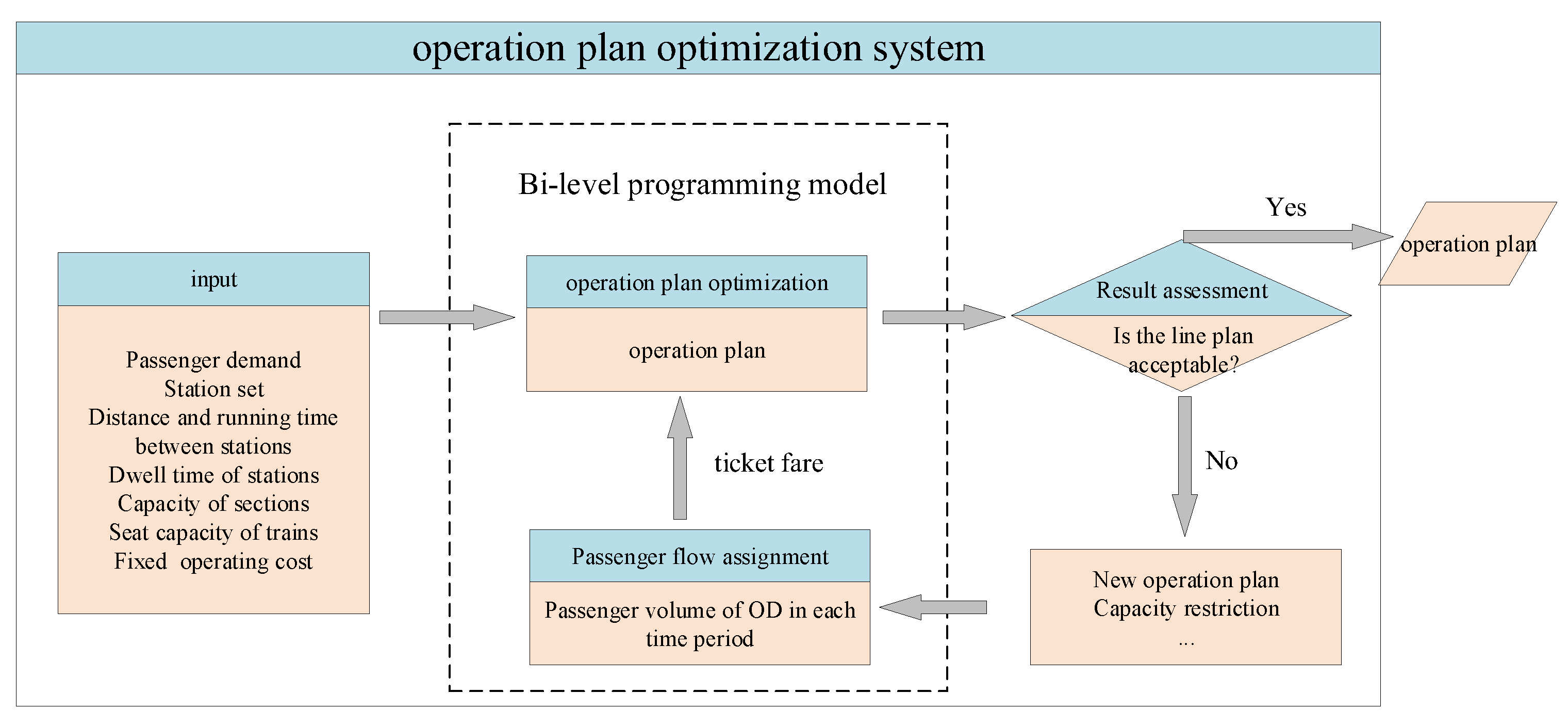
1. Introduction

As a new type of transportation mode, high-speed rail has changed people’s travel concept with its advantages of high efficiency and speed, so that the travel demand of passengers is not limited to the realization of displacement but takes into account comfort, time consumption and other factors. The introduction and development of high-speed rail provides travelers with a new travel choice [1]. The travel choice behavior of passengers helps us to understand their actual travel demand [2,3,4]. Zhang, P. et al. mentioned that current research on passenger travel behavior mainly considers the influence of attributes such as price and time of transportation mode on choice behavior [5]. The passengers’ travel choice behavior will be affected by personal travel habits, travel purpose, travel distance and other factors. Studying the passengers’ travel choice behavior can better explain the passenger’s actual travel demand, and since it is affected by personal travel habits, travel purposes, travel distances and other factors [6,7,8], it will lead to passengers’ preferences for different departure times. Mitropoulos, L. [9] mentioned that MaaS can provide passengers with information about their journeys, help them make better travel choices, improve the efficiency of the network by optimizing supply and demand and increase passenger satisfaction. Specifically, the passenger flow volume is unevenly distributed over time. Passengers need to refer to the high-speed rail operation plan (including the departure frequency, operation section, traveling time, stop plan, etc.). On the other hand, railway enterprises need to formulate a reasonable operation plan according to the travel demand of passengers, and they can also formulate management measures to rationally manage and control the passenger flow to improve the passengers’ travel satisfaction and benefits.

We offer the following three contributions to the optimization approach for an operation plan of high-speed rail:

• Applying flexible pricing to guide the passengers’ travel choices reasonably on high-speed rail is shown in Section 3.2.
• Bilevel programming is used to describe the dynamic feedback process of decision-making between the railway enterprise and passengers, and the improved genetic algorithm and Frank–Wolfe algorithm are used to realize the solution of the double-layer programming model, as shown in Section 4 and Section 5.
• Applying a multiple OD flow distribution in high-speed rail via the establishment of a high-speed rail service network is shown in Section 3.3 and Section 4.2.

The paper is organized as follows: Section 2 reviews the studies about the optimization of train operation plan and the flexible pricing strategy of high-speed railway. Section 3 establishes the extended service network of the high-speed rail system and constructs a generalized travel cost function. Section 4 establishes a two-level programming model based on a generalized travel cost function. Section 5 solves the upper-level planning model using an improved genetic algorithm and the lower-level planning model using the Frank–Wolfe algorithm. Section 6 verifies the validity of the model and algorithm based on data from Lanzhou West Station to Xi’an North Station. In Section 7, the conclusions are presented.

2. Literature Review

The ticket fare is the main component of the passenger’s generalized travel cost, and the fluctuation of the fare affects the passenger’s travel choice [10]. Gabor, M.R. mentioned that because airlines are customer-oriented, they provide an example of revenue management for other companies [11]. A flexible pricing strategy provides a new way for railway enterprises to better manage their operations. Since 2018, flexible pricing has been implemented on some rail lines in China, which has become an effective measure to guide passengers to change their travel choices, but there is not much research on the flexible pricing of high-speed rail. The railroad’s single pricing strategy has caused dramatic fluctuations in passenger flow and revenue difficulties. Qin, J. et al. [12] maximized ticket sale revenue with expected travel cost as the reference point and used prospect theory to construct a differentiated pricing model under elastic demand. Based on the benefits for railway enterprises, Z. Xiaoqiang et al. [13] proposed a dynamic pricing method for different customer groups. This method sets the ticket price of different grades of seats and limits the number of seats provided in each grade. The results show that in the off-season and peak season of passenger flow, different fares for different groups can improve the profit of railway enterprises. J.-S. Chou et al. [14] first constructed the space–time map of the stations along the high-speed rail through a GIS. Then, they set up a floating fare model considering the operating costs of high-speed rail, the perceived cost of passengers and the cost of space–time compression and put forward some suggestions for the existing high-speed rail fare. K. Sato and K. Sawaki [15], Z. Tang et al. [16] and X. Zhang et al. [17] studied the dynamic pricing model of high-speed rail in a competitive environment with various modes of transportation. The dynamic pricing strategy mainly considers the impact of the passenger flow sharing rates of other modes of transportation. The game theory method is used to solve for the dynamic fare of high-speed rail, which maximizes the benefit. Under the condition of flexible passenger demand, X. Zhang et al. [18] proposed a joint pricing strategy by considering the railway and passenger costs at the same time. J. Zheng and J. Liu [19] propose a fare optimization method based on revenue management theory. On the basis of hierarchical pricing, the model for optimizing the fare of each grade is also established to maximize the rail benefit. Jin, F. L. et al. constructed a set of Nested-logit (NL) models to analyze passengers’ preferences for different factors under various scenarios. Additionally, for fixed transportation capacity conditions, an optimization model is built to optimize the pricing among trains of common lines [20]. One of the main reasons for lower rail revenues and wasted train seats is the lack of precision in pricing and allocating fares to the dynamic needs of passengers. Yin, X. et al. used the sparse method to simulate passenger ticket demand during the pre-sale period, established a stochastic nonlinear programming mathematical model with the objective of maximizing train revenue, and validated a joint optimization scheme for ticket pricing and allocation considering dynamic demand to promote the sustainable development of train revenue and railroads [21].

The establishment of the above pricing model requires a long-time range of data and is greatly affected by passenger flow demand. Based on this situation, this paper will refine the time range of the study to one day. Considering the obvious difference in the passenger flow in each period of a day, the paper proposes a strategy of flexible pricing based on the passenger travel volume in different time periods, which would not be affected by the total passenger flow demand.

The travel choice of passengers will be affected by the train operation plan [22]. The problem of the passenger flow distribution under certain conditions of train operation plan/timetable determination is a subject that many scholars paid close attention to for a period of time. Zhou, W. et al. [23] used a potential category model to classify passengers’ demand and obtained the results of passenger flow allocation based on prospect theory, the Logit model and passenger flow transfer model, which mainly considered three factors of passengers’ choice of traveling trains: travel time, fare and departure time. A differential pricing and seat allocation model was constructed, and the model was solved using a simulated annealing algorithm. Y. Hamdouch et al. [24] proposed a new passenger flow equilibrium distribution model based on a timetable, in which the discomfort degree of standing and sitting passengers was distinguished, and the continuous average method was adopted to solve the model. W. Li and W. Zhu [25] proposed a dynamic simulation model of the passenger flow distribution based on the train delay, aiming at the running space–time diagram of trains and time-varying travel demands of passengers. The results show that this model has a good prediction effect on the train delay and passenger flow distribution. S. Sun and W. Y. Szeto [26] proposed a random user equilibrium model of fixed demand and proved that the proposed model had a unique solution and solved the problem of passenger flow distribution based on the average cost by using the self-adjusting average method. Q. Fu et al. [27] analyzed the passenger flow distribution model based on the frequency and timetable proposed so far in detail and compared these models from the aspects of the hypotheses and modeling methods to summarize their advantages and disadvantages. They proposed a future research direction based on the existing traffic distribution model. The aim of such research is mainly generalized to minimize the travel cost (travel time and ticket prices) of the passenger and maximize the benefits of travel; the main constraints are related to flow conservation, traffic restrictions, services segment flow and nonnegative flow constraints. The research also obtained suitable models for large-scale networks and can provide decision support for the network adjustment of the passenger flow distribution. A passenger train plan based on the passenger flow distribution problem should be built according to the train plan as well as the passengers’ choice behavior to determine the network impedance [28].

However, considering the passenger flow distribution problem based on the train operation plan studied, the one-way influence of the passenger travel affected only by the train operation plan as well as the fixed operation plan cannot better satisfy the time-varying travel needs of passengers. According to the passenger flow demand in time (different time periods) and space (different ODs), the development of an operation plan can promote the matching of the transport capacity and demand and optimize the operation management of rail transit [27].

Other scholars began to study the problem of optimizing the train operation plans/timetables based on the demand response. E. Barrena et al. [29] generalized the train timetable problem in the case of dynamic passenger flow demand and studied the design problem of the rapid rail transit (RRT) train timetable in the context of dynamic demand to minimize the average waiting time of passengers and applied the large-scale adaptive neighborhood search algorithm. The optimization of train schedules depends on the space–time distribution of passenger demand in high-speed rail operations. Zhou, W. et al. propose a regret value corresponding to the total cost based on multiple demand scenarios and construct a robust optimization model for high-speed railway train scenarios to minimize the maximum regret value [30]. H. Niu et al. [31] studied the scheduling optimization problem in the case of time-varying passenger flow demand and established a quadratic integer programming model with linear constraints for a given stop plan, aiming to minimize the total passenger waiting time. Based on the stop planning model, J. Qi et al. [32] proposed an optimization method that can comprehensively consider the passenger distribution, running area and stop planning and turn it into a dual-objective problem to minimize the total running time of empty seats and the total number of train stops. Since the previous problem of determining the timetables with the goal of maximizing passenger satisfaction cannot reflect the actual choice of passengers, T. Robenek et al. [33] proposed a timetable design problem centered on the passenger choice under elastic demand and solved it by using a simulated annealing algorithm in combination with the pricing scheme. P. Shang et al. [34] studied the subway timetable problem in a dynamic passenger flow demand environment, established a model for a single-line subway with the goal of minimizing the total travel time of passengers and designed the corresponding spatial branch and bound algorithm to solve the model. Most of these studies are based on a dynamic/static passenger arrival rate, while in fact, the passenger arrival rate is variable and difficult to obtain [35].

As seen from the studies above, the train’s operation plan will affect the passengers’ travel choices, and the passengers’ travel choice can be used as the basis for railway enterprises to optimize the operation plan [36]. When only considering the interests of the railway enterprises or passengers, single-layer planning can be used to optimize the operation plans or passenger flow distribution. If both the benefits of railway enterprises and the utility of passengers are taken into account, we need to make decisions on both the operation plans and passenger travel choices. Based on this, this paper establishes a bilevel programming model to describe the relationship between the railway enterprise and travelers. The upper-level model is based on the travel needs of the passengers in time and space and optimizes the operation plan to maximize the rail revenue. The lower-level model is based on the operation plan and aims to minimize the total generalized cost and equate the generalized cost of each passenger to solve the passenger flow distribution in time and space. The feedback information from the upper layer to the lower layer represents the new development plan. In the passenger flow distribution of the lower layer, the passengers will adapt to the new development plan and regain a balance. In fact, it is common for passengers to adjust their travel choices to adapt to a new timetable in public transport [37,38].

In a road traffic network, the passenger trips are distributed in each OD, and there are multiple routes between each OD. When the passenger flow allocated to the road network equalizes the travel costs of all routes among each OD, the road network reaches the UE equilibrium. The flow distribution of all the ODs in the road network is often used in urban road traffic network design research [39,40]. However, there are few studies on the application of multiple OD distributions in high-speed rail. The physical path of the same OD is unique in a high-speed rail corridor. Therefore, we established the extended service network of high-speed rail by dividing a physical path into multiple space–time paths in terms of time to allocate the passenger flow of multiple ODs.

3. Problem Analysis

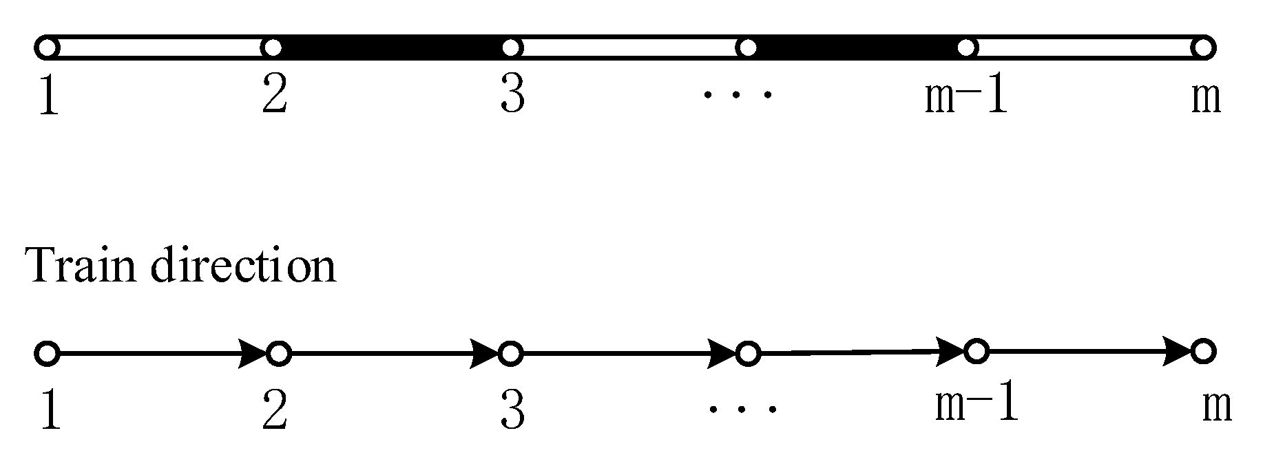
3.1. Related Assumptions and Notation

For the convenience of the research, this paper makes the following two assumptions:

• Passengers will not get off and transfer to a later train before arriving at the destination station once they take a certain train.
• In a given high-speed rail corridor, all trains have the same hardware parameters and leave at equal intervals within the same time period.
• Before moving further, we list the major notations in

  Table 1. Notation.

  Indexes
  $i,j,r,s$	indexes representing the nodes.
  $h,h^{\prime }$	indexes representing the time periods.
  $p$ $k$	index representing the parking plan at a node. index representing the trains.
  Sets
  $S$	the set of nodes.
  $W$	the set of ODs.
  $H$	the set of train operation time periods.
  $P$ $K_h$ $k_h$	the set of stop plans. the set of trains that depart from the initial station in time period $h$. the number of elements in $K_h$.
  $G_i^h$	the convenience cost of a departure from node $i$ in time period $h$.
  $T_{i,j}^{h,k}$	the in-node cost of taking train $k$ from node $i$ to node $j$ in time period $h$.
  $Y_{i,j}^{h,k}$	the in-train cost of taking train $k$ from node $i$ to node $j$ in time period $h$.
  Parameters
  $D$	the maximum number of trains per time period.
  $m$	the number of seats per train.
  ${\varphi }_{i,j}^p$	0–1 variable, it determines whether the train with a stop plan of $p$ is parked at both node $i$ and node $j$.
  $c^p$	the cost of running a train with a stop plan of $p$.
  $\alpha$ $\rho$	time value of passengers. adjustment factor.
  ${\beta }_i$	convenience factor of node $i$.
  $Q_{i,j}$	total passenger flow between node $i$ and node $j$ in one day.
  $U$	the maximum service capacity of the high-speed rail corridor in one time period.
  $\theta$	maximum train turnover rate.
  ${\eta }^{high}$	higher fare rate.
  ${\eta }^{low}$	lower fare rate.
  $L_{i,j}$	distance between node $i$ and node $j$.
  $t_{i,j}^{h,k}$	total stop time of the train $k$ from node $i$ to node $j$ in time period $h$.
  Decision variables
  $x_h^p$	the number of trains running with p-stop plans in time period $h$.
  $f_{i,j}^{h,k}$	the number of passengers in train $k$ from node $i$ to node $j$ in time period $h$.
  Auxiliary variables
  $y_{i,j}^h$	fare from node $i$ to node $j$ in time period $h$.
  $u_h$	total number of passengers traveling in time period $h$.
  ${\epsilon }_{i,i+1}^{h,k}$	0–1 variable that determines whether the train $k$ is parked at both node $i$ and node $i+1$ in time period $h$.
  $q_{i,i+1}^{h,k}$	the number of passengers on the train $k$ in the interval $\left(i,i+1\right)$ during time period $h$.
  $b_{h, i}^{h^{\prime },p}$	the number of trains arriving at node $i$ with stop plan $p$ departing from time period $h$ to time period $h^{\prime }$.

  .

3.2. Problem Description

As shown in Figure 1, given a high-speed rail corridor $\left(S,A\right)$, where $S$ represents the set of nodes, the train leaves from node one, passes through nodes $2,3,\cdot \cdot \cdot ,m-1$ and finally arrives at node $m$. $A$ is the set of intervals: an interval is the distance between two adjacent nodes. In this paper, the type of train is only dependent on the stop plan.

The passenger preference at different departure times during the operating hours of the day represents the degree to which passengers are attracted to travel at different times of the day. A high degree of time preference attracts more passenger traffic, resulting in most of the expected trips occurring during crowded time periods.

It not only impacts the passenger’s travel experience but also places more pressure on the operation of high-speed rail stations.

At present, the ticket fares for high-speed rail are only related to the mileage. The ticket fare of passengers with the same OD is the same. The generalized cost difference caused by passengers choosing different trains is only reflected in the convenience of different train departure times, so there will be a large variation in the passenger flow distribution in different time periods. We propose a pricing strategy based on the passenger flow during the time period by raising the ticket price and increasing the generalized cost of traveling during the crowded time periods to make the passengers transfer from the peak period to the low-peak period. The goal is to make the passenger flow in different periods tend to be balanced and reduce the station operating pressure while improving the satisfaction of passengers. At the same time, the railway enterprises need to develop the operation plan according to the new ticket fare and passenger flow allocation to adjust the number of trains to reduce the operation cost and maximize the benefits while meeting the demand of passenger flow.

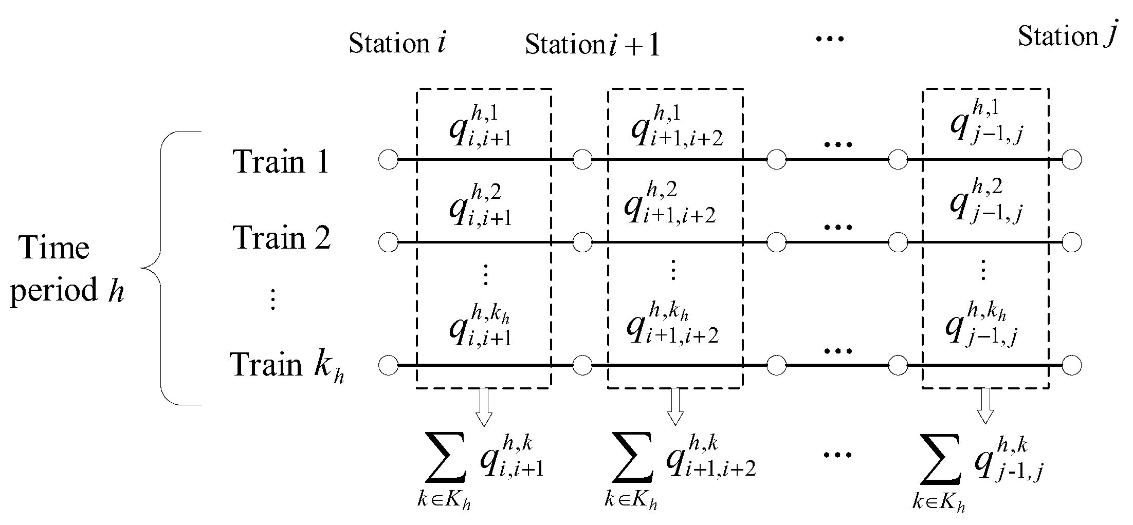
3.3. Passenger Travel Service Network

3.3.1. High-Speed Rail Service Network

Since the passenger’s travel choices will be affected by the above factors, it is difficult to reflect the actual travel situation in the simple physical network shown in Figure 1. To better describe the passenger travel choice behavior, we will construct the time and space network of the passengers’ departures and arrivals. Each node is expanded into an arc, and a high-speed rail service network, as shown in Figure 2, is constructed.

There are three trains in Figure 2. Train 1 and train 2 depart during the peak passenger flow period. Train 3 departs during the valley passenger flow period, and 0 indicates the virtual departure node of the passenger. The passenger travels by the departure arc, in-node arc and in-train arc.

3.3.2. Departure Arc

The process of passengers starting from the virtual node is called the departure arc. At this stage, the premise is that the passengers consider various factors when choosing whether it is convenient for their own travel. Therefore, in the departure arc, we need to evaluate the convenience of passengers traveling at each time. Taking into account the geographical location of each node, the economic level of the area and the average distance of the passengers arriving at the node, we define the travel ratio as a measure of convenience. We use $g_i^h$ to indicate the convenience of starting from the node during the time period. Since the degree of convenience is a dimensionless parameter, to facilitate the research, this will allow for the conversion of the cost function in terms of convenience. The higher the convenience is, the lower the convenience cost is for the passenger, and the higher the cost is. Equation (1) represents the convenience cost of a departure from node $i$ in time period $h$, $G_i^h$ is:

$$G_i^h=\frac{{\beta }_i}{g_i^h}, \forall h,i$$

(1)

where ${\beta }_i$ indicates that the convenience coefficient from node $i$ is only related to the departure site and can be obtained by an investigation and statistical analysis.

3.3.3. In-Node Arc

The process of parking a train at a node is called an in-node arc. In the hypothesis, we assume that the speed of the train is constant, so the difference in travel time for the OD passengers depends only on the stop time. This article only considers the extra time cost for the passengers. To quantitatively evaluate the impact of the stop time on passenger travel choices, we use the time value, $\alpha$, to convert the stop time, $t_{i,j}^{h,k}$, into a cost, $T_{i,j}^{h,k}$.

$$T_{i,j}^{h,k}=\alpha \cdot t_{i,j}^{h,k}, k\in K_h$$

(2)

where $t_{i,j}^{h,k}$ represents the stop time of the kth train from node $i$ to $j$ in time period $h$; $T_{i,j}^{h,k}$ represents the stop time cost of the kth train from node $i$ to node $j$ in time period $h$.

3.3.4. In-Train Arc

The running process of a train between adjacent nodes is called the in-train arc. The cost paid by the passenger during this process is the ticket fee, $y_{i,i+1}^h$. Considering the passenger’s comfort, the passenger experience will be affected by congestion on the train. The more crowded the train is, the more uncomfortable the passenger will be. Therefore, we use the adjustment factor, $\rho$, on the basis of the ticket fare, $y_{i,i+1}^h$, to represent the passenger’s comfort cost, $y_{i,i+1}^h\cdot \rho \cdot \frac{q_{i,i+1}^{h,k}}{m}$. Therefore, the total cost paid by the passenger on the in-train arc, $Y_{i,i+1}^{h,k}$ is:

$$Y_{i,i+1}^{h,k}\left(q\right)=y_{i,i+1}^h\cdot \left(1+\rho \cdot \frac{q_{i,i+1}^{h,k}}{m}\right)$$

(3)

3.3.5. Generalized Travel Costs

All the costs of the above three processes experienced by the passengers constitute the generalized travel costs.

$${\pi }_{i,j}^{h,k}=G_i^h+T_{i,j}^{h,k}+{\displaystyle \sum _{i\le s\le j-1}{\mathrm{Y}}_{s,s+1}^{h,k},} k\in K_h$$

(4)

In fact, the problem studied in this paper is to use differential pricing to balance the flow of each period to develop a train operation plan that can meet the passenger flow demand. In this way, the passenger’s generalized travel cost is minimized and equal in each time period, and the railway enterprises have the most benefit. Specifically, the train operation plan is developed by determining the number of trains for different types of stopping plans in each time period, and the trains are equally spaced in a certain order. Guided by the flexible fares, the operation plan and the travel options of the passengers can interact with each other. Therefore, this paper considers the establishment of a bilevel programming model to solve the problem. The upper-level planning model aims to maximize the benefit of railway enterprises. The lower-level planning model is based on the upper-level planning scheme. The passenger flow distribution is based on the minimum travel cost of the passengers. Figure 3 illustrates the process of optimizing the operation plan.

4. Construction of the Bilevel Programming Model

4.1. Upper-Level Planning Model

Each train has different travel costs due to the number of stops. $c^p$ indicates the cost of operating a train with stop plan, $p$. The number of trains with stop plan $p$ in time period $h$ is $x_h^p$. The rail enterprise daily cost is ${\displaystyle \sum _{p\in P}{\displaystyle \sum _{h\in H}{c}^p\cdot x_h^p}}$. For OD $\left(i,j\right)$, the fare for each time period and the passenger flow are $y_{i,j}^h$ and ${\displaystyle \sum _{k\in K_h}{f}_{i,j}^{h,k}}$, respectively. Therefore, the total income of the rail enterprise for one day is ${\displaystyle \sum _{\left(i,j\right)\in W}{\displaystyle \sum _{h\in H}{\displaystyle \sum _{k\in K_h}{f}_{i,j}^{h,k}\cdot y_{i,j}^h}}}$. With the goal of maximizing the revenue of the railway enterprise, the upper-level programming model objective function can be expressed as follows:

$$\max \left({\displaystyle \sum _{\left(i,j\right)\in W}{\displaystyle \sum _{h\in H}{\displaystyle \sum _{k\in K_h}{f}_{i,j}^{h,k}\cdot y_{i,j}^h}}}-{\displaystyle \sum _{p\in P}{\displaystyle \sum _{h\in H}{c}^p\cdot x_h^p}}\right)$$

(5)

• Departure capacity constraint

There is a limit on the number of trains departing from the node per unit time. The departure capacity constraint ensures that the total number of departures, ${\displaystyle \sum _{p\in P}{x}_h^p}$, from the originating node at any period, $h\in H$, does not exceed the starting capacity of the period, $D$. The constraint is expressed as follows:

$${\displaystyle \sum _{p\in P}{x}_h^p}\le D, \forall h\in H$$

(6)

• Passenger flow demand constraint

The passenger flow demand constraint ensures that the number of trains can satisfy the passenger flow demand at various time periods. According to a certain departure order and interval, it can be determined that the trains in the $h^{\prime }\left(h^{\prime }\in H\right)$ time period arrive at the nodes along the way. To simply and clearly describe which trains can reach the node during time period $h$, we set an auxiliary variable, $b_{h, i}^{h^{\prime },p}$, which indicates the number of trains with stop plan $p$ departing in time period $h^{\prime }$ and arriving at node $i$ in time period $h$. As shown in Figure 4, there are three trains with stop plan $p$ from station 1 in time period $h^{\prime }$, one of which arrives at station 2 during the time period $h$, and the remaining two trains arrive at node 3 during time period $h$. That is, $b_{h, 2}^{h^{\prime },p}=1$ and $b_{h, 3}^{h^{\prime },p}=2$.

where $b_{h, i}^{h^{\prime },p}$ satisfies Equation (7).

$${\displaystyle \sum _{h\in H}{b}_{h, i}^{h^{\prime },p}}=x_{h^{\prime }}^p$$

(7)

Therefore, the number of trains that can serve passengers from node $i$ to node $j$ during time period h is ${\displaystyle \sum _{h^{\prime }\in H}{b}_{h, i}^{h^{\prime },p}\cdot {\varphi }_{i,j}^p}$. Among them, ${\varphi }_{i,j}^p$ is a 0–1 variable. If the train with stop plan $p$ and stops at both node $i$ and node $j$, ${\varphi }_{i,j}^p=1$; otherwise, ${\varphi }_{i,j}^p=0$. Then, the number of seats available to passengers during the time period $h$ is ${\displaystyle \sum _{h^{\prime }\in H}{b}_{h,i}^{h^{\prime },p}\cdot {\varphi }_{i,j}^p\cdot m\cdot \theta }$ from node $i$ to node $j$, where $m$ is the total number of seats per train and $\theta$ is the maximum overload rate of a train.

Figure 5 shows the number of people in each section between node $i$ and node $j$ departing in time period $h$. $K_h$ is the train set from the originating station in time period $h$; $k_h$ is the number of elements in $K_h$, and $k_h$ can be calculated by Equation (8).

$$k_h={\displaystyle \sum _{p\in P}{x}_h^p}$$

(8)

To determine the maximum passenger flow of each interval between the station $i$ and the station $j$ during the time period $h$, we set the auxiliary variable $q_{i,i+1}^{h,k}$ to represent the number of passengers on the train $k$ in the interval $\left(i,i+1\right)$ in the time period $h$. $q_{i,i+1}^{h,k}$ satisfies Equation (9).

$${\displaystyle \sum _{r\le i, s\ge i+1}{f}_{r,s}^{h,k}}=q_{i,i+1}^{h,k}, k\in K_h$$

(9)

Therefore, the total number of passengers passing the interval $\left(i,i+1\right)$ during the time period $h$ can be expressed as ${\displaystyle \sum _{k\in K_h}{q}_{i,i+1}^{h,k}}$. The number of passengers carried by trains stopping at both node $i$ and node $j$ is ${\displaystyle \sum _{k\in K_h}{q}_{i,i+1}^{h,k}\cdot {\epsilon }_{i,i+1}^{h,k}}$, where ${\epsilon }_{i,i+1}^{h,k}$ is a 0–1 variable. If the train $k$ stops at both node $i$ and node $\left(i+1\right)$ in time period $h$, ${\epsilon }_{i,i+1}^{h,k}=1$; otherwise ${\epsilon }_{i,i+1}^{h,k}=0$. To ensure that passengers who want to depart from node $i$ to node $j$ in time period $h$ have an opportunity to take a train, the total number of seats must be greater than or equal to the total number of persons in each interval between node $i$ and node $j$ in time period $h$. Therefore, this constraint is represented as follows:

$${\displaystyle \sum _{p\in P}{\displaystyle \sum _{h^{\prime }\in H}{b}_{h,i}^{h^{\prime },p}\cdot {\varphi }_{i,j}^p\cdot m\cdot \theta }}\ge {\displaystyle \sum _{h\in H}{\displaystyle \sum _{k\in K_h}{q}_{s,s+1}^{h,k}\cdot {\epsilon }_{s,s+1}^{h,k},}} i\le s\le j-1$$

(10)

• Ticket fare constraints

Based on the wishes of the railway enterprise and passengers, we determine the upper limit, ${\eta }^{high}$, and lower limit, ${\eta }^{low}$, of the ticket fare rate. The corresponding fare for each OD $\left(i,j\right)\in W$ also has an upper limit, $y_{i,j}^{high}$, and a lower limit, $y_{i,j}^{low}$, which are calculated by Equations (11) and (12), respectively.

$$y_{i,j}^{high}=L_{i,j}\cdot {\eta }^{high}$$

(11)

$$y_{i,j}^{low}=L_{i,j}\cdot {\eta }^{low}$$

(12)

The ticket fare for any period, $h\in H$, depends on the total number of people traveling during this period, $u_h$. The formula for $u_h$ is as follows:

$$u_h={\displaystyle \sum _{\left(i,j\right)\in W}{\displaystyle \sum _{k\in K_h}{f}_{i,j}^{h,k}}}$$

(13)

Therefore, the ticket fare constraints can be expressed as follows:

$$y_{i,j}^h=y_{i,j}^{low}+\left(y_{i,j}^{high}-y_{i,j}^{low}\right)\cdot \frac{u_h}{U}$$

(14)

where $U$ is the service capacity of the high-speed rail line for a time period.

• Decision variable constraints

To ensure that the decision variables are nonnegative, the constraint is expressed as follows:

$$x_h^p\ge 0$$

(15)

4.2. Lower-Level Programming Model

In the lower programming model for the user equilibrium assignment, the passengers tend to choose the time period in which the travel cost is the smallest. The travel cost is an increasing function of the passenger flow during the period, and the passengers’ transfers in each period will change the travel cost of each path between the same OD. When the travel impedance of the passengers on any path between OD $\left(i,j\right)$ is equal, the UE equilibrium state is reached. The lower-level planning objective function is established with the goal of minimizing the total travel cost:

$$Z=\min \left(Z_1+Z_2+Z_3\right)$$

$$Z_1={\displaystyle \sum _{\left(i,j\right)\in W}{\displaystyle \sum _{i\le s\le j-1}{\displaystyle \sum _{h\in H}{\displaystyle \sum _{k\in K_h}{\displaystyle {\int }_0^{q_{s,s+1}^{h,k}}{Y}_{s,s+1}^{h,k}\left(\phi \right)d\phi }}}}}$$

$$Z_2={\displaystyle \sum _{\left(i,j\right)\in W}{\displaystyle \sum _{h\in H}{\displaystyle \sum _{k\in K_h}{G}_{i,j}^{h,k}}}}$$

$$Z_3={\displaystyle \sum _{\left(i,j\right)\in W}{\displaystyle \sum _{h\in H}{\displaystyle \sum _{k\in K_h}{T}_{i,j}^{h,k}}}}$$

• Passenger flow balance constraint

$${\displaystyle \sum _{r\le i,s\ge i+1}{f}_{r,s}^{h,k}}=q_{i,i+1}^{h,k}$$

(16)

• Demand constraint

The sum of the OD $\left(i,j\right)$ traffic on each train, $f_{i,j}^{h,k}$, is equal to the OD $\left(i,j\right)$ one-day traffic demand. The constraint is as follows:

$${\displaystyle \sum _{h\in H}{\displaystyle \sum _{k\in K_h}{f}_{i,j}^{h,k}}}=Q_{i,j}$$

(17)

• Decision variable constraint

To ensure that the decision variables are nonnegative, the constraint is expressed as follows:

$$f_{i,j}^{h,k}\ge 0, k\in K_h$$

(18)

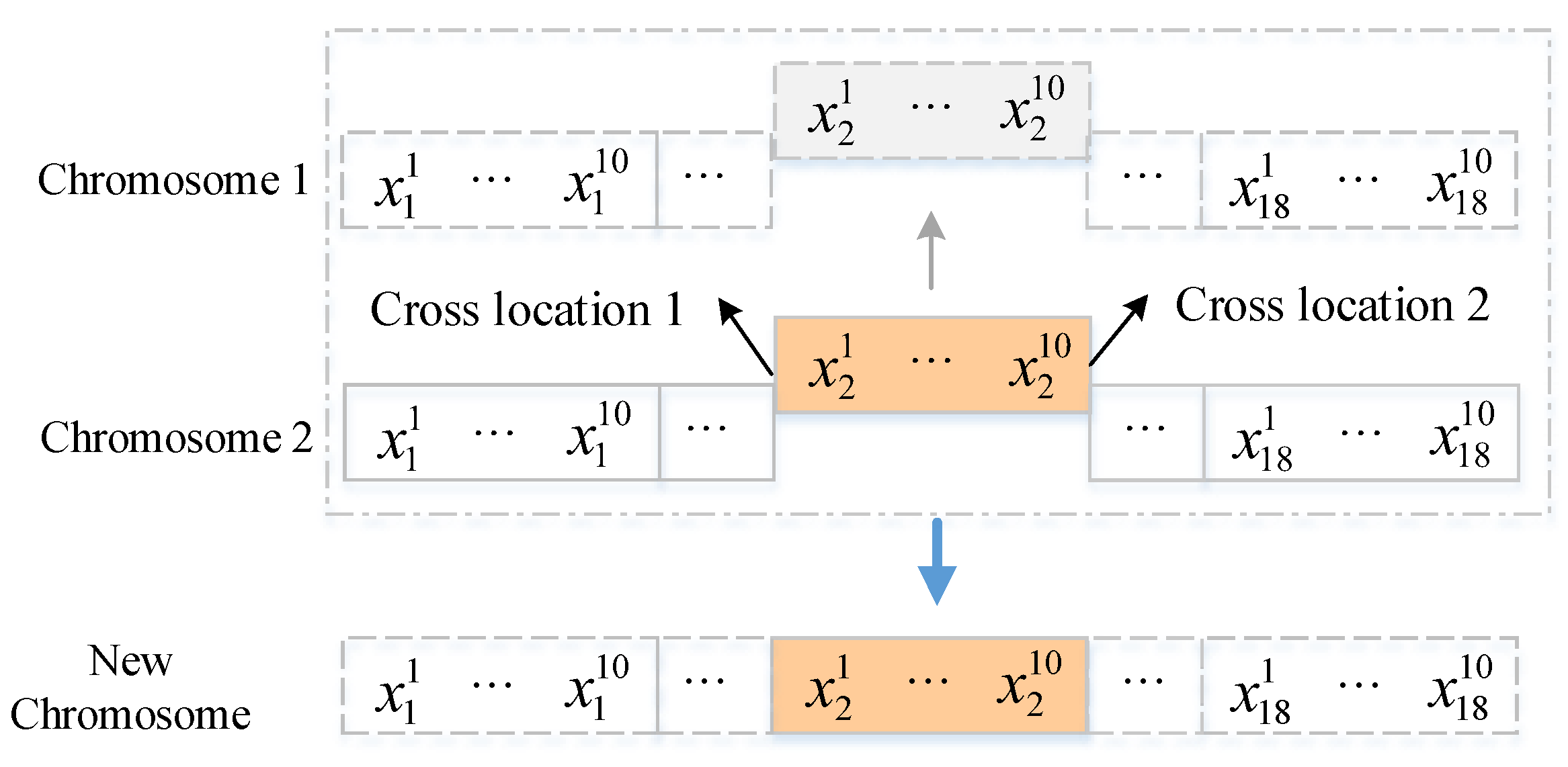
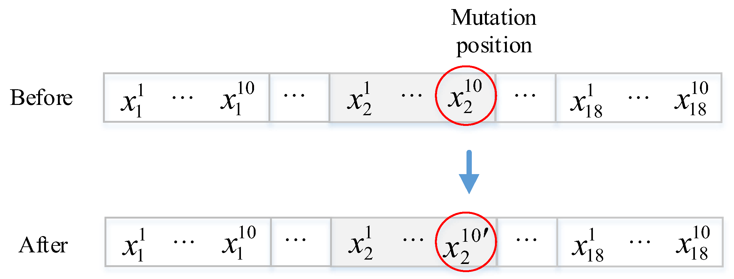
5. Solution Algorithm

5.1. Upper Layer Algorithm

Because the upper model is a nonconvex problem that cannot be solved by conventional optimization algorithms, a heuristic algorithm is considered. For practical engineering problems, the satisfactory solution obtained by an intelligent algorithm can also satisfy the requirements. Because of its strong global optimal solution ability and robustness, genetic algorithms often obtain better results than traditional algorithms in problems with a very complex search space. Therefore, we use a genetic algorithm to solve the upper-level programming model. The chromosomes are integer coded in the genetic algorithm of this paper, and each chromosome consists of 18 gene segments, representing 18 time periods in the day. Each gene fragment has 10 gene positions, which represent the number of trains with 10 stop plans. Therefore, a chromosome has a total of 180 gene positions, which are composed of 18 daily time periods and 10 stop plans, which can be expressed as the set $\left\{x_h^p\left|h\in H,p\in P\right.\right\}$.

Genetic algorithm solution process:

Step 1. Initialization.

Set the maximum genetic algebra to $Ge$, the probability of crossover to ${\vartheta }_{cor}$ and the probability of mutation to ${\vartheta }_{var}$. According to the above chromosomal coding rule in the upper layer and the search space corresponding to the constraints, the algorithm randomly generates an initial population of size $\sigma$. Set the number of iterations $\lambda =0$.

Step 2. Building a breeding pool.

For each individual of the current generation, the Frank–Wolfe algorithm is used to solve the lower-level planning model. Calculate the objective value of the upper-level objective function as an individual based on the results of the flow assignment and calculate the fitness, $F$, of each individual by using Equation (19). According to the degree of fitness, the individuals in the current population are sorted in descending order. The first half of the individuals with the highest fitness values are selected to enter the breeding pool.

$$F=\frac{R_{\max }-R}{R_{\max }-R_{\min }}$$

(19)

where $R$ is the target value of any individual in the current generation; $R_{\max }$ and $R_{\min }$ represent the maximum and minimum target values of the individuals in the current generation, respectively.

Step 3. Update the population with the elite retention strategy and adaptive mating rights strategy.

The selection operation is based on the individual fitness evaluation. Use a selection mechanism to select some individuals from the parent population to retain to the next generation. To ensure the convergence of the algorithm, this paper chooses the combined strategy of dynamic elite retention and adaptive mating rights.

The dynamic elite retention strategy consists of randomly selecting 10 individuals from the top ${\sigma }^{\prime }$ with the best fitness values in the parent population to replace ${\sigma }^{″}$ individuals with the worst fitness values in the present generation. This strategy can avoid having good individuals in the population being destroyed by the crossover and mutation operations, thus ensuring the convergence of the algorithm.

The adaptive mating rights strategy selects individuals from the mating pool for genetic operations. A selection probability, ${\omega }_a$, is set for each individual according to the individual fitness value in the mating pool. The higher the fitness value is, the greater the probability is that the individual will be selected. The individual selection probability is calculated as follows:

$${\omega }_a=F_a/{\displaystyle \sum _{a=1}^{\sigma /2}{F}_a ,} a=1,2\cdots \sigma /2$$

(20)

In this paper, we use double-point crossover; that is, after selecting the two chromosomes from the breeding pool, two different positions on one chromosome are randomly selected, and the gene fragment between the two positions is used to replace the corresponding gene fragment on the other chromosome. The crossover process is shown in Figure 6.

The mutation operation: a gene position on the chromosome is randomly selected for mutation, and let the value on the gene position randomly increase or decrease by 1 to produce a new chromosome. The mutation process is shown in Figure 7.

The Frank–Wolfe algorithm is used to solve the underlying plan for the new individuals. Check whether the new individual satisfies the upper constraint. If it is satisfied, transfer the new individual to the new population, set the number of individuals in the new population $\mu =\mu +1$ and go to step 4; if not, go to step 3.

Step 4: Determine the number of iterations.

Determine if $\mu$ equals $\sigma$; if no, go to step 3; if yes, set the iteration number, $\lambda =\lambda +1$. Continue to determine whether $\lambda$ is equal to the maximum genetic algebra, $Ge$; if not equal, then go to step 2; if equal, end the operation and output the largest target in the current generation and the corresponding target value.

5.2. Lower Layer Algorithm

The UE programming problem is a nonlinear convex programming problem; the objective function is strictly convex; the constraints are linear, and there is a unique solution corresponding to the UE condition. The Frank–Wolfe algorithm is a standard algorithm for solving problems with a convex objective function and linear constraints. Therefore, in this paper, we use the Frank–Wolfe algorithm to solve the lower UE planning problem.

The Frank–Wolfe algorithm solution procedure:

Step 1. Initialization.

Letting the time flow $u_h=0$, calculate the impedance, ${\pi }_{i,j}^h$. The passengers, $Q_{i,j}$, on each OD are loaded onto the train in an all-or-nothing manner, so that the passenger flow, $u_h^1$, of each time period of the first iteration is obtained. Set the iteration number as $n=1$.

Step 2. Update impedance.

Update the impedance, ${\pi }_{i,j}^{h,n}$, according to Equations (13) and (3).

$${\pi }_{i,j}^{h,n}={\pi }_{i,j}^h\left(u_h^n\right)$$

(21)

Step 3. Find the iteration direction.

According to the updated impedance, the passengers, $Q_{i,j}$, on each OD are loaded onto the train in an all-or-nothing manner again, so that the passenger flow, $u_h^1$, of each time period of the first iteration is obtained.

Step 4. Calculate the iteration step size.

Solve the minimum value problem:

$$\min {\displaystyle \sum _{\left(i,j\right)\in W}{\displaystyle \sum _{h\in H}{\displaystyle {\int }_0^{u_h^n+{\gamma }_n\left(v_h^n-u_h^n\right)}{\pi }_{i,j}^h\left(\phi \right)d\phi }}}$$

(22)

Let the solution be denoted as ${\gamma }_n$.

Step 5. Update the passenger flow, $u_h^{n+1}$, for each time period.

$$u_h^{n+1}=u_h^n+{\gamma }_n\left(v_h^n-u_h^n\right)$$

(23)

Step 6. Discriminant convergence.

When the change rate of the objective function value of two consecutive iterations is less than a predetermined decimal number, stop the iterative operation. Otherwise, set the iteration number, $n=n+1$, and go to step 1. In this paper, Equation (24) measures the degree of convergence of the iteration, where $\tau$ is our given threshold.

$$\sqrt{{\displaystyle \sum _{h\in H}{\left(u_h^{n+1}-u_h^n\right)}^2}}/{\displaystyle \sum _{h\in H}{u}_h^n}\le \tau$$

(24)

The genetic algorithm flow chart is shown in Figure 8.

6. Numerical Experiment

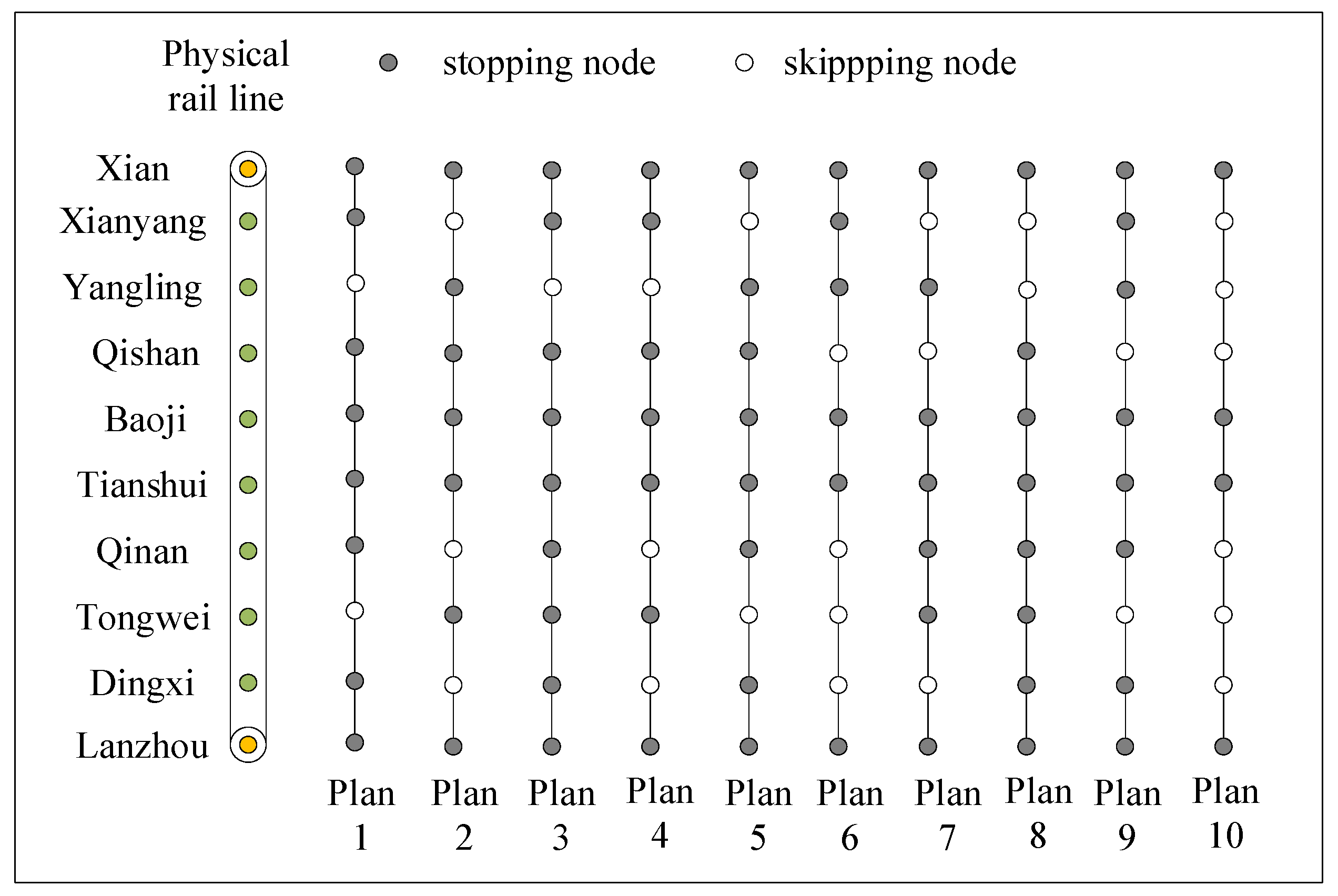
6.1. Experiment Scenario

In this section, we tested the models and algorithms on data from an actual high-speed rail corridor. Figure 9 shows the high-speed rail corridor from Lanzhou to Xi’an, with a total length of approximately 650 km. There are 10 nodes along the way that mark the site from the starting node at Lanzhou West Station to the terminal node at Xi’an North Station, in turn, as A–J. The distances between adjacent sites are shown in

Table 2. The distances between adjacent sites, $L_{i,i+1}$ (km).

A-B	B-C	C-D	D-E	E-F	F-G	G-H	H-I	I-J
105	85	64	51	139	44	51	68	44

.

Table 3. The passenger flow demand of each OD, $Q_{i,j}$ (person/day).

O/D	B	C	D	E	F	G	H	I	J
A	547	674	562	1096	1071	1124	889	1124	2020
B	-	300	562	449	300	612	112	350	562
C	-	-	675	512	675	137	337	175	450
D	-	-	-	750	675	437	637	312	150
E	-	-	-	-	749	675	412	187	2622
F	-	-	-	-	-	375	562	562	1498
G	-	-	-	-	-	-	687	687	375
H	-	-	-	-	-	-	-	887	749
I	-	-	-	-	-	-	-	-	687

shows the unidirectional traffic demand for 45 ODs from Lanzhou West Station to Xi’an North Station.

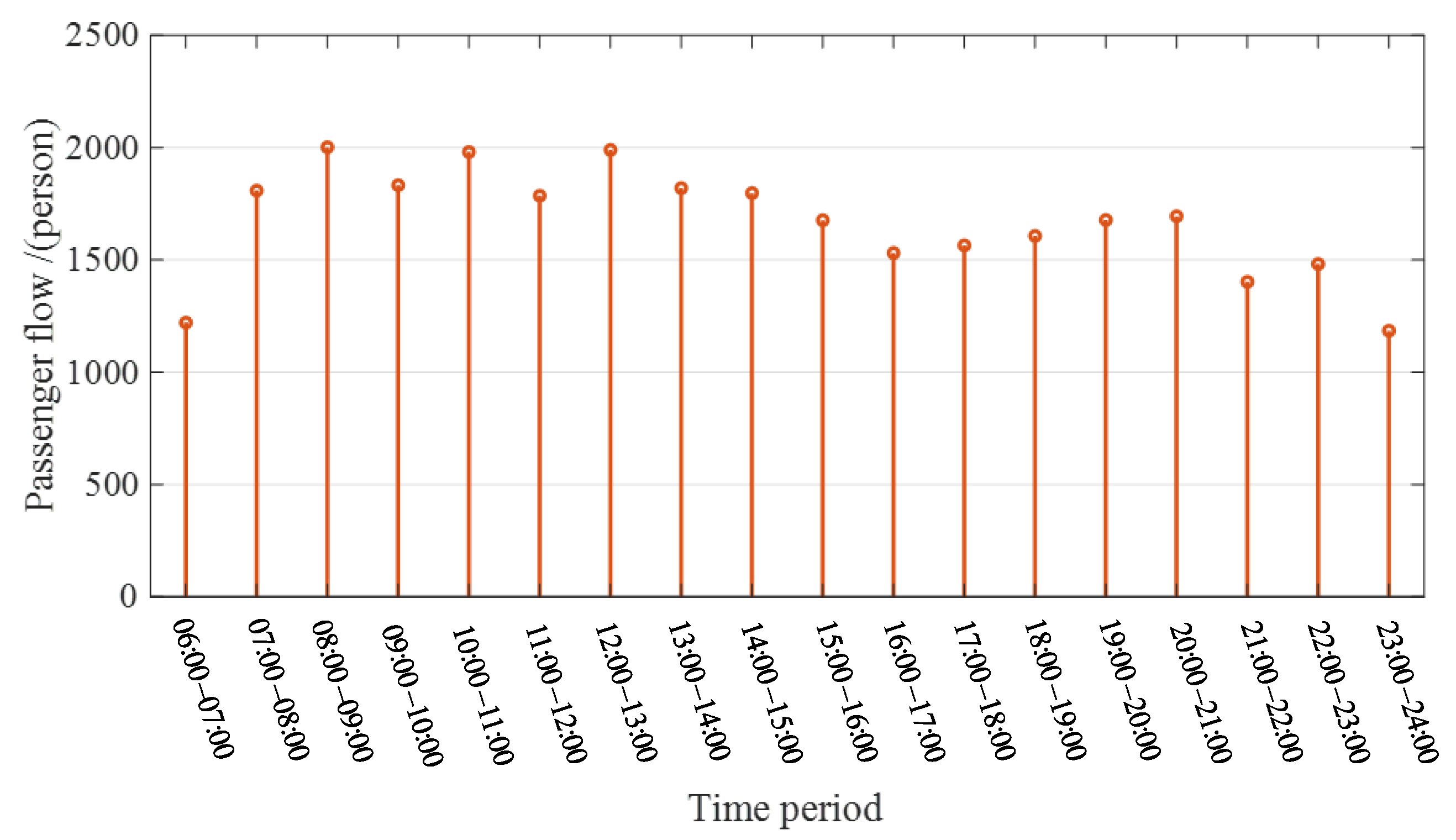
6.2. Setting the Parameters

The operation time of 06:00–24:00 of the Lan-xi high-speed rail corridor is divided into 18 time periods of one-hour intervals to obtain the time period set $H=${06:00–07:00… 23:00–24:00}. To obtain the convenience measure of each site in each time period, the author organized a questionnaire survey to investigate the expected departure time of the passengers along the nodes of the Lan-xi high-speed rail. According to the expected travel rate of the passengers in each time period at each node, the convenience, $g_i^h$, is determined. After the calculation, the convenience factor of each station in different time periods is shown in

Table 4. Convenience factor, ${\beta }_i$.

${\mathit{\beta }}_1$	${\mathit{\beta }}_2$	${\mathit{\beta }}_3$	${\mathit{\beta }}_4$	${\mathit{\beta }}_5$	${\mathit{\beta }}_6$	${\mathit{\beta }}_7$	${\mathit{\beta }}_8$	${\mathit{\beta }}_9$
0.228	0.2	0.266	0.24	0.2	0.226	0.25	0.23	0.28

. The other parameters in the model are shown in

Table 5. Other parameter values.

$\mathit{\alpha }$	$\mathit{k}$	$\mathit{m}$	$\mathit{U}$	${\mathit{\eta }}^{\mathit{h}\mathit{i}\mathit{g}\mathit{h}}$	$\mathit{\theta }$	$\mathit{\zeta }$
40	20	600	7200	0.356	1.2	0.328
${\eta }^{low}$	$\sigma$	${\sigma }^{\prime }$	${\sigma }^{″}$	$Ge$	${\vartheta }_{cor}$	${\vartheta }_{var}$
0.268	200	50	10	0.85	0.85	0.05

.

Referring to the existing train operation plan of the Lan-xi line, we use the ten stop plans shown in Figure 10 as an alternative set of stop plans.

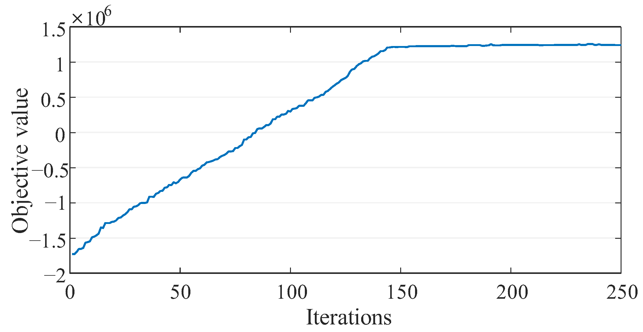
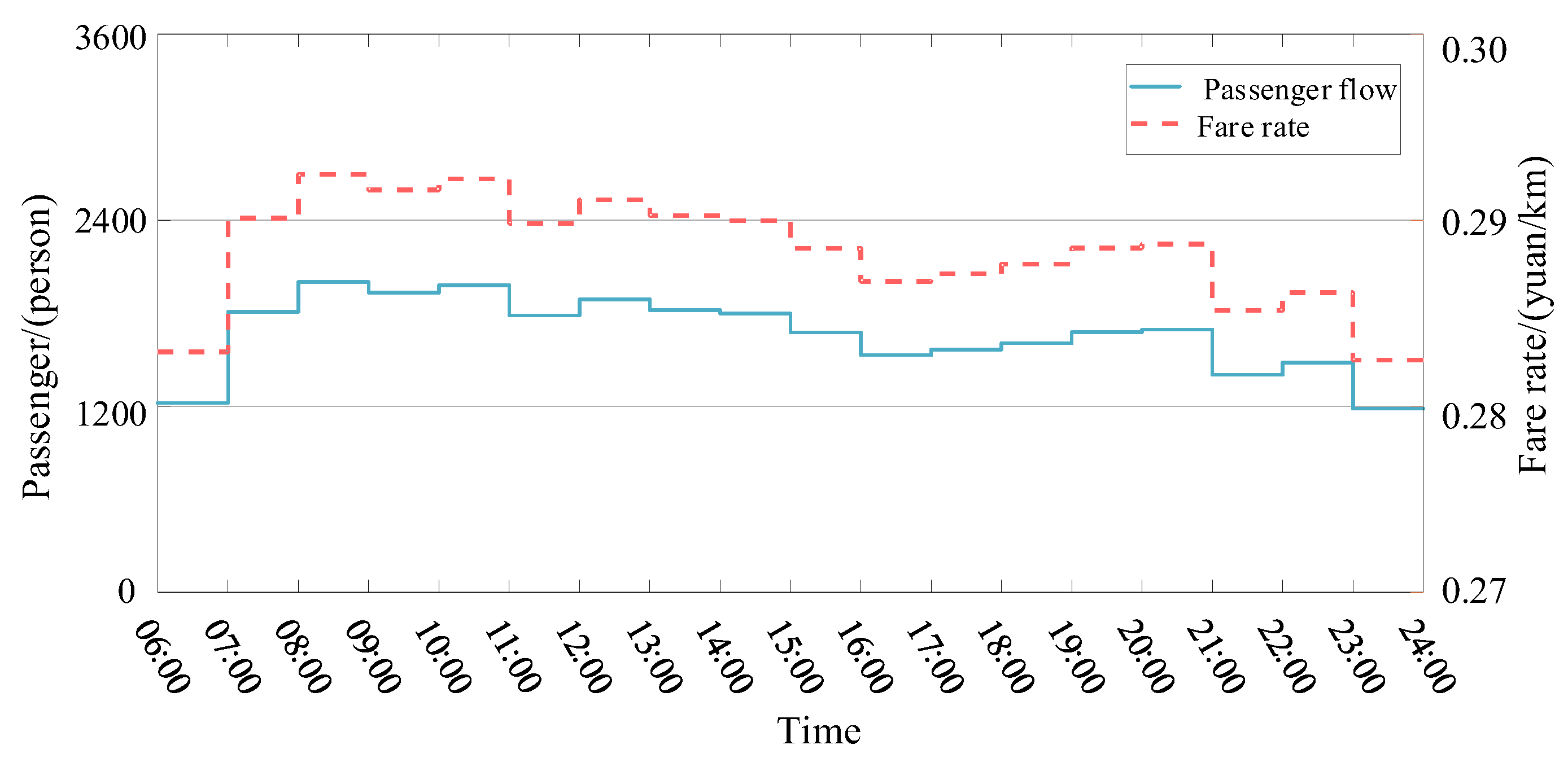
6.3. Analysis of the Results

Solving the model with MATLAB R2018a, Figure 11 shows the target value of each iteration calculated using the genetic algorithm for the first time. It can be seen from the figure that the target value increases as the number of iterations increases. It converges at approximately the 140th iteration and eventually converges to the vicinity of $1.2\times {10}^6$. The operation plan designed 65 trains a day for the rail enterprise. The number of trains of various types in each period is shown in Figure 12.

The satisfactory solution of the target values obtained by multiple genetic algorithms converges to approximately $1.2\times {10}^6$. In fact, the target value is always approximately $1.2\times {10}^6$ in multiple computations, but the operation plans are completely different. This shows that the operation plan to achieve a satisfactory solution for the rail benefit target value is not unique. When only pursuing the maximization of railway enterprise benefits, the railway enterprise has a variety of operation plan adjustment strategies.

Figure 13 shows the total number of passengers in each time period based on the operation plan obtained by the solution. It can be seen in the figure that under the flexible pricing strategy, the passenger flow distribution in each period is relatively balanced. Under the time period service capacity, there is no obvious peak period or valley period compared with the current passenger flow distribution in each time period in Figure 14.

When the operation plan is fixed, the passenger flow distribution in each time period is obtained by the fixed fare and dynamic pricing strategies. It can be clearly seen in Figure 15 that the passenger flow distribution at each time period is extremely unbalanced when the fare is fixed. The passenger flow is mainly concentrated in several periods in the morning, and there are fewer passengers in the afternoon and evening. In the absence of fare control, the passengers do not consider the impact of fares when choosing the departure time. Most passengers travel according to their desired time period. Comparing Figure 15 and Figure 16, the passenger flow distribution in each time period is more balanced under a dynamic pricing strategy. It shows that the dynamic pricing strategy has played a role in regulating the passenger flow during the period so that some passengers in the peak periods will choose to travel in other time periods to realize the peaking and filling of the time flow distribution, cutting the passenger flow during the peak periods and increasing the passenger flow during the low valleys. At the same time, this reduces the congestion and improves the travel experience of the passengers.

7. Conclusions

This paper focuses on the system optimization approach of high-speed railway corridor train operation planning based on a time flexible pricing strategy. Through solving the bi-level programming model and numerical experiments, the following conclusions are obtained:

(1)

This article has constructed a generalized travel cost function for passengers, which defines the convenience of passengers based on factors such as geographic location and regional economic level. It also takes into account the different experiences that passengers may have due to the level of crowding on the train and adjusts the ticket price accordingly. The article evaluates the convenience and comfort of passenger travel more comprehensively, providing ideas for the formulation of railway ticket pricing.

(2)

Passengers have different preferences for different travel periods. The transfer of railway passengers during each travel period results in changes in the travel cost of each path for the same OD. Based on Wardrop Equilibrium, this paper achieves a UE equilibrium state when the impedances are equal, at which time the total travel cost of passengers is minimal.

(3)

A flexible pricing strategy based on time slot passenger flow proposed in this paper increases the broad travel cost of passengers during peak periods by increasing fares and shifting the passenger flow from peak periods to low periods, relieving the pressure on railway operations during peak periods and improving the travel experience of passengers.

(4)

The bi-level programming model used in this paper ensures that railway revenue is maximized and total passenger travel costs are minimized and equal. While increasing the revenue of railway companies, it also satisfies passengers to spend less and improves passenger satisfaction.

In the next step in the future, we can consider introducing “pre-sale” tickets, seat classes and additional services for passengers during travel time in the model optimization and also consider a more detailed comparison of rail transport organization with air transport organization, including organization methods and route selection.

References

- Yang, W.; Chen, Q.; Yang, J. Factors Affecting Travel Mode Choice between High-Speed Railway and Road Passenger Transport—Evidence from China. Sustainability 2022, 14, 15745. [Google Scholar] [CrossRef]
- Li, H.; Li, X.; Xu, X.; Liu, J.; Ran, B. Modeling departure time choice of metro passengers with a smart corrected mixed logit model—A case study in Beijing. Transp. Policy 2018, 69, 106–121. [Google Scholar] [CrossRef]
- Wang, X.; Wang, H.; Zhang, X. Stochastic seat allocation models for passenger rail transportation under customer choice. Transp. Res. Part E Logist. Transp. Rev. 2016, 96, 95–112. [Google Scholar] [CrossRef]
- Wang, J.; Zhou, W.; Li, S.; Shan, D. Impact of personalised route recommendation in the cooperation vehicle-infrastructure systems on the network traffic flow evolution. J. Simul. 2018, 13, 239–253. [Google Scholar] [CrossRef]
- Zhang, P.; Ding, R.; Zhao, W.; Zhang, L.; Sun, H. Passenger Travel Path Selection Based on the Characteristic Value of Transport Services. Sustainability 2023, 15, 636. [Google Scholar] [CrossRef]
- Wang, Y.; Tang, T.; Ning, B.; van den Boom, T.J.J.; De Schutter, B. Passenger-demands-oriented train scheduling for an urban rail transit network. Transp. Res. Part C Emerg. Technol. 2015, 60, 1–23. [Google Scholar] [CrossRef]
- Kim, K.M.; Hong, S.-P.; Ko, S.-J.; Kim, D. Does crowding affect the path choice of metro passengers? Transp. Res. Part A Policy Pract. 2015, 77, 292–304. [Google Scholar] [CrossRef]
- Wang, J.; Niu, H. A distributed dynamic route guidance approach based on short-term forecasts in cooperative infrastructure-vehicle systems. Transp. Res. Part D Transp. Environ. 2019, 66, 23–34. [Google Scholar] [CrossRef]
- Mitropoulos, L.; Kortsari, A.; Mizaras, V.; Ayfantopoulou, G. Mobility as a Service (MaaS) Planning and Implementation: Challenges and Lessons Learned. Future Transp. 2023, 3, 498–518. [Google Scholar] [CrossRef]
- Khoshniyat, F.; Peterson, A. Improving train service reliability by applying an effective timetable robustness strategy. J. Intell. Transp. Syst. 2017, 21, 525–543. [Google Scholar] [CrossRef]
- Gabor, M.R.; Kardos, M.; Oltean, F.D. Yield Management—A Sustainable Tool for Airline E-Commerce: Dynamic Comparative Analysis of E-Ticket Prices for Romanian Full-Service Airline vs. Low-Cost Carriers. Sustainability 2022, 14, 15150. [Google Scholar] [CrossRef]
- Qin, J.; Qu, W.; Wu, X.; Zeng, Y. Differential Pricing Strategies of High Speed Railway Based on Prospect Theory: An Empirical Study from China. Sustainability 2019, 11, 3804. [Google Scholar] [CrossRef] [Green Version]
- Zhang, X.; Ma, L.; Zhang, J. Dynamic pricing for passenger groups of high-speed rail transportation. J. Rail Transp. Plan. Manag. 2017, 6, 346–356. [Google Scholar]
- Chou, J.-S.; Chien, Y.-L.; Nguyen, N.-M.; Truong, D.-N. Pricing policy of floating ticket fare for riding high speed rail based on time-space compression. Transp. Policy 2018, 69, 179–192. [Google Scholar] [CrossRef]
- Sato, K.; Sawaki, K. Dynamic pricing of high-speed rail with transport competition. J. Revenue Pricing Manag. 2011, 11, 548–559. [Google Scholar] [CrossRef]
- Tang, Z.; Qin, J.; Liu, H.; Du, X.; Sun, J. Optimal decisions of sharing rate and ticket price of different transportation modes in inter-city transportation corridor. J. Ind. Eng. Manag. 2015, 8, 1731–1745. [Google Scholar] [CrossRef] [Green Version]
- Zhang, X.; Luan, W.; Cai, Q.; Zhao, B. Research on Dynamic Pricing Between High Speed Rail and Air Transport under the Influence of Induced Passenger Flow. Inf. Technol. J. 2012, 11, 431–435. [Google Scholar]
- Zhang, X.; Li, L.; Le Vine, S.; Liu, X. An integrated pricing/planning strategy to optimize passenger rail service with uncertain demand. J. Intell. Fuzzy Syst. 2019, 36, 435–448. [Google Scholar] [CrossRef]
- Zheng, J.; Liu, J. The Research on Ticket Fare Optimization for China’s High-Speed Train. Math. Probl. Eng. 2016, 2016, 5073053. [Google Scholar] [CrossRef] [Green Version]
- Jin, F.L.; Tian, W.Q.; Wang, L. High-speed railway passenger flow equilibrium among trains of common lines based on travel behavior analysis under dynamic pricing. Transp. Lett. Int. J. Transp. Res. 2022, 1–16. [Google Scholar] [CrossRef]
- Yin, X.; Liu, D.; Rong, W.; Li, Z. Joint Optimization of Ticket Pricing and Allocation on High-Speed Railway Based on Dynamic Passenger Demand during Pre-Sale Period: A Case Study of Beijing–Shanghai HSR. Appl. Sci. 2022, 12, 10026. [Google Scholar] [CrossRef]
- Xu, X.; Xie, L.; Li, H.; Qin, L. Learning the route choice behavior of subway passengers from AFC data. Expert Syst. Appl. 2018, 95, 324–332. [Google Scholar] [CrossRef]
- Zhou, W.; Zou, Z.; Chai, N.; Xu, G. Optimization of Differential Pricing and Seat Allocation in High-Speed Railways for Multi-Class Demands: A Chinese Case Study. Mathematics 2023, 11, 1412. [Google Scholar] [CrossRef]
- Hamdouch, Y.; Ho, H.W.; Sumalee, A.; Wang, G. Schedule-based transit assignment model with vehicle capacity and seat availability. Transp. Res. Part B Methodol. 2011, 45, 1805–1830. [Google Scholar] [CrossRef]
- Li, W.; Zhu, W. A dynamic simulation model of passenger flow distribution on schedule-based rail transit networks with train delays. J. Traffic Transp. Eng. (Eng. Ed.) 2016, 3, 364–373. [Google Scholar] [CrossRef] [Green Version]
- Sun, S.; Szeto, W. Logit-based transit assignment: Approach-based formulation and paradox revisit. Transp. Res. Part B Methodol. 2018, 112, 191–215. [Google Scholar] [CrossRef]
- Fu, Q.; Liu, R.; Hess, S. A Review on Transit Assignment Modelling Approaches to Congested Networks: A New Perspective. Procedia-Soc. Behav. Sci. 2012, 54, 1145–1155. [Google Scholar] [CrossRef] [Green Version]
- Binder, S.; Maknoon, Y.; Bierlaire, M. Exogenous priority rules for the capacitated passenger assignment problem. Transp. Res. Part B Methodol. 2017, 105, 19–42. [Google Scholar] [CrossRef]
- Barrena, E.; Canca, D.; Coelho, L.C.; Laporte, G. Single-line rail rapid transit timetabling under dynamic passenger demand. Transp. Res. Part B Methodol. 2014, 70, 134–150. [Google Scholar] [CrossRef]
- Zhou, W.; Kang, J.; Qin, J.; Li, S.; Huang, Y. Robust Optimization of High-Speed Railway Train Plan Based on Multiple Demand Scenarios. Mathematics 2022, 10, 1278. [Google Scholar] [CrossRef]
- Niu, H.; Zhou, X.; Gao, R. Train scheduling for minimizing passenger waiting time with time-dependent demand and skip-stop patterns: Nonlinear integer programming models with linear constraints. Transp. Res. Part B Methodol. 2015, 76, 117–135. [Google Scholar] [CrossRef]
- Qi, J.; Yang, L.; Di, Z.; Li, S.; Yang, K.; Gao, Y. Integrated optimization for train operation zone and stop plan with passenger distributions. Transp. Res. Part E Logist. Transp. Rev. 2018, 109, 151–173. [Google Scholar] [CrossRef]
- Robenek, T.; Azadeh, S.S.; Maknoon, Y.; de Lapparent, M.; Bierlaire, M. Train timetable design under elastic passenger demand. Transp. Res. Part B Methodol. 2018, 111, 19–38. [Google Scholar] [CrossRef] [Green Version]
- Shang, P.; Li, R.; Yang, L. Optimization of Urban Single-line Metro Timetable for Total Passenger Travel Time under Dynamic Passenger Demand. Procedia Eng. 2016, 137, 151–160. [Google Scholar] [CrossRef] [Green Version]
- Zhang, T.; Li, D.; Qiao, Y. Comprehensive optimization of urban rail transit timetable by minimizing total travel times under time-dependent passenger demand and congested conditions. Appl. Math. Model. 2018, 58, 421–446. [Google Scholar] [CrossRef]
- Burdett, R.L.; Kozan, E. Scheduling Trains on Parallel Lines with Crossover Points. J. Intell. Transp. Syst. 2009, 13, 171–187. [Google Scholar] [CrossRef]
- Poon, M.H.; Wong, S.C.; Tong, C.O. A dynamic schedule-based model for congested transit networks. Transp. Res. Part B Methodol. 2004, 38, 343–368. [Google Scholar] [CrossRef]
- Nuzzolo, A.; Crisalli, U.; Rosati, L. A schedule-based assignment model with explicit capacity constraints for congested transit networks. Transp. Res. Part C Emerg. Technol. 2012, 20, 16–33. [Google Scholar] [CrossRef]
- Di, Z.; Yang, L.; Qi, J.; Gao, Z. Transportation network design for maximizing flow-based accessibility. Transp. Res. Part B Methodol. 2018, 110, 209–238. [Google Scholar] [CrossRef]
- Farvaresh, H.; Sepehri, M.M. A single-level mixed integer linear formulation for a bi-level discrete network design problem. Transp. Res. Part E Logist. Transp. Rev. 2011, 47, 623–640. [Google Scholar] [CrossRef]