Article

Pavement Roughness Prediction Using Explainable and Supervised Machine Learning Technique for Long-Term Performance

1
Department of Civil Engineering, Faculty of Engineering, Sri Lanka Institute of Information Technology, Malabe 10115, Sri Lanka
2
Institute for Sustainable Industries & Liveable Cities, Victoria University, P.O. Box 14428, Melbourne, VIC 8001, Australia
3
College of Sport, Health and Engineering, Victoria University, P.O. Box 14428, Melbourne, VIC 8001, Australia
4
Department of Civil Engineering and Construction, Faculty of Engineering and Design, Atlantic Technological University, F91 YW50 Sligo, Ireland
*
Authors to whom correspondence should be addressed.
Sustainability 2023, 15(12), 9617; https://doi.org/10.3390/su15129617
Submission received: 18 May 2023 / Revised: 9 June 2023 / Accepted: 13 June 2023 / Published: 15 June 2023

Abstract

:
Maintaining and rehabilitating pavement in a timely manner is essential for preserving or improving its condition, with roughness being a critical factor. Accurate prediction of road roughness is a vital component of sustainable transportation because it helps transportation planners to develop cost-effective and sustainable pavement maintenance and rehabilitation strategies. Traditional statistical methods can be less effective for this purpose due to their inherent assumptions, rendering them inaccurate. Therefore, this study employed explainable and supervised machine learning algorithms to predict the International Roughness Index (IRI) of asphalt concrete pavement in Sri Lankan arterial roads from 2013 to 2018. Two predictor variables, pavement age and cumulative traffic volume, were used in this study. Five machine learning models, namely Random Forest (RF), Decision Tree (DT), XGBoost (XGB), Support Vector Machine (SVM), and K-Nearest Neighbor (KNN), were utilized and compared with the statistical model. The study findings revealed that the machine learning algorithms’ predictions were superior to those of the regression model, with a coefficient of determination (R2) of more than 0.75, except for SVM. Moreover, RF provided the best prediction among the five machine learning algorithms due to its extrapolation and global optimization capabilities. Further, SHapley Additive exPlanations (SHAP) analysis showed that both explanatory variables had positive impacts on IRI progression, with pavement age having the most significant effect. Providing accurate explanations for the decision-making processes in black box models using SHAP analysis increases the trust of road users and domain experts in the predictions generated by machine learning models. Furthermore, this study demonstrates that the use of explainable AI-based methods was more effective than traditional regression analysis in IRI prediction. Overall, using this approach, road authorities can plan for timely maintenance to avoid costly and extensive rehabilitation. Therefore, sustainable transportation can be promoted by extending pavement life and reducing frequent reconstruction.

1. Introduction

Pavement condition has a direct impact on user comfort as well as pavement performance. Roughness is an indicator that reflects pavement surface conditions and indirectly reflects pavement structural conditions [1,2]. There are various methods to quantify roughness, and among those, the most common parameter is the International Roughness Index (IRI), defined as ASTM E1364-95 [3]. The IRI is calculated based on the quarter-car model, which reflects the vertical acceleration responses due to irregularities on the pavement [4]. Traffic load, pavement aging, environmental factors, and construction defects are known to be the main reasons for pavement deterioration [2,5,6,7].
Generally, IRI prediction has relied on statistical methods such as linear and nonlinear regression. However, these models have some limitations. This is because the relationships between the IRI and predictor variables are mostly nonlinear [8,9], and conventional regression analysis cannot accurately predict these relationships [10,11]. Moreover, additional assumptions have to be considered in statistical approaches for data preparation [9]. Additionally, regression models tend to yield less accurate results when the dataset is larger and the number of predictor variables is higher [9,12,13]. As a result, machine learning algorithms have been introduced more recently, and they have been shown to outperform regression models in most cases [14,15]. However, machine learning models can be ineffective in some situations due to the lack of explainability of the generated outputs [16].
To address the limitations associated with regression analysis as well as machine learning models, this study suggests a novel approach that employs a supervised and explainable machine learning technique to predict the IRI. The approach involves the use of five different machine learning models to predict the IRI using two predictor variables, pavement age and cumulative traffic volume, which are commonly used in predicting the IRI for long-term performance evaluation. The dataset used in this study comprised 259 road segments of asphalt concrete pavement with IRI values on Sri Lankan arterial roads. Model fitting was assessed using the coefficient of determination (R2) and the mean absolute error (MAE). Moreover, to address the lack of explainability in machine learning models, SHapley Additive exPlanations (SHAP) analysis was used to interpret factor importance in IRI prediction. Providing accurate explanations for decision-makers using SHAP analysis would reduce the black box nature of machine learning models, which will increase the trust of both road users and domain experts in the results generated by machine learning.
This study aimed to evaluate the effectiveness of traditional regression models as well as machine learning models with post hoc explanations in predicting IRI progression. This study is unique for several reasons: (a) it is the first study in the Sri Lankan context to use supervised machine learning with pavement age and traffic data to predict the IRI; (b) it employs different machine learning algorithms to assess their suitability in predicting the IRI and compares their performance with that of traditional regression; (c) it uses post hoc methods or explainable artificial intelligence (AI) to interpret the machine learning models. Overall, using accurate advanced technologies and the sustainable practices proposed in this study can effectively contribute to sustainable transportation. Further, they will help to improve road safety, reduce tire wearing and tearing, and decrease fuel consumption and emissions, thereby promoting a sustainable transportation system.

2. Background Study

2.1. IRI Prediction Models

In general, pavement condition is primarily assessed by considering pavement distress and surface roughness. There are various indices available to measure pavement roughness, such as Ride Number (RN), IRI, Half-car Roughness Index (HRI), Mays Ride Meter (MRM), Quarter-car Index (QI), and Present Serviceability Index (PSI) [17]. Among these, the IRI is a widely accepted parameter for measuring pavement roughness, and it is reported in m/km or inch/mi. The IRI assesses the road surface roughness based on how a vehicle responds to the actual roughness profile [17]. An algorithm is used to calculate the IRI, which simulates how a specific vehicle may react to road roughness, as shown in Equation (1) [18].
IRI = 0 T | z ˙ u z ˙ s | L dt
where, z ˙ u is the vertical velocity of the axle, z ˙ s is the vertical velocity of the vehicle body, L is the length of the measured distance, and T is the time duration for the roughness measurement.
The IRI is one of the most reliable parameters to measure road usability [19,20]. IRI progression in the long-term is influenced by cumulative traffic load, pavement age, and the quality of paving materials [21]. Among those, traffic load and pavement age are considered two critical factors in IRI prediction models since an increase in heavy truck volume causes higher pavement damage [22]. Further, environmental factors play a significant role in long-term performance evaluation, with climate factors such as precipitation, temperature, air humidity, and moisture deficit affecting IRI progression [9]. Therefore, pavement age, which reflects long-term performance, is an important factor in predicting the IRI. To estimate the IRI, regression models have used empirical, mechanistic-empirical, or probabilistic models [23]. Table 1 provides a summary of IRI prediction models developed by incorporating several predictor variables such as pavement age, traffic factors, environmental factors, distress, etc.

2.2. Use of Machine Learning Approach for Predicting IRI

Machine learning models are automated models used in data analysis that are capable of detecting patterns in data and using them to predict future data or make decisions under uncertainty [30]. There are two types of machine learning techniques, supervised and unsupervised learning, which differ in their goals. The objective of supervised learning is to predict the outcome measure based on several inputs, while in unsupervised learning, the focus is on describing relationships and patterns among a set of input measures. Supervised learning can be used in both classification and regression problems. Recently, researchers have been interested in predicting pavement conditions using machine learning models [10,14,30]. However, some have also employed metaheuristic algorithms, such as particle swarm optimization and gene expression programming, fuzzy algorithms [31], hybrid models, and combined methods with machine learning techniques [11,32].
Most machine learning models employed to predict the IRI rely on supervised learning for the purpose of regression analysis. To achieve this, supervised learning models utilize labeled data to predict IRI values where the values already exist. The dataset is partitioned into two subsets: training and testing sets. Supervised models are developed using the training set, and the accuracy of the model is assessed using the testing set. On the other hand, regression models involve an equation with multiple predictors, including the IRI as a response variable. The parameter values are estimated using the available data, and the model is subsequently utilized to make predictions. This approach differs from supervised machine learning models, which aim to find a function that operates to predict the response [33].
Random Forest (RF) and Support Vector Machine (SVM) are the two most used machine learning techniques for predicting the IRI, according to the literature. Tree-based techniques, gradient boosting, and K-Nearest Neighbor (KNN) have also been used by researchers for IRI prediction worldwide. Most researchers have relied on the long-term pavement performance (LTPP) dataset as the primary data source for investigating IRI prediction. However, researchers from various countries have employed their own collected data to explore IRI prediction using machine learning techniques. Recent studies focused on predicting the IRI using machine learning models are presented in Table 2.
The majority of the previous studies on pavement performance prediction using machine learning or deep learning did not evaluate their models using feature importance evaluation methods or post hoc explanation methods. As a result, end-users have limited knowledge about the importance and interaction of features, the dependencies of features, and how the machine learning model works. This lack of transparency in machine learning models is a critical issue, especially in high-stakes contexts such as pavement performance prediction where errors can lead to significant consequences. Thus, providing explanations for the results generated by machine learning models is essential due to the absence of pre-defined relationships between variables in these models.

3. Materials and Methods

3.1. Study Area

The study area selected was 259 km of arterial road segments in Sri Lanka, all of which were asphalt concrete roads with different traffic conditions for which the average annual daily traffic varied from 9000 to 115,000 veh/day. The IRI values and traffic data for this study were obtained from the Planning Division, Road Development Authority, Sri Lanka. Moreover, pavement maintenance history data were obtained from the same authority and road construction company databases [42,43].
The study took into consideration two variables, pavement age and cumulative traffic volume, to forecast the IRI. During the data analysis phase, pavement age was referred to as AGE, while cumulative traffic was referred to as CUMTRAF. Table 3 provides the summary of descriptive statistics of the variables. The independent variables were extracted for all roadways with asphalt pavement from 2013 to 2018 with IRI values in the database. The IRI value was taken as the mean roughness index, which was calculated as the average of the inner and outer lane IRI values. Climate variables were not considered in the IRI prediction as there was limited climate variation in the study area, which was in line with previous studies [28,41,44,45,46]. The histograms of the model’s variables, depicted in Figure 1, demonstrate that their distributions differed and that most of them were nonlinear.

3.2. Data Processing

Python version 3.7 was used for data analysis, and the machine learning models were implemented using the scikit-learn library, a Python-based machine learning toolkit [47]. A total of 259 data points, in which each section was 1 km long, were included in the analysis. To train and test the models, the dataset was divided 70% for training and 30% for testing. A correlation analysis was conducted and the correlation coefficient between pavement age and cumulative traffic volume was found to be 0.57, indicating a moderate correlation between the two variables. A higher correlation between predictors can lead to inaccurate parameter estimation and large standard error [2,48]. This discussion on IRI prediction using regression analysis can be inaccurate if the predictor variables are dependent on each other, leading to violation of the regression analysis. Thus, to eliminate this issue and to explore the relationships between pavement age and cumulative traffic with the IRI, we used five machine learning models.

3.3. Machine Learning Models

3.3.1. Extreme Gradient Boosting

Extreme Gradient Boosting (XGB) is a highly effective method for data classification [49]. It is one of the highly scalable, end-to-end tree-boosting systems used in machine learning [50]. The workflow of XGB can be explained as follows.
Consider a Classification And Regression Tree (CART) model with a set of K E i |   i   1 K nodes. For each tree, k th total prediction scores at leaf node f k are predicted to obtain the final prediction output of class label y ^ i , as expressed in Equation (2).
y ^ i =   φ ( x i ) = k = 1 k f k ( x i ) ,   f k   F
Equation (3) gives a regularization step that improves the validity of the results. Where the K score for all charts is represented by set F and x i denotes the training set.
( φ ) = i l ( y ^ i ,   y i ) + k Ω ( f k ) ,
where l represents the differentiable loss function, defined by computing the error difference between the target y i and the predicted class label y ^ i . The second part performs a penalization, Ω, on model complexity to avoid the overfitting problem. The penalty function Ω is calculated by Equation (4).
Ω ( f ) =   γ T + 1 2 λ j = 1 T w j 2
Here, w stores the value of weights for each leaf, whereas T represents the leaves in the tree. γ and λ are known as configurable parameters that control the level of regularization.

3.3.2. Decision Tree

Decision Tree analysis is an established analytical method in data mining, which generates a tree-based model to predict the values of a dependent variable based on independent variables. Compared to traditional regression modeling, Decision Tree analysis excels at identifying determinants. One of its strengths is that it does not require specific data format rules and can analyze continuous independent variables, categorical variables, and multivariate, unordered categorical variables [51]. Decision Tree analysis is a non-parametric statistical technique that does not make assumptions about the functional form or distribution of data [52]. It can also explore interaction effects between independent variables and address multicollinearity issues [53].
The decision tree-building process involves two stages: tree building and tree pruning. The tree-building process involves classifying the preliminary record level by level until it is no longer possible or necessary to split based on certain criteria to generate the tree. Tree models can be classified into two categories based on the dependent variable: classification and regression trees. Commonly used algorithms include CHAID (Chi-square Automatic Interaction Detector), CRT (Classification and Regression Tree), and QUEST (Quick, Unbiased, Efficient, and Statistical Tree). The CRT algorithm segments the data and constructs a tree model that maximizes the homogeneity of the values of the dependent variable within the nodes [53].

3.3.3. K-Nearest Neighbor

Introduced in 1951, the KNN rule is a distribution-free, statistical pattern classification method that has gained popularity since the 1960s due to the advancement of computational power [38]. The KNN algorithm compares a given testing tuple to a set of similar training tuples and learns by determining the class based on the K number of nearest neighbors [48]. Although statisticians have adopted KNN as a machine learning approach for 50 years, it is still widely used in pattern recognition and classification due to its unique features.
KNN is considered a “lazy learner” or “instance-based learner” because it stores the given training tuple and waits until it receives a testing tuple to perform a generalization based on similarity or distance, unlike other models that use the prediction model to predict the testing tuples they receive. Generally, KNN uses either Euclidean distance or cosine similarity methods to compare the training and testing tuples while this study used the Euclidean distance [54]. Considering two tuples for example, X 1 = ( x 11 ,   x 12 ,   , x 1 n )   and   X 2 = ( x 21 , x 22 , , x 2 n ) , the Euclidean distance of two tuples can be obtained from Equation (5).
d i s t   ( x 1 ,   x 2 ) = i = 1 n ( x 1 i x 2 i ) 2

3.3.4. Random Forest

RF is an ensemble learning method that uses decision trees and is known to be a meta-estimator-based algorithm. RF fits multiple decision trees for different subsamples for a given dataset and averages the results to increase the accuracy of predictions by avoiding overfitting [55]. Moreover, RF can be used for both classification and regression modeling because of the higher performance level compared to decision trees. RF is easy to conceptualize and implement since it can handle a large number of input variables [55]. However, one of its main limitations is that the internal decision logic can be difficult to understand when many decision trees are involved. Additionally, the ensemble approach is computationally expensive, which can reduce the algorithm’s efficiency when time is a constraint. RF is versatile and has been utilized in various domains.

3.3.5. Support Vector Machine

SVM is a popular algorithm used for predicting the IRI. Even with a small number of training data points, SVM can approximate a nonlinear relationship [8]. SVM is applied to both classification and regression problems, and it was first introduced by Boser et al. in 1992 [8]. In Support Vector Regression (SVR), which is used in SVM’s regression analysis, the objective is to fit the model to the dataset by defining an acceptable error in the model, known as the margin, and minimizing that margin. If some points in the dataset fall outside the margin, the algorithm assigns a penalty to these points, controlled by parameter C in the model. Regularization is the process of adding a penalty term to the cost function. C is the complexity parameter that controls the trade-off between having a big margin versus correctly classifying all the training data. If C has a small value, there will be a larger margin with more error in the training dataset, but a more robust fit. Conversely, if C has a large value, there will be a smaller margin with less error in the training dataset, but a less robust model. While linear regression aims to minimize the sum of squares error, SVR aims to minimize the coefficients. The error term is controlled by constraints, and a slack variable is considered for the data points outside the epsilon. The SVR objective function is given in Equation (6) and the SVR constraints are shown in Equation (7).
min 1 2 | w | 2 + C i = 1 n | i |
| y i w i x i |   + | i | ,   i   0  
Here, w stores the value of weights for each leaf whereas T represents the leaves in the tree. γ and λ are known as configurable parameters that control the level of regularization. To effectively use SVR, it is important to normalize the features and impute missing values. In contrast, ensemble models do not require filling in missing values. Nonetheless, by utilizing the Lagrangian method, SVR can efficiently solve this quadratic optimization problem.

3.4. Explainable Artificial Intelligence

Explainable AI aims to enhance the confidence of domain experts and machine learning users by providing an understanding of the causality behind machine learning [56,57]. Intrinsic explanations are typically sufficient for simple models such as decision trees, but extrinsic (post hoc) interpretations are needed for more complex models (e.g., LIME [58], RISE [59], SHAP [60], etc.). These explanations are essential to provide transparency and visibility to ML predictions by revealing hidden reasoning.

SHAP (SHapley Additive exPlanations)

SHAP analysis was introduced by Lundberg and Lee in 2017 and it can provide explanations for a model as a whole or for each individual instance [60]. The fundamental principle behind SHAP is based on game theory, which associates the contribution of a player to the game. One of the main applications of SHAP is to obtain a single and consistent measure of feature importance. We used Tree-SHAP for the present study, using Equation (8) to compute the Shapley value.
f ( y ) = ϕ o + i = 1 N ϕ i y i
where f is the explanation model, N is the maximum size of coalition, and ϕ denotes the feature attribution. Equations (9) and (10) are used to calculate the feature attribution.
ϕ i = S   { 1 , , p } \ { i } | S | ! ( p | S | 1 ) ! p ! [ g x ( S { i } ) g x ( S ) ]
where ;   g x ( S ) = E [ g ( x ) | x S ]
The term S denotes a subset of input features and x is a vector of feature values of instance (the instance needs to be interpreted). The Shapley value is obtained through the value function ( g x ), p is the number of features, and E [ g ( x ) | x K ] expresses the expected value of the function on subset S.

4. Results

4.1. Multiple Regression Analysis

The estimation of the IRI involved utilizing pavement age and cumulative traffic volume as variables. Firstly, the correlations between both independent variables and the IRI were assessed using Pearson coefficients (Table 4). AGE showed a high correlation of 0.83 while CUMTRAF showed a low correlation of 0.58. Secondly, the relationship between the IRI and each predicting variable was evaluated to determine the model that best fit the data (Table 5). Different types of models were used to fit the data, including cubic, quadratic, linear, exponential, logarithmic, and logistic, with different evolution trends. From the results, it was observed that both AGE and CUMTRAF had the best correlations in the cubic model, followed by the quadratic and linear models. Even though the cubic model had the highest R2 value, the model shape was not matched with IRI progression in general. Thus, the quadratic equation was selected as the best representative model. For the multiple regression analysis, both variables were converted into quadratic transformation components as AGE2 and CUMTRAF2.
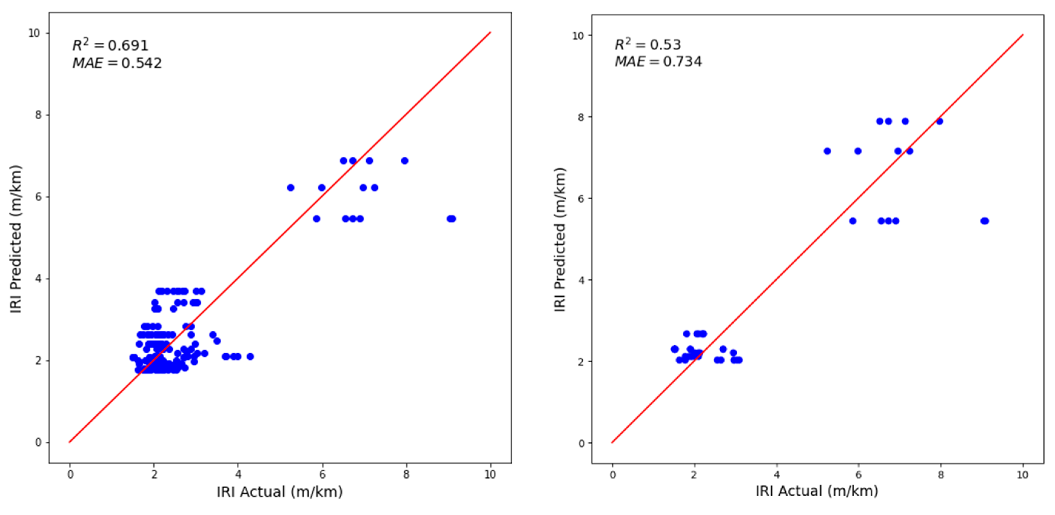
Firstly, the multiple linear regression model without transformed variables (AGE and CUMTRAF only) achieved an R2 value of 0.69 for the training dataset. To verify the training model, a testing dataset (30% of the data) was utilized and a corresponding R2 value of 0.53 and MAE value of 0.73 were obtained, as depicted in Figure 2. The training regression model as a function of pavement age and cumulative traffic for the training dataset is shown in Equation (11).
IRI t = 1.569 + 0.305 × AGE + 0.010 × CUMTRAF   [ R 2 = 0.69 ]
where IRIt is the IRI of road segment after ‘t’ number of years, AGE is the pavement age after the latest rehabilitation/reconstruction in years, and CUMTRAF is the cumulative traffic volume in number of vehicles in millions after ‘t’ number of years.
Moreover, the coefficients of the regression model variables are presented in Table 6. All the coefficients had p-values less than 0.05, indicating that the dependent variables’ effects were statistically significant.
IRI t = 1.668 + 0.336 × AGE    [ R 2 = 0.67 ]
As in Figure 2 and Table 6, it was observed that both pavement age and cumulative traffic had positive relationships with the IRI, which indicated that when the traffic and age increased, the IRI tended to increase. Moreover, the initial IRI value varied between 1.410 and 1.733 m/km at a 95% confidence interval, which agreed with most of the initial IRI values in the Asian context. Further, a sensitivity analysis was conducted using backward elimination criteria. It revealed that removing the cumulative traffic variable would only reduce the model accuracy by 2%, as in Equation (12). The sensitivity analysis showed that the IRI value increased by about 0.336 m/km per year, since the impact of cumulative traffic was much less than that of pavement age. Furthermore, Figure 2 shows that lower IRI values of less than 5 m/km were accurately predicted by the multiple regression model. However, when the IRI value was more than 5 m/km, the predictability was much less than at lower IRI values.
Secondly, additional multiple regression models were tested by combining different variables alongside their quadratic transformations (AGE2, CUMTRAF2). Apart from the R2 values, the significance of the variables in the analyzed models is presented in Table 7. From the results in Table 7 it can be observed that introduction of quadratic transformations (AGE2, CUMTRAF2) significantly enhanced the model accuracy compared to the linear models. Moreover, the last model in Table 7 was found to have the best fit. However, the significance of AGE in that model was low, which implied that the second model with AGE, CUMTRAF, and CUMTRAF2 as components was the best representative model. Comparing the linear regression model described by Equation (11) and the second model showed that the R2 value drastically increased due to the inclusion of quadratic transformed CUMTRAF2. Overall, it could be observed that pavement age and cumulative traffic volume significantly contributed to IRI progression, while better predictions could be obtained with the inclusion of quadratic-transformed variables. However, to further improve IRI predictability, the study focused on using machine learning models with explainable AI to explain the feature importance.

4.2. Machine Learning Models

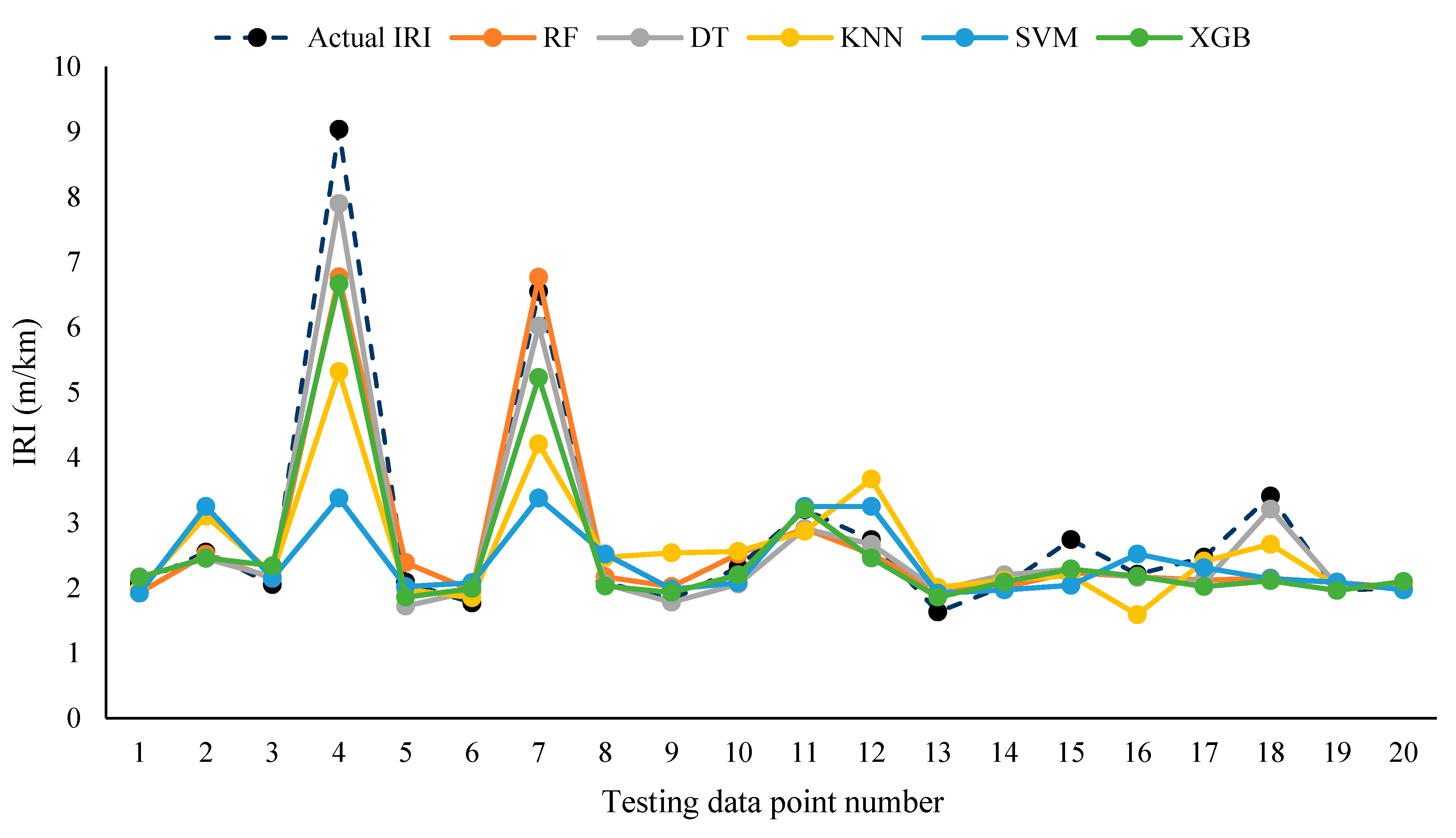
The research used 181 instances for training and 78 for testing, using AGE and CUMTRAF as independent variables. Figure 3 illustrates how well the five models predicted the actual IRI values, with 20 random testing points selected from the 78 testing data points. The predicted IRI values from all five machine learning models were compared with the actual IRI values. The models with closer predicted values to the actual IRI values were considered to have better predictions. For instance, the SVM model had a less accurate prediction for testing data point 4, with the maximum distance to the actual point. As an example, all five machine learning models accurately predicted testing data points 19 and 20. However, it should be noted that Figure 3 only represents 25% of the testing set, while individual behaviors varied based on their predictability.
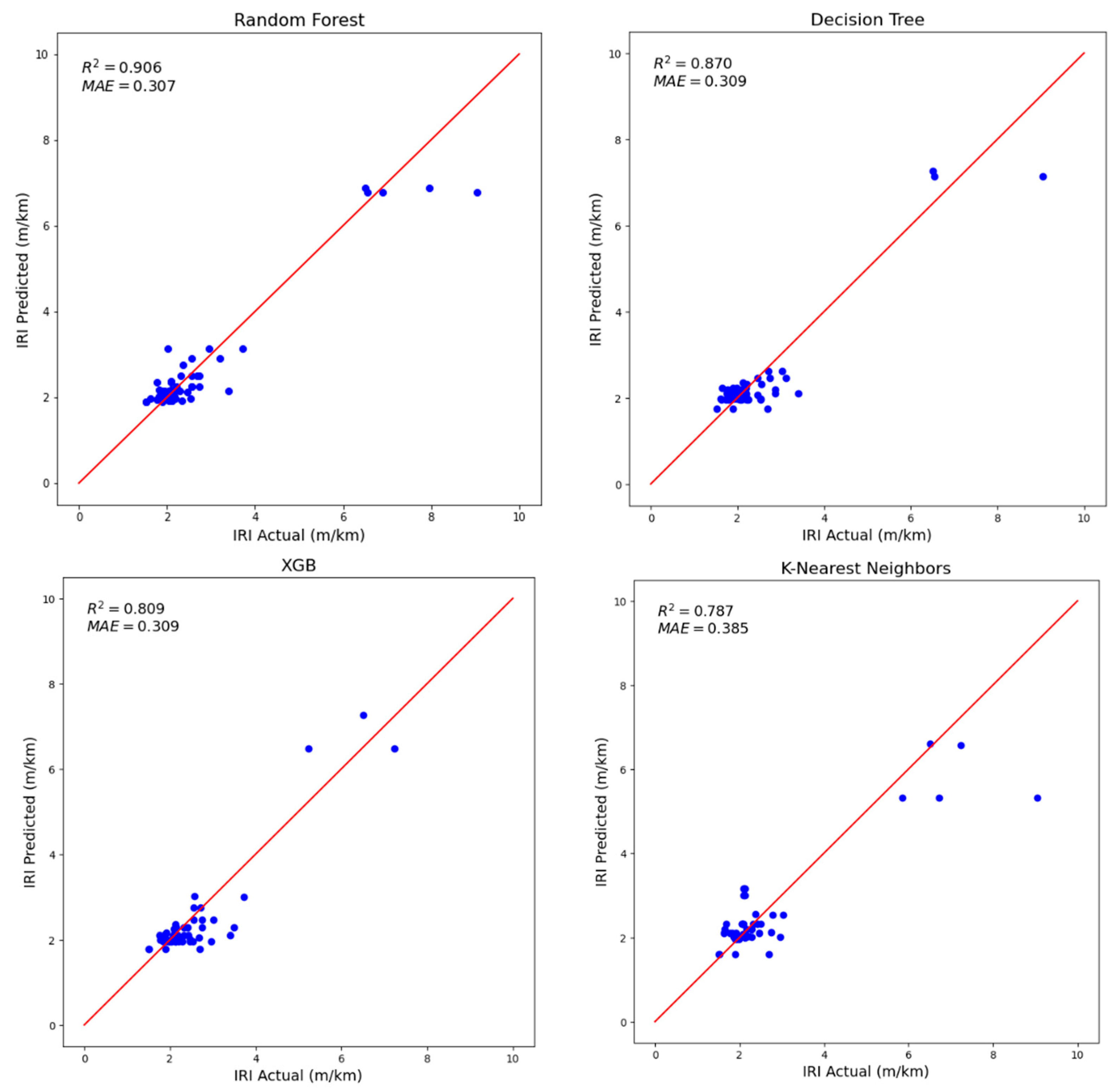
Table 8 presents the predictability statistics of the IRI for each machine learning regressor. Among the models, the RF model was found to be the best model with an R2 value of 0.906 and MAE value of 0.310 for the testing dataset. The R2 value explains the proportion of variance in the IRI that is accounted by AGE and CUMTRAF. Moreover, the MAE value represents the average absolute difference between the actual and observed IRI, regardless of the direction of error. Additionally, the DT, XGB, and KNN models performed better than the LR model, with R2 values greater than 0.75. However, the SVM model showed poor predictability compared to all the other machine learning models as well as the LR model. Therefore, it could be concluded that all of the machine learning models, except for SVM, exhibited versatility and efficiency in predicting the IRI from AGE and CUMTRAF and performed better than traditional regression methods. Further, Figure 4 shows the model validation results on the testing dataset for all five machine learning models.

4.3. Machine Learning Global Explanation

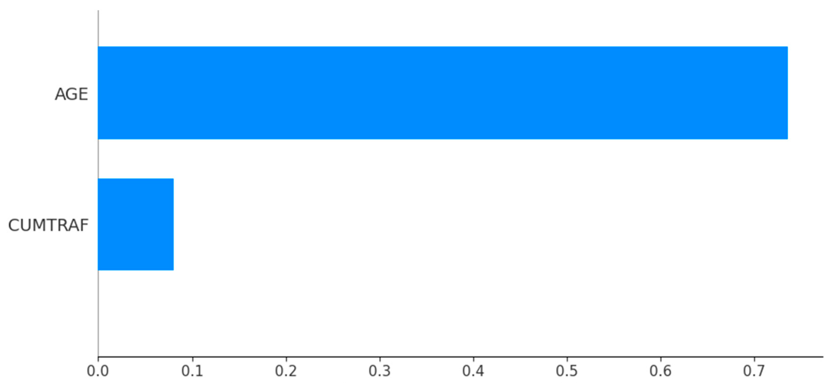
Further, SHAP analysis was used to analyze the output of the RF model and predict the global behavior of the IRI with respect to AGE and CUMTRAF. The global explanation obtained from SHAP analysis is presented in Figure 5, where blue and red colors are used to represent low and high values of each feature, respectively. The features are ranked according to their importance, and AGE was found to have the most significant impact on the IRI. From Figure 5 it was observed that when pavement age increased, the IRI value drastically increased. However, both low and high values for CUMTRAF were clustered around zero, which indicated that the importance of CUMTRAF was not significant in the model output. This provided sufficient evidence that cumulative traffic had a low impact on IRI progression compared to pavement age. Moreover, this feature behavior followed the same trend as in the multiple regression model. Figure 6 explains the feature importance using a horizontal bar chart. The plot consists of a horizontal bar, where each bar represents a feature in the dataset. The bar length indicates the magnitude of the Shapley value for that feature. As in Figure 6, AGE and CUMTRAF had mean Shapley values of 0.7, and 0.1, respectively. This result indicated that pavement age was highly important, about seven times more important than cumulative traffic, in IRI prediction for the given data. However, there can be some inaccuracy in SHAP analysis results due to its assumption of additivity when analyzing complex nonlinear relationships [61]. Since the data used in this study did not have a complex nonlinear relationship, the SHAP analysis results were acceptable.
Overall, these results highlighted the importance of incorporating multiple contributing factors to IRI progression and the potential of explainable AI to improve model explanations. According to the results, the explainable AI approach provided a deeper understanding of IRI progression and revealed hidden sensitive behavior based on machine learning predictions.

5. Summary and Conclusions

It is important to consider the impact of pavement age and cumulative traffic on long-term IRI prediction modeling while most of the previous studies used statistical models to predict pavement performance. Even though machine learning models can be used in such predictions due to the complexity of the analysis, the black box nature of these models has limited their use. To address both issues, the researchers in this study showed the applicability of explainable AI in IRI prediction compared with regression-based modeling using 259 arterial road segments in the Sri Lankan national road network.
The study used five machine learning techniques, RF, DT, XGB, KNN, SVM, and the traditional LR model, to predict the IRI while using cumulative traffic and pavement age as predictor variables. The researchers evaluated the models using performance metrics R2 and MAE, with the LR model achieving R2 and MAE values of 0.530 and 0.732, respectively, for the testing dataset. Moreover, various nonlinear models were used to improve the predictability of the regression models using quadratic transformations of AGE and CUMTRAF. It was found that the R2 value increased to 0.830 in the regression model including AGE2 and CUMTRAF2 as predictor variables. The results showed that the machine learning methods were more effective than the LR model in predicting the IRI, with the RF model having the highest prediction performance with an R2 value of 0.906, followed by DT with an R2 value of 0.870 and XGB with an R2 value of 0.809. The global explanation of the data models was performed using SHAP analysis, which revealed that pavement age was the most dominant predictor for Sri Lankan arterial roads.
In conclusion, explainable AI is a preferable approach for domain experts such as highway engineers when working with large amounts of roadway data. Moreover, the high-stakes and sensitive factors affecting IRI progression require accurate prediction models, and explainable AI offers a better platform with accurate and robust techniques compared to traditional statistical approaches that have limitations in their analysis features. Finally, accurate IRI prediction is essential for sustainable transportation as it helps to extend the service life of pavement by minimizing the frequency of extensive maintenance while minimizing the overall environmental impact of road infrastructure.

Author Contributions

Conceptualization, K.S., S.S. and U.R.; methodology, K.S.; software, S.S.; validation, K.S., U.R. and N.M.; formal analysis, K.S. and S.S.; investigation, K.S. and S.S.; resources, K.S. and S.S.; data curation, K.S.; writing—original draft preparation, K.S. and S.S.; writing—review and editing, K.S., U.R. and N.M.; visualization, S.S.; supervision, U.R. and N.M.; project administration, U.R.; funding acquisition, U.R. and N.M. All authors have read and agreed to the published version of the manuscript.

Funding

This research received no external funding.

Institutional Review Board Statement

Not applicable.

Informed Consent Statement

Not applicable.

Data Availability Statement

Data is available on request from the corresponding author.

Conflicts of Interest

The authors declare no conflict of interest.

References

  1. Golova, E.; Evtyukova, S.; Protsuto, M.; Evtyukov, S.; Sorokina, E. Influence of the road surface roughness (according to the International Roughness Index) on road safety. Transp. Res. Procedia 2022, 63, 999–1006. [Google Scholar] [CrossRef]
  2. Abdelaziz, N.; Abd El-Hakim, R.T.; El-Badawy, S.M.; Afify, H.A. International Roughness Index prediction model for flexible pavements. Int. J. Pavement Eng. 2020, 21, 88–99. [Google Scholar] [CrossRef]
  3. ASTM International. Standard Test Method for Measuring Road Roughness by Static Level Method; ASTM International: West Conshohocken, PA, USA, 2007. [Google Scholar]
  4. Perera, M.Y.I.; Pasindu, H.R.; Sandamal, R.M.K. Pavement Management System for Low Volume Roads in Sri Lanka. In Proceedings of the Moratuwa Engineering Research Conference (MERCon), Moratuwa, Sri Lanka, 3–5 July 2019; pp. 250–255. [Google Scholar] [CrossRef]
  5. Sidess, A.; Ravina, A.; Oged, E. A model for predicting the deterioration of the international roughness index. Int. J. Pavement Eng. 2020, 23, 1393–1403. [Google Scholar] [CrossRef]
  6. Salas, M.Á.; Pérez-Acebo, H.; Calderón, V.; Gonzalo-Orden, H. Bitumen modified with recycled polyurethane foam for employment in hot mix asphalt. Ing. Investig. 2018, 38, 60–66. [Google Scholar] [CrossRef]
  7. Wen, T.; Ding, S.; Lang, H.; Lu, J.J.; Yuan, Y.; Peng, Y.; Chen, J.; Wang, A. Automated pavement distress segmentation on asphalt surfaces using a deep learning network. Int. J. Pavement Eng. 2022. [Google Scholar] [CrossRef]
  8. Wang, X.; Zhao, J.; Li, Q.; Fang, N.; Wang, P.; Ding, L.; Li, S. A hybrid model for prediction in asphalt pavement performance based on support vector machine and grey relation analysis. J. Adv. Transp. 2020, 2020, 7534970. [Google Scholar] [CrossRef]
  9. Zeiada, W.; Dabous, S.A.; Hamad, K.; Al-Ruzouq, R.; Khalil, M.A. Machine Learning for Pavement Performance Modelling in Warm Climate Regions. Arab. J. Sci. Eng. 2020, 45, 4091–4109. [Google Scholar] [CrossRef]
  10. Gong, H.; Sun, Y.; Shu, X.; Huang, B. Use of random forests regression for predicting IRI of asphalt pavements. Constr. Build. Mater. 2018, 189, 890–897. [Google Scholar] [CrossRef]
  11. Mazari, M.; Rodriguez, D.D. Prediction of pavement roughness using a hybrid gene expression programming-neural network technique. J. Traffic Transp. Eng. 2016, 3, 448–455. [Google Scholar] [CrossRef] [Green Version]
  12. Barros, R. Roughness Modeling for Composite Pavements using Machine Learning. IOP Conf. Ser. Mater. Sci. Eng. 2021, 1203, 032035. [Google Scholar] [CrossRef]
  13. Sandamal, R.M.K.; Pasindu, H.R. Development of Pavement Roughness Prediction Model for National Highways in Sri Lanka. J. Inst. Eng. 2020, 53, 81–91. [Google Scholar] [CrossRef]
  14. Sollazzo, G.; Fwa, T.F.; Bosurgi, G. An ANN model to correlate roughness and structural performance in asphalt pavements. Constr. Build. Mater. 2017, 134, 684–693. [Google Scholar] [CrossRef]
  15. Chandra, S.; Sekhar, C.R.; Bharti, A.K.; Kangadurai, B. Relationship between Pavement Roughness and Distress Parameters for Indian Highways. J. Transp. Eng. 2013, 139, 467–475. [Google Scholar] [CrossRef]
  16. García de Soto, B.; Bumbacher, A.; Deublein, M.; Adey, B.T. Predicting road traffic accidents using artificial neural network models. Infrastruct. Asset Manag. 2018, 5, 132–144. [Google Scholar] [CrossRef] [Green Version]
  17. Sayers, M.W.; Gillespie, T.D.; Queiroz, C.A.V. The International Road Roughness Experiment Establishing Correlation and a Calibration Standard for Measurements; Technical Paper Number 45; The World Bank: Washington, DC, USA, 1986. [Google Scholar]
  18. Sayers, M.W. On the Calculation of International Roughness Index from Longitudinal Road Profile; Transportation Research Board: Washington, DC, USA, 1995; Volume 1051, pp. 1–12. [Google Scholar]
  19. Zang, K.; Shen, J.; Huang, H.; Wan, M.; Shi, J. Assessing and Mapping of Road Surface Roughness based on GPS and Accelerometer Sensors on Bicycle-Mounted Smartphones. Sensors 2018, 18, 914. [Google Scholar] [CrossRef] [PubMed] [Green Version]
  20. Zhang, Q.; Hou, J.; Duan, Z.; Jankowski, Ł.; Hu, X. Road Roughness Estimation Based on the Vehicle Frequency Response Function. Actuators 2021, 10, 89. [Google Scholar] [CrossRef]
  21. Loprencipe, G.; Zoccali, P.; Cantisani, G. Effects of Vehicular Speed on the Assessment of Pavement Road Roughness. Appl. Sci. 2019, 9, 1783. [Google Scholar] [CrossRef] [Green Version]
  22. Pérez-Acebo, H.; Linares-Unamunzaga, A.; Rojí, E.; Gonzalo-Orden, H. IRI performance models for flexible pavements in two-lane roads until first maintenance and/or rehabilitation work. Coatings 2020, 10, 97. [Google Scholar] [CrossRef] [Green Version]
  23. Abaza, K.A. Empirical-Markovian approach for estimating the flexible pavement structural capacity: Caltrans method as a case study. Int. J. Transp. Sci. Technol. 2021, 10, 156–166. [Google Scholar] [CrossRef]
  24. Ali, A.A.; Heneash, U.; Hussein, A.; Khan, S. Application of Artificial neural network technique for prediction of pavement roughness as a performance indicator. J. King Saud Univ. Eng. Sci. 2023; in press. [Google Scholar] [CrossRef]
  25. Sigdel, T.; Pradhananga, R. Development of IRI Prediction Model for National Highways of Nepal. In Proceedings of the 10th IOE Graduate Conference, Tribhuvan University, Nepal, October 2021; Available online: https://conference.ioe.edu.np/ioegc10/papers/ioegc-10-046-10065.pdf (accessed on 17 May 2023).
  26. Qian, J.; Jin, C.; Zhang, J.; Ling, J.; Sun, C. International Roughness Index Prediction Model for Thin Hot Mix Asphalt Overlay Treatment of Flexible Pavements. Transp. Res. Rec. 2018, 8, 87–99. [Google Scholar] [CrossRef]
  27. Soncim, S.P.; de Oliveira, I.C.S.; Santos, F.B.; Oliveira, C.A.D.S. Development of probabilistic models for predicting roughness in asphalt pavement. Road Mater. Pavement Des. 2018, 19, 1448–1457. [Google Scholar] [CrossRef]
  28. Albuquerque, F.S.; Núñez, W.C. Development of Roughness Prediction Models for Low-Volume Road Networks in Northeast Brazil. Transp. Res. Rec. 2011, 2205, 198–205. [Google Scholar] [CrossRef]
  29. Pérez-Acebo, H.; Gonzalo-Orden, H.; Findley, D.J.; Rojí, E. Modeling the international roughness index performance on semi-rigid pavements in single carriageway roads. Constr. Build Mater. 2021, 272, 121665. [Google Scholar] [CrossRef]
  30. Murphy, K.P. Machine Learning: A Probabilistic Perspective; The MIT Press: Cambridge, MA, USA, 2012. [Google Scholar]
  31. Li, W.; Huyan, J.; Xiao, L.; Tighe, S.; Pei, L. International roughness index prediction based on multigranularity fuzzy time series and particle swarm optimization. Expert Syst. 2019, 2, 100006. [Google Scholar] [CrossRef]
  32. Kaloop, M.R.; El-Badawy, S.M.; Ahn, J.; Sim, H.B.; Hu, J.W.; Abd El-Hakim, R.T. A hybrid wavelet-optimally-pruned extreme learning machine model for the estimation of international roughness index of rigid pavements. Int. J. Pavement Eng. 2020, 23, 3346–3356. [Google Scholar] [CrossRef]
  33. Breiman, L. Statistical Modeling: The Two Cultures (with comments and a rejoinder by the author). Statist. Sci. 2021, 16, 199–231. [Google Scholar] [CrossRef]
  34. Luo, Z.; Wang, H.; Li, S. Prediction of International Roughness Index Based on Stacking Fusion Model. Sustainability 2022, 14, 6949. [Google Scholar] [CrossRef]
  35. Wang, Q.; Zhou, M.; Sabri, M.M.S.; Huang, J.A. Comparative Study of AI-Based International Roughness Index (IRI) Prediction Models for Jointed Plain Concrete Pavement (JPCP). Materials 2022, 15, 5605. [Google Scholar] [CrossRef]
  36. Guo, R.; Fu, D.; Sollazzo, G. An ensemble learning model for asphalt pavement performance prediction based on gradient. Int. J. Pavement Eng. 2021, 23, 3633–3646. [Google Scholar] [CrossRef]
  37. Damirchilo, F.; Hosseini, A.; Parast, M.; Fini, E. Machine Learning Approach to Predict International Roughness Index using Long-Term Pavement Performance Data. J. Transp. Eng. Part B Pavements. 2021, 147, 4. [Google Scholar] [CrossRef]
  38. Bajic, M.; Pour, S.M.; Skar, A.; Pettinari, M.; Levenberg, E.; Alstrom, T.S. Road Roughness Estimation Using Machine Learning. arXiv 2021. [Google Scholar] [CrossRef]
  39. Marcelino, P.; Antunes, M.D.L.; Fortunato, E.; Gomes, M.C. Machine learning approach for pavement performance prediction. Int. J. Pavement Eng. 2019, 22, 341–354. [Google Scholar] [CrossRef]
  40. Ostadi, N.M.; Stoffels, S.M. Framework for Development and Comprehensive Comparison of Empirical Pavement Performance Models. J. Transp. Eng. 2015, 141, 8. [Google Scholar] [CrossRef]
  41. Ziari, H.; Sobhani, J.; Ayoubinejad, J.; Hartmann, T. Prediction of IRI in short and long terms for flexible pavements: ANN and GMDH methods. Int. J. Pavement Eng. 2016, 17, 776–788. [Google Scholar] [CrossRef]
  42. Maga Engineering, “MAGA”, 2023. Available online: https://www.maga.lk/portfolio/completed-projects/highways-roads/# (accessed on 17 May 2023).
  43. International Construction Consortium, 2022. Available online: https://icc-construct.com/completed-road-bridges/ (accessed on 17 May 2023).
  44. Ziari, H.; Sobhani, J.; Ayoubinejad, J.; Hartmann, T. Analysing the accuracy of pavement performance models in the short and long terms: GMDH and ANFIS methods. Road Mater. Pavement Des. 2015, 17, 619–637. [Google Scholar] [CrossRef]
  45. Ziari, H.; Maghrebi, M.; Ayoubinejad, J.; Waller, S.T. Prediction of Pavement Performance: Application of Support Vector Regression with Different Kernels. Transp. Res. Rec. 2016, 2589, 135–145. [Google Scholar] [CrossRef]
  46. Choi, S.; Do, M. Development of the Road Pavement Deterioration Model Based on the Deep Learning Method. Electronics 2020, 9, 3. [Google Scholar] [CrossRef] [Green Version]
  47. Scikit-Learn, Machine Learning in Python, 2023. Available online: https://scikit-learn.org/stable/ (accessed on 10 April 2023).
  48. Blessy, A.; Kumar, A.; Prabagaran, A.; Md, A.Q.; Alharbi, A.I.; Almusharraf, A.; Khan, S.B. Sustainable Irrigation Requirement Prediction Using Internet of Things and Transfer Learning. Sustainability 2023, 15, 8260. [Google Scholar] [CrossRef]
  49. Ramón, A.; Torres, A.M.; Milara, J.; Cascón, J.; Blasco, P.; Mateo, J. eXtreme Gradient Boosting-based method to classify patients with COVID-19. J. Investig. Med. 2022, 70, 1472–1480. [Google Scholar] [CrossRef]
  50. Chen, T.; Guestrin, C. XGBoost: A Scalable Tree Boosting System. arXiv 2016, arXiv:1603.02754. [Google Scholar]
  51. Lussier, P.; Deslauriers-Varin, N.; Collin-Santerre, J.; Bélanger, R. Using decision tree algorithms to screen individuals at risk of entry into sexual recidivism. J. Crim. Justice 2019, 63, 12–24. [Google Scholar] [CrossRef]
  52. Zhang, Z.; Zhao, Z.; Yeom, D.S. Decision Tree Algorithm-Based Model and Computer Simulation for Evaluating the Effectiveness of Physical Education in Universities. Complexity 2020, 2020, 8868793. [Google Scholar] [CrossRef]
  53. Matzavela, V.; Alepis, E. Decision tree learning through a Predictive Model for Student Academic Performance in Intelligent M-Learning environments. Comput. Educ. AI 2021, 2, 100035. [Google Scholar] [CrossRef]
  54. Zhang, S.; Li, X.; Zong, M.; Zhu, X.; Cheng, D. Learning k for kNN Classification. ACM Trans. Intell. Syst. Technol. 2017, 8, 1–19. [Google Scholar] [CrossRef] [Green Version]
  55. Saha, D.; Basso, B.; Robertson, G.P. Machine learning improves predictions of agricultural nitrous oxide (N2O) emissions from intensively managed cropping systems. Environ. Lett. Res. 2021, 16, 2. [Google Scholar] [CrossRef]
  56. Fong, R.C.; Vedaldi, A. Interpretable Explanations of Black Boxes by Meaningful Perturbation. In Proceedings of the IEEE International Conference on Computer Vision (ICCV), Venice, Italy, 22–29 October 2017; pp. 3449–3457. [Google Scholar] [CrossRef]
  57. Liang, Y.; Li, S.; Yan, C.Y.; Li, M.; Jiang, C. Explaining the black-box model: A survey of local interpretation methods for deep neural networks. Neurocomputing 2021, 419, 168–182. [Google Scholar] [CrossRef]
  58. Ribeiro, M.T.; Singh, S.; Guestrin, C. Why Should I Trust You? Explaining the Predictions of Any Classifier. In Proceedings of the 2016 Conference of the North American Chapter of the Association for Computational Linguistics: Demonstrations, San Diego, CA, USA, 12–17 June 2016. [Google Scholar] [CrossRef]
  59. Petsiuk, V.; Das, A.; Saenko, K. RISE: Randomized Input Sampling for Explanation of Black-box Models. arXiv 2018, arXiv:1806.07421. [Google Scholar] [CrossRef]
  60. Lundburg, S.M.; Lee, S.I. A Unified Approach to Interpreting Model Predictions. In Proceedings of the 31st International Conference on Neural Information Processing Systems, Long Beach, CA, USA, 4–9 December 2017; pp. 4768–4777. [Google Scholar] [CrossRef]
  61. Kumar, I.E.; Venkatasubramanian, S.; Scheidegger, C.; Friedler, S.A. Problems with Shapley-value-based explanations as feature importance measures. In Proceedings of the 37th International Conference on Machine Learning, Vienna, Austria, 13–18 July 2020; Available online: https://arxiv.org/pdf/2002.11097.pdf (accessed on 10 May 2023).
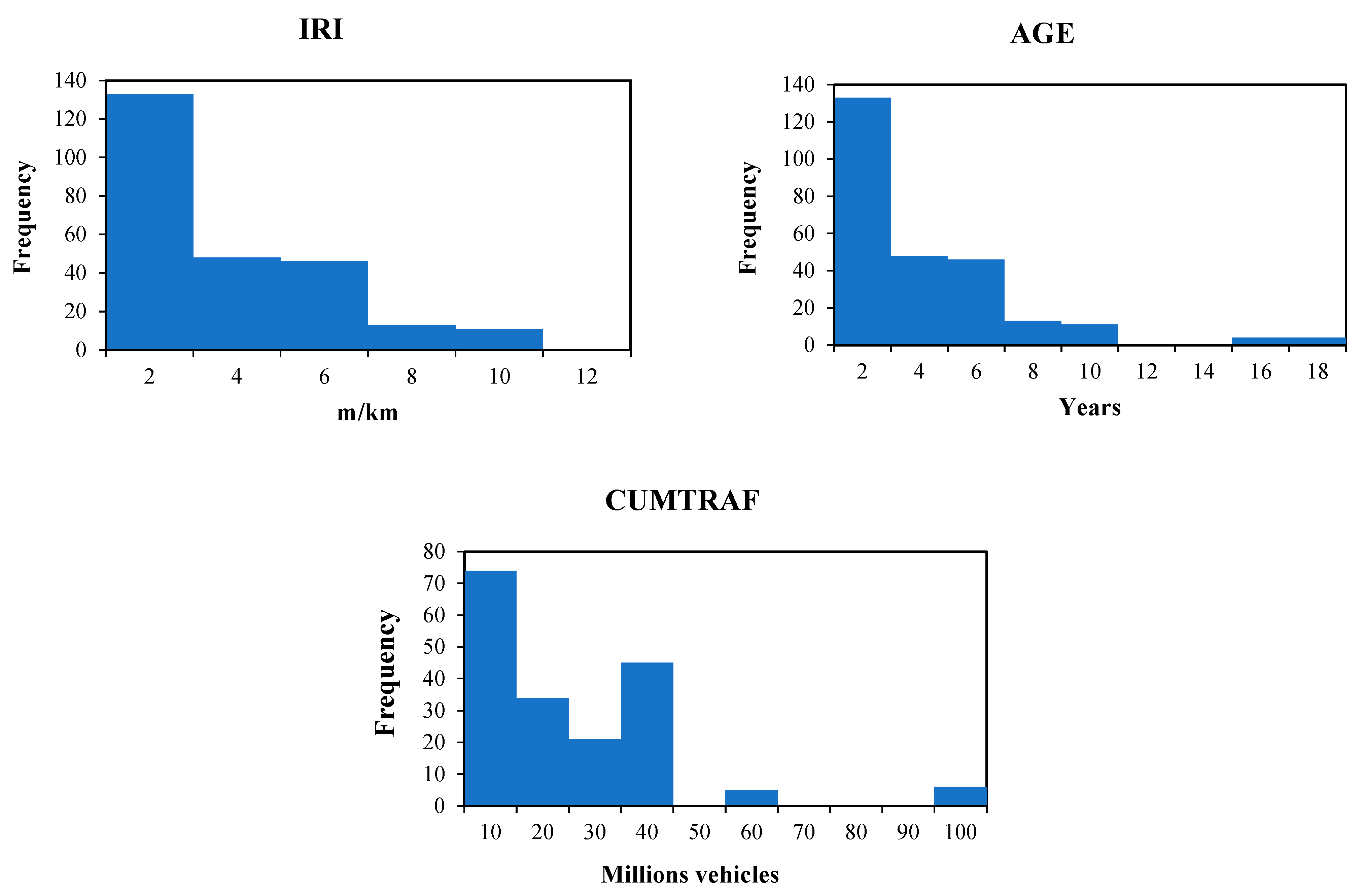
Figure 1. Histogram of the variables.
Sustainability 15 09617 g001
Figure 2. Validation of linear regression model with training and testing datasets.
Sustainability 15 09617 g002
Figure 3. Actual and predicted values of IRI for 20 testing data points.
Sustainability 15 09617 g003
Figure 4. Model validation of machine learning models on testing dataset.
Sustainability 15 09617 g004aSustainability 15 09617 g004b
Figure 5. Global explanation obtained from SHAP analysis for RF model.
Sustainability 15 09617 g005
Figure 6. Average feature importance in RF model based on SHAP analysis.
Sustainability 15 09617 g006
Table 1. Summary of IRI prediction models.
ReferenceFactors UsedIRI Prediction Model
Pérez-Acebo et al. [22]Age, Total thickness of Bituminous layers (TotBit), Accumulated Total number of Heavy Vehicles (TotH.Veh)IRI = 5.353 + 0.68 × e (0.026.R.Age) − 1.411 LnTotBit + 7.941 × 10⁻⁸ TotH.Veh2
Ali et al. [24]Age, Distress (X1,…, X7)IRI = 0.365Age + a1 × 1 + b1 × 2 + … + a7 × 7
Sigdel and Pradhananga [25]Commercial Vehicles (CV), Rainfall (RF), Accumulated low-temperature days (TDl), Accumulated high-temperature days (TDh), Initial IRI (IRI0)IRI = β0 + β1IRI0 + β2CV + β3RF + β4TDl + β5TDh
Qian et al. [26]Equivalent Single Axle Loads (ESAL), Deflection, Overlay Thickness, ClimateSeveral models developed based on different level of each factor
Soncim et al. [27]Traffic Density, ClimateProbability Matrix: Pij(t) = ∑k = 0, mPik(v). Pjk(t-v)
Albuquerque and
Núñez [28]
Modified Structural Number (S), ESAL (N),
Climate (C)
IRI(HMA) = −173.4 + e (5.177 + 0.001C − 0.002S + 0.005N)
Pérez-Acebo et al. [29]Age (R.Age), Accumulated Vehicles (TotVeh), Total thickness of Bituminous layers (TotBit), Accumulated Total number of Heavy Vehicles (TotH.Veh), Coefficient that considers the combinations of materials (BASE), Thickness of the treated base layer (Bthick)IRI = 2.223 + 0.221LnR.Age − 1.162 × 10⁻⁶ TotVeh TotBit + 1.87 × 10⁻⁴ TotH.Veh + BASE Bthick
Table 2. Several studies that engaged machine learning in IRI prediction in pavement performance analysis.
ReferenceData SourcePredictor VariablesMachine Learning ModelR2
(Testing)
AgeTrafficOther
Gong et al. [10]LTPPRF0.95
Ali et al. [30]--RF0.99
SVM0.97
Luo et al. [34]LTPP-XGBoost0.93
SVM0.16
Wang et al. [35]LTPP-RF0.84
DT0.53
SVM0.41
Guo et al. [36]LTPPRF0.88
XGBoost0.90
Damirchilo et al. [37]LTPPRF0.66
SVM0.44
XGBoost0.70
Bajic et al. [38]Denmark--RF0.58
KNN0.59
SVM0.63
Marcelino et al. [39]LTPP-RF0.93
Kargah-Ostadi and Stoffels [40]LTPP-SVM0.90
Ziari et al. [41]LTPPSVM0.83
DT—Decision Tree, XGBoost—Extreme Gradient Boosting.
Table 3. Descriptive statistics of variables used in the study.
Variable Description Mean Standard Deviation Minimum Maximum
IRIAverage IRI value in a road per direction (m/km)2.591.371.519.09
AGETime since the latest rehabilitation/reconstruction activity (years) e.g., 0.5 refers to half of a year (six months).2.753.370.516.5
CUMTRAFCumulative number of vehicles that travelled on the road segment since latest rehabilitation/reconstruction activity (number of vehicles in millions)20.0418.891.2897.95
Table 4. Correlations between IRI and independent variables.
Independent VariableCorrelation with IRISignificance (p-Value)
AGE0.83<0.001
CUMTRAF0.58<0.001
Table 5. Equations describing relationship between each independent variable and IRI.
Independent VariableType of EquationModel AccuracyParameter Estimates
R2F ValueSignificanceInterceptCoefficient b1Coefficient b2Coefficient b3
AGECubic0.76193.92<0.0012.525−0.5060.147−0.006
AGEQuadratic0.69205.17<0.0011.8560.2060.009-
AGELinear0.67392.78<0.0011.6680.336--
AGEExponential0.63309.89<0.0011.8900.085--
AGELogistic0.63309.89<0.0010.5290.919--
AGELogarithm0.42134.46<0.0012.0381.001--
CUMTRAFCubic0.4447.34<0.0011.6620.103−0.003<0.001
CUMTRAFQuadratic0.4162.37<0.0012.234−0.0020.001-
CUMTRAFLinear0.3492.75<0.0011.7520.042--
CUMTRAFExponential0.2974.38<0.0011.9450.010--
CUMTRAFLogistic0.2974.38<0.0010.5140.990--
CUMTRAFLogarithm0.1635.53<0.0011.0850.582--
Table 6. Statistical summary of the multiple linear regression model.
ParameterCoefficientStandard Errorp-Value95% CI
Intercept1.5690.083<0.001[1.410, 1.733]
Pavement age0.3050.021<0.001[0.263, 0.346]
Cumulative traffic0.0100.0030.013[0.002, 0.017]
Table 7. Analyzed multiple regression models with variable transformations for IRI performance.
Proposed ModelR2Standard ErrorF ValueComments
IRI = Intercept + AGE + CUMTRAF20.750.69271.83All variables significant (p < 0.001)
IRI = Intercept + AGE + CUMTRAF + CUMTRAF20.830.57294.80All variables significant (p < 0.001)
IRI = Intercept + AGE + AGE2 + CUMTRAF0.760.69186.64All variables significant (p < 0.006)
IRI = Intercept + AGE2 + CUMTRAF20.810.60400.34All variables significant (p < 0.001)
IRI = Intercept + AGE + AGE2 + CUMTRAF20.820.58284.68All variables significant (p < 0.002)
IRI = Intercept + AGE + AGE2 + CUMTRAF + CUMTRAF20.840.55243.19Low significance of AGE (p = 0.379)
Table 8. Comparison of model accuracy of different machine learning models.
Machine Learning ModelR2MAE
Random Forest (RF)0.9060.310
Decision Tree (DT)0.8700.309
Extreme Gradient Boosting (XGB)0.8090.309
K-Nearest Neighbor (KNN)0.7870.385
Support Vector Machine (SVM)0.5030.579
Disclaimer/Publisher’s Note: The statements, opinions and data contained in all publications are solely those of the individual author(s) and contributor(s) and not of MDPI and/or the editor(s). MDPI and/or the editor(s) disclaim responsibility for any injury to people or property resulting from any ideas, methods, instructions or products referred to in the content.